One Dimensional Chain with Long Range Hopping

Abstract

The one-dimensional (1D) tight binding model with random nearest neighbor hopping is known to have a singularity of the density of states and of the localization length at the band center. We study numerically the effects of random long range (power-law) hopping with an ensemble averaged magnitude $\left\langle|t_{ij}|\right\rangle\propto|i-j|^{-\sigma}$ in the 1D chain, while maintaining the particle-hole symmetry present in the nearest neighbor model. We find, in agreement with results of position space renormalization group techniques applied to the random XY spin chain with power-law interactions, that there is a change of behavior when the power-law exponent $\sigma$ becomes smaller than 2.

I Introduction

The one-dimensional (1D) tight-binding model of non-interacting electrons with random nearest neighbor hopping has been extensively studied since Dyson’s exact solution to density of states of one-dimensional random harmonic oscillators dyson , which can be mapped to the random nearest neighbor hopping model. Mertsching gave a node counting scheme to study the density of states in a similar modelmertsching . Since the early 80s, supersymmetry methods have been used to study such problems with randomnessefetov ; pafisher . All these studies show that there is a singularity in the one-electron density of states $\rho(\epsilon)$ at the band center of the form $\rho(\epsilon)\sim{1\over\epsilon|\ln\epsilon|^{3}}$. Concurrently, as a consequence of the Thouless theorem thouless , there is a logarithmic divergence of the localization length $\xi\sim|ln\epsilon|$. Thus, this model exhibits a critical point at the band center, unlike the standard Anderson modelanderson in one-dimension with on-site disorder, where all states are known to be localizedmott for any finite disorder. This is a consequence of the particle-hole symmetry that is maintained in the model despite randomness in the hopping when only nearest neighbor hopping is present.

In this paper, we investigate in whether these features change if the nearest neighbor hopping model is generalized to include long range hopping. Since these properties are closely related to the particle-antiparticle symmetry in the Hamiltonian, we constrain the long range hopping to a form which preserves the particle-hole symmetry. (Operationally, this is done by allowing hopping only between sites separated by an odd number of lattice constants.) However, the long range hopping terms render analytic methods such as node counting theorom mertsching and Thouless theoremthouless inapplicable; consequently we perform numerical calculations to study this problem instead.

The nearest neighbor tight binding model of non-interacting fermions can be mapped onto a XY spin chain with nearest neighbor random couplings via a Jordan-Wigner transformationlieb . (See, e.g. McKenziermackenzie for a recent discussion of the topic). The singularity in the density of states of the fermion problem at zero energy translates to a singular magnetic susceptibility at zero temperature in the spin problem. Fisherdsfisher , in particular, showed how a perturbative position space renormalization group (RG) scheme using the ratio of small to large couplings for random spin systems employed by several groups in the 80s in the context of random quantum spin-1/2 chainsdasgupta ; bhattlee becomes asymptotically exact, and yields the correct low temperature (energy) behavior. Thus the correct form of the singularity at the band center is obtained for the fermionic model from the asymptotically exact RG. The same position space RG technique has been used recently to study the XY spin chain with long range (power-law) exchange $J(r)\propto r^{-\sigma}$ houck . The behavior found there suggests that the strong disorder fixed point, which determines the functional form of low temperature magnetic susceptibility in the spin problem, (for nearest neighbor hopping this is related to the density of states singularity in the fermionic model) survives for power law exponents $\sigma$ above a critical value, which they determined to be 2 (within their numerical accuracy of 5-10 per cent ).

Using the Jordan Wigner transformation on the 1D XY spin chain with long range couplings, while yielding a particle-hole symmetric fermion Hamiltonian, does not give a pure noninteracting fermion problem with power law hopping [ terms such as $c^{\dagger}_{i}exp(i\pi\sum_{n=i}^{j-1}{c^{\dagger}_{n}c_{n}})c_{j}$ appear as well ]. While the exact connection between the fermionic and spin models is lost when further neighbor hoppings are added to the Hamiltonian, we can nevertheless expect some similarities between the two models - XY random spin chain and free fermions with 1D random hopping - when the two have exchanges/hoppings with a power-law fall off, at least for large power-law exponents. The result for the long range spin model also motivates paying close attention to our model’s behavior when $\sigma$ is in the vicinity of 2.

The outline of our paper is as follows. In the next section, we define the model Hamiltonian. The following section discusses the methods and relevant formalisms used in computation. We then present the results for the density of states, localization length of eigenstates, and the spin-spin correlation function for the equivalent magnetic model, obtained from various numerical calculations. We find that the density of states retains the singularity at the band center, but this singularity is gradually reduced by the long range hopping. The eigenstates are not well described as exponentially localized states, but have power-law-like tails determined by $\sigma$. Finally, the spin-spin correlation function also shows power-law decay where $\sigma$ is not too small.

II The model

The model we have studied is built on a 1D bipartite lattice, consisting of odd and even sites along the chain. The Hamiltonian contains fermionic hopping terms between the two sublattices consisting of the odd and even sites, respectively, while hopping within the same sublattice is forbidden. Thus we have,

$$H=\sum_{<ij>}{t_{ij}(c_{i}^{\dagger}c_{j}+c_{j}^{\dagger}c_{i})}$$ (1)

where $i$ and $j$ are summed over members of the odd and even sublattices respectively. This bipartite property preserves the particle-antiparticle symmetry and leads to interesting properties in the density of states and localization length. The hopping parameters $t_{ij}$ are random with zero average, defined in terms of the distance $|i-j|$ and a Gaussian random variable, as described below. Two models with power law fall-off of $\left\langle|t_{ij}|\right\rangle$ have been studied. Model A allows hopping between every pair formed by picking one site from each of the two sublattices, while $<|t_{ij}|>$ decreases with distance as a power law for each pair $(i,j)$. Specifically, we take

$$t_{ij}={w_{ij}\over\left|i-j\right|^{\sigma}}$$

Where $w_{ij}$ is a Gaussian random number with distribution

$$P(w_{ij})={1\over a\sqrt{2\pi}}\exp\left(-{w^{2}_{ij}\over 2a^{2}}\right)$$

In model B, $<|t_{ij}|>$ is constant, but the probability for a hopping term to be present decreases with the hopping distance as a power-law. Thus

$$t_{ij}=w_{ij}M(\left|i-j\right|)$$

where $w_{ij}$ is a Gaussian random variable as in Model A, and $M(\left|i-j\right|)$ is chosen randomly to be either 1 (with probability $\left|i-j\right|^{-\sigma}$) or 0 [with probability $(1-\left|i-j\right|^{-\sigma}$)].

We expect these two models to exhibit some similarities. We have used a = 0.2 throughout this paper. In both models, therefore, we have only one parameter $\sigma$ which characterizes the model. A small value of $\sigma$ produces longer range hopping.

III Computational Details

The Hamiltonian of this model is an $N\times N$ matrix for a system of N sites, with elements $t_{ij}=0$ when $|i-j|$ is a multiple of 2. Because of this bipartite property, the Schrödinger equation can be written as two coupled equations when number of sites $N$ is even. Let $\psi^{odd}_{i}$ be the wavefunction on the sublattice consisting of the odd numbered sites, and $\psi^{even}_{i}$ that on the sublattice consisting of even sites. If the matrix $h$ represents the hopping terms from even sites to odd sites, then $h^{\dagger}$ will consist of the hopping terms from odd sites to even sites. The Schrödinger equation can then be written as two equations:

$$h\psi^{even} = \epsilon\,\psi^{odd}$$ (2)

$$h^{\dagger}\psi^{odd} = \epsilon\,\psi^{even}.$$ (3)

These equations lead to

$$h^{\dagger}h\psi^{even}=\epsilon^{2}\,\psi^{even}$$ (4)

$$hh^{\dagger}\psi^{odd}=\epsilon^{2}\,\psi^{odd}$$ (5)

The above equations reduce the size of the matrix of the $N\times N$ Hamiltonian to $N/2\times N/2$. Further, from the above equations, it is clear that the eigenvalues come in pairs $\pm\epsilon$, and their eigenvectors are related by

$$\psi^{even}_{\epsilon} = \psi^{even}_{-\epsilon}$$ (6)

$$\psi^{odd}_{\epsilon} = -\psi^{odd}_{-\epsilon}$$ (7)

A direct consequence of the above is that the density of states is symmetric for each realization of the disorder. By exploiting the particle-antiparticle symmetry, we gain efficiency in our numerical calculation.

The density of states can be obtained by directly diagonalizing large matrices. In this approach, the difficulty is that we have to use large matrices which do not have significant finite size effects. Since we’re interested in the property of the singularity at the band center, which by particle-hole symmetry, lies at $\epsilon=0$, we need to get enough statistics near the band center. We identify finite size effects by comparing the results of different sizes.

The other approach to calculating the density of states is a recursive method. First, the dense matrix is cut off at a range large enough, so that the remaining part is an acceptable approximation for the original matrix of arbitary size. [ For finite range hopping, this method gives no approximation at this stage, but for long-range (power law hopping) this is a different cutoff scheme, with a somewhat different finite size effect ]. Then the matrix $H-\epsilon$ is transformed into diagonal form by a similarity transformation, which rotates certain columns and rows to eliminate off-diagonal terms. The remaining diagonal elements are not eigenvalues, but they retain the signature of the matrix, i.e., a positive element implies an eigenvalue satisfying $E_{i}>\epsilon$, a negative element corresponds to an eigenvalue satisfying $E_{i}<\epsilon$. By counting the number of positive or negative diagonal elements we can obtain the integrated density of states. This process can be continued for arbitary length with no finite-size effect as in direct diagonalization, until the statistical error of the integrated density of states is smaller than our requirement. For nearest neighbor model, the recursion equation for diagonal element is:

$$\zeta_{n}=-\epsilon-{H_{nn-1}^{2}\over\zeta_{n-1}}$$

where $H_{nn-1}$ is the only off-diagonal term in the Hamiltonian, $\zeta_{n}$ is the remaining diagonal element after the transformation. Suppose $\zeta_{n}$ has a distribution $F(\zeta)$ as $n\longrightarrow\infty$, then it is given by the integral equation

$$F(\zeta)=\int_{-\infty}^{+\infty}\delta(\zeta+\epsilon+{x\over\xi})P(x)F(\xi)dxd\xi$$

where $P(x)$ is the distribution function of $H_{nn-1}^{2}$. Although this equation is similar to Dyson’s approach dyson , it has not been solved analytically due to the peculiar argument of the $\delta$ function. The numerical approach is just to generate a sequence of $\zeta_{n}$ and calculate its distribution.

To take care of the finite size effect introduced by the cut-off, we compare results using different cut offs. Such a procedure allows us to ascertain the range of energies for which the integrated density of states has converged: lower the energy, longer the cut-off required (the cutoff required varies roughly logarithmically with energy). For a fixed cutoff, the energy variation of the integrated density of states obtained by this method mimics that of the nearest neighbor i.e., finite range model - this sets the lower bound of energies close to the band center for which this method is applicable for that cutoff.

Once we have obtained the eigenfunctions by direct diagonalization, we can calculate the correlation function of the corresponding spin model. The Jordan-Wigner transformation lieb transforms the XY-spin chain in zero external field to a half-filled band of fermions, because the following identity

$$\sum_{i}S_{i}^{z}=\sum_{i}c_{i}^{\dagger}c_{i}-{N/2}$$ (8)

The ground state fills the $N/2$ states with negative energy which we can get by diagonalizing the Hamiltonian. We can further calculate the spin correlation function on the ground state. We compute the zz part of the spin-spin correlation function defined by

$$C(i,j)=\overline{\left\langle S^{z}_{i}S^{z}_{j}\right\rangle}$$ (9)

$\left\langle...\right\rangle$ denotes the expectation value in the ground state, while the bar on top denotes ensemble average over the disorder. With $S^{z}_{i}=c^{\dagger}_{i}c_{i}-{1\over 2}$, and $i\neq j$, the correlation function can be written as

$$C(i,j)=\overline{\left\langle c^{\dagger}_{j}c^{\dagger}_{i}c_{i}c_{j}\right\rangle}-{1\over 4}$$ (10)

where we have used the fact $\overline{\left\langle c^{\dagger}_{i}c_{i}\right\rangle}={1\over 2}$ due to half filling. The Jordan-Wigner transformation contains a phase factor due to the anticommutation relation of fermion operators on different sites, but the phase factor coming from different fermion operators cancels each other in our expression of $C(i,j)$. In the random singlet phasepafisher appropriate for describing the nearest neighbor only model in the spin operator language, all these correlation functions have the same dependence on distance. The four fermion term can be expanded into a Hartree term and a Fock term.

$$\left\langle c^{\dagger}_{j}c^{\dagger}_{i}c_{i}c_{j}\right\rangle=\sum_{n,m,occupied}\psi_{n}^{\dagger}(i)\psi_{n}^{\dagger}(i)\psi_{m}(j)\psi_{m}(j)$$

$$-\psi_{n}^{\dagger}(i)\psi_{n}^{\dagger}(j)\psi_{m}(j)\psi_{m}(i))$$

Here the sum is over all occupied states, i.e. all N/2 states with negative energy. The Hartree term can be evaluated directly to be $1/4$ because the wavefunctions are orthonormal using equations (6) and (7). Therefore the correlation function is given by the Fock term only. Further, if $i$ and $j$ are on the same sublattice, we see from equations (4) and (5) that $\psi_{n}(i)$ and $\psi_{n}(j)$ ( n is among $N/2$ occupied states) are both eigenvectors of either $h^{\dagger}h$ or $hh^{\dagger}$, and consequently orthogonal to each other. Thus, when $i$ and $j$ are on the same sublattice, the correlation function is exactly zero. In the numerical results presented below, we only display the spin correlation functions between 2 sublattices, and $C(i,j)$ is replaced by $C(x)$ where $2x+1=|i-j|$.

$$C(x)=-\sum_{m,n,occupied}\overline{\psi_{n}^{\dagger}(i)\psi_{n}^{\dagger}(j)\psi_{m}(j)\psi_{m}(i)}$$ (11)

This expression can be evaluated directly, but since the computing time for evaluating C(x) is even more than that required for diagonalization, the system sizes we use are smaller than for diagonalization. The data presented for C(x) are all obtained from systems of 256 sites. However, we are able to discern the behavior reasonably well from the data for $C(x)$ subject to this limitation.

IV Density of States

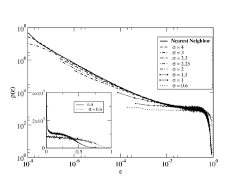
Figure 1: Density of states of model A for different values of the power law exponent $\sigma$, shown on a double logarithmic plot, showing the singularity at the band center ($\epsilon=0$). The inset shows the data on a linear scale. The singularity becomes very weak when $\sigma$ is less than 2, and is not discernable for the sizes studied when $\sigma$ is below 1.

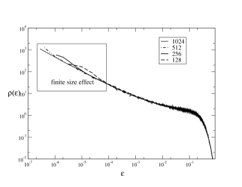
Figure 2: The same data as in figure 1, plotted in a different way as motivated in the text. As expected, the density of states of the nearest neighbor model asymptotically falls on a straight line. The upwards bending of the curves with decreasing $\sigma$, evident for $\sigma<3$ shows the weakening of the density of states singularity by the long range hopping.

Our results on model A show that the density of states remains singular at the band center when the long range hoppings are present. Figure 1 shows the density of states $\rho(\epsilon)$ obtained by diagonalization as a function of energy $\epsilon$ on a double logarithmic plot for both the nearest neighbor model, and for the long range model for different values of the power law exponent $\sigma$. As can be seen, the singularity at the band center ($\epsilon=0$) persists at least for large $\sigma$, though its magnitude clearly decreases. The inset to Fig 1 compares the data for the nearest neighbor model along with the data for the lowest power law ($\sigma=0.6$) on a linear scale, which gives a clearer idea of the extent of this decrease. For quantitative purposes, it is better to plot the same data as $(\rho(\epsilon)\epsilon)^{1/3}$ vs.$\ln\epsilon$. On such a plot, shown in fig 2, the nearest neighbor model is supposed to lie on a straight line, which it clearly does. Further, the curves show little deviation from the nearest neighbor model as long as $\sigma>3$. The deviation for smaller $\sigma$ are consistent with the singularity being gradually weakened as $\sigma$ decreases; if we fit the data with $\rho(\epsilon)\sim{1\over\epsilon|\ln\epsilon|^{\omega}}$ then when $\sigma=2$, the best fit $\omega$ is about 5. As $\sigma$ becomes lower than 1, direct diagonalization is almost incapable of revealing any detail of the singularity: we only see a large value at the band center, and the density of states approaches the Wigner semicirclewigner . Nevertheless, the thermodynamic limit remains well defined upto $\sigma=0.5$, below which the bandwidth starts to increase with system size, i.e. we need to scale the hopping magnitude with system size to have a sensible thermodynamic limit. This critical value of $\sigma$ can be predicted by writing the model in path-integral form, using either replica technique or supersymmetry, and averaging over the random variables. Such an approach gives a four fermion term proportional to $\Sigma|i-j|^{-2\sigma}$, where $i$ and $j$ are site indices, therefore when $\sigma$ is less than 0.5, the sum will diverge.

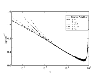
Figure 3: Finite size effects on density of states, which appear at the low energy end of these curves. Data are density of states for four different size systems with the same $\sigma=2.5$, with length varying from $N=128$ to $1024$.

We have diagonalized several different sizes of samples to ensure that the data shown are not corrupted by finite size effects. Fig. 3 shows an example of a finite size effect, which appears as a size-dependent rounding of density of states at low energy. All the data plotted correspond to N = 1024 sites unless stated otherwise, and do not suffer significant finite size effects. The results of model B are very similar to model A, except that the smallest $\sigma$ for a proper thermodynamic limit to exist is 1.

Fig 4 shows our results for the density of states obtained using the recursive method. Here, one obtains the integrated density of states $N(\epsilon)$ (from $0$ to $\epsilon$). For the nearest neighbor model, the exact asymptotic form is given by:

$$N(\epsilon)\sim{1\over|\ln\epsilon|^{2}}$$

Fig 4 plots the inverse square root of $N(\epsilon)$ versus $\ln\epsilon$; for the nearest neighbor model, the expected straight line behavior is seen. For power law hopping, the data shows measurable curvature certainly for $\sigma=2.5$. For larger $\sigma$ it is difficult to see whether the data suggest curvature, or simply a changing slope with decreasing $\sigma$. While it is tempting to fit these curves with a form like

$$N(\epsilon)\sim|\ln\epsilon|^{-\lambda}$$

, which will lead to an singularity in the density of states like $\rho(\epsilon)\sim 1/(\epsilon|\ln\epsilon|^{\lambda+1})$, the data are better fit with several $\lambda$. This suggests that corrections to the asymptotic form may be important for power law hopping.

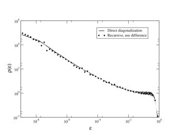
Figure 5: Comparison between the recursive method and the direct diagonalization method for the density of states. The solid curve is by direct diagonalization, while the points are density of states obtained by taking the difference of integrated density of states from the recursive method. The agreement between the curves is good, and no systematic errors are found.

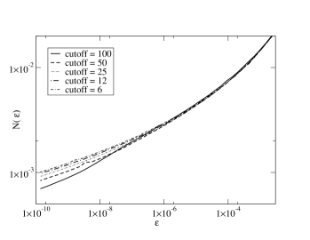
Figure 6: Convergence of the recursive method exhibited using different cutoff parameters for the hopping. Small values of the cutoff lead to deviations starting from higher energies.

In figures 5,6, we show the accuracy of this recursive method. Figure 5 shows a direct comparison of the two methods.The recursive method agrees with the diagonalization results before the finite size effect sets in. Figure 6 shows the convergence of the recursive method as the range of cut-off is increased. (Below a certain energy, which corresponds to distances beyond the cutoff length, the recursive method will behave like nearest model, since the wavefunction spreads out of the range of hopping).

The density of states allows us calculate the specific heat and spin susceptibility for this this model of non-interacting fermions. Using the standard formulaesmith , we can see that the specific heat prefactor ($\gamma$, where $c_{v}=\gamma T$) and susceptibility ($\chi$) at low temperature are singular at the center of the band. Thus, in the vicinity of the band center the zero temperature susceptibility is the form:

$$\chi\sim{1\over T|\ln T|^{\omega-1}}$$

if the singularity in density of states is $1\over\epsilon|\ln\epsilon|^{\omega}$. A similar formula holds for $\gamma$.

V Localization Length

The nearest neighbor model is known to have a sigularity in the localization length ($\xi$) at center of the band. It’s asymptotic form is

$$\xi\sim|\ln\,\epsilon|$$ (12)

This singularity can be deduced from the singularity of density of states using the Thouless theoremthouless . However, in the longe range hopping model, the theorem does not apply, and our numerical calculation suggests that the behavior of the two models is rather different.

For finite energy, all states are found to decay from a central maximum in both models, and the decay becomes weaker as the band center is approached, as in the nearest neighbor model. However, the behavior with distance is rather different for the two models.

• In the case of model A which has genuine long range (power law) behavior of the hopping parameter $t_{ij}$, the tail of the wavefunctions actually decay in a power-law manner, $\psi(x)\sim x^{-\sigma}$. This form is obviously determined by the power-law long range hopping term. If we apply the usual method of looking at the asymptotic behavior to determine localization length, the localization length is infinite for any power law exponent!

• In the case of model B, the wavefunction is found to be decaying exponentially at long distances, like the nearest neighbor model, and the localization length can be obtained by several methods, which agree with the theoretical prediction.

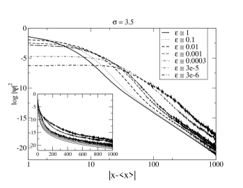
Figure 7: Double logarithmic plot of the probability density in real space for individual eigenstates plotted from the center of each state, averaged over eigenstates with a given energy $\epsilon$ for model A with $\sigma=3.5$. Small values of $\epsilon$ correspond to states near the band center. We can see as the energy approches the band center, the states become more delocalized. In the tail, for all energies, the profile of the wavefunction actually decreases in a power-law fashion, with an exponent exactly determined by the value of $\sigma$. Similar plots for other values of $\sigma$ in model A show the same feature. The inset with the probability density on a semilog plot, shows distinct curvature in the tail, unlike an exponentially localized state.

Fig 7 shows a log-log plot of the averaged probability density (wavefunction amplitude squared $|\psi|^{2}$) as a function of the distance from the center of the wavefunction, averaged over typically 512 states, as a function of energy away from the band center for model A. At long distances, the behavior is clearly linear on this double logarithmic plot, implying a power law decay at long distances. Fitting the data shows clearly that the decay is related to the power law behavior of $t_{ij}$ - the tail of $|\psi|^{2}$ decays as $1\over|x-<x>|^{-2\sigma}$. This tells us that we cannot use the localization length, as defined by Thouless for an exponentially decaying state here. However, we may usefully define moments of the wavefunction to compute, for example, inverse participation ratiosipr .

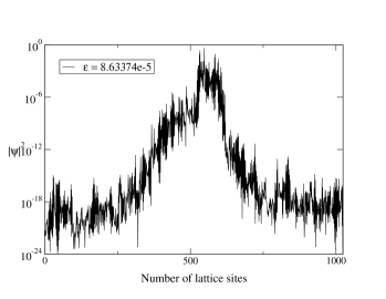
Figure 8: A typical wavefunction of model A near the band center(small $\epsilon$) shown on a log-linear plot

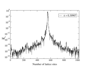
Figure 9: A typical wavefunction of model A away from the band center(larger $\epsilon$) on a log-linear plot. The tail shows clear curvature on this plot, implying a functional form that decays slower than exponential.

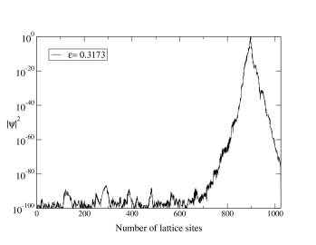
Figure 10: A typical wavefunction of model B away from the band center. A clear exponential decay of the wavefunction amplitude over 50 decades is seen, as in the nearest neighbor model.

The problem of defining the localization length in model A is not shared by model B, where we find that the wavefunctions always decay exponentially. To show this difference, in Figures 8 to 11 we have plotted typical wavefunctions for model A and model B (on a log-linear plot of probability density versus distance) near the center and in the tail of the band. The difference between the two models near the center of the band is not obvious due to the large fluctuations, but in the tail of band, they look clearly different - model B shows straight exponential decay (see Fig. 10) down to 50 orders of magnitude for $|\psi|$, while model A (see Fig. 9 ) shows clear upwards concave curvature in the tail, characteristic of a slower decaying function (like a power law) at long distances.

VI Spin Correlation Function

We now present results for the spin-spin correlation function for the associated model in terms of the spin operators obtained by a Jordan Wigner transformation. The motivation is to compare the results with those obtained for the long range random antiferromagnetic XY spin chainhouck . We reiterate that because of long range hopping, our model contains terms in addition to those in the pure power law XY model studied by Houck and Bhatt; however, because of the existance of the same long range two-spin interactions in both studies, there may be several points in common.

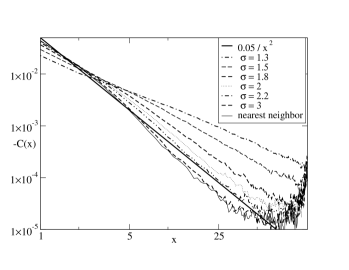
Figure 12: Spin-spin correlation function in the ground state ($T=0$), for the corresponding spin model obtained using a Jordan-Wigner transformation. The bold straight line, which decays as $1\over x^{2}$, is a guide for the eye. We see that when $\sigma$ is above 2, including nearest neighbor model, $C(x)$ exhibits this inverse square behavior. Below $\sigma=2$, $C(x)$ is better fitted by $1\over x^{\sigma}$. More sample averaging is necessary to smooth the noisy tail at long distances.

Figure 12 shows the average correlation function $C(x)$ obtained by averaging 256 samples of model A each having 256 sites plotted on a double logarithmic plot. All the values of $C(x)$ are negative (corresponding to antiferromagnetic correlations). Our results suggest that there are three regions of distinct behavior, which can be summarized as given below:

• For fast power law decays (i.e., exponents $\sigma>2$ ), the long distance behavior of the correlation function remains unchanged from the nearest neighbor model. Thus in Figure 12, the curves are parallel to each other at large $x$ values, consistent with the result for the nearest neighbor model, for which a slope of 2 is predicteddsfisher . (For example, a best fit of $C(x)$ for x within the interval $[20,60]$ $\sigma=2.2$ yields a slope of 1.97).

• When $\sigma$ gets below 2, the slope begins to change. For $\sigma$ close to but less than 2, the slope appears to be given by $\sigma$ itself, implying $C(x)\sim x^{-\sigma}$. ( A least squares fit to $C(x)$ of the form $C(x)={a\over x^{v}}$, gives $v=1.79$ for $\sigma=1.8$, $v=1.44$ for $\sigma=1.5$ and $v=1.12$ for $\sigma=1.3$). Our numerically exact results thus show that the model’s magnetic counterpart changes its low energy behavior different behavior for power law exponents $\sigma$ below 2. This is precisely the value around which Houck and Bhatthouck found that the perturbative real-space RG procedure appears to break down, perhaps signalling a change of phase.

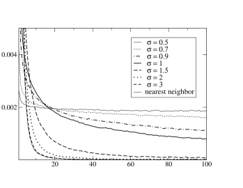
Figure 13: Spin-spin correlation function, as in figure 12, plotted on a linear scale. For $\sigma<1$ $C(x)$ decays very slowly, and seems to approach a constant value at large distances.

• Below $\sigma\sim 1$, the deviations of $C(x)$ from the nearest neighbor model become rather significant. To exhibit this more clearly, we show a linear plot in Figure 13. C(x) seems to decay very slowly, and our data are consistent with it approaching a finite (negative) value, implying antiferromagnetic order. (For example, the curve for $\sigma=0.7$ is well fitted by ${a\over x^{v}}+d$, where $v=0.49$ is 1/2 within numerical accuracy). We caution, however, that for such low power law decays, finite size effects can be large, and more detailed calculations with larger system sizes and more samples is necessary before this result can be stated with certainty from numerical studies.

In summary, the numerical results on the spin correlation function from the long range fermion model (which we can solve numerically exactly) supports the earlier observations on the XY chain with random long range couplings using perturbative numerical RG methods that the random singlet phase is unstable for power law couplings with exponents less than 2. However, unlike the numerical RG study, which sees this as a breakdown of the RG scheme, we are able to go into the new phase, which appears to be characterized by continuously varying exponents, like a critical phase. We also find evidence for a possible transition to long range order at still smaller $\sigma$. It should, however, be borne in mind that these observations, are from numerical calculations in finite systems, and subject to statistical errors due to finite sampling of the quenched random variable.

VII Summary

In this paper, we have presented results of a numerical study of a one dimensional lattice model of non-interacting fermions with random long range (power-law) hopping, which maintains particle-hole symmetry of the nearest neighbor model by allowing hopping only between even and odd sites (i.e., no hopping allowed between odd sites, or between even sites). We have studied two models - one with genuine power-law hopping, and another with long range hopping with a power law fall-off of the probability of such a hopping to be present. The results on density of states, localization and spin correlation function of the two models have been presented and analysed.

For the density of states, we observe that the singularity at the center of the band, present for the nearest neighbor model, is weakened by long range hopping (Model A). The change is gradual, and at least for power-law exponents $\sigma$ greater than 3, is consistent with a change in the prefactor of the singularity. For $\sigma$ less than 3, though, the numerical data for the desity of states in the range available appear to fit better with a somewhat different power of the logarithm of the energy. Beyond $\sigma=1$, the data are consistent with no singularity being present, until $\sigma<0.5$, when the thermodynamic limit becomes ill-defined. Similar results are seen in Model B, except that the thermodynamic limit becomes ill-defined at $\sigma=1$.

The two models exhibit rather different behavior of the electronic wavefunctions. Model B is conventional, in that its wavefunctions are exponentially localized, just as the eigenstates of nearest neighbor model. In model A, however, the wavefunctions are actually localized in a power-law manner rather than exponential. Consequently, the usual definition of localization length in terms of the logarithm of the long distance behavior of the wavefunction is invalid; however, several inverse participation ratios can still be defined.

By transforming the fermion model back to a spin model using Jordan-Wigner transformation, we calculated the spin correlation function in the ground state. Based on the data, three different phases may be possible - (1) the random singlet phase, which seems to be stable for power law exponents down to $\sigma=2$; (2) a critical type phase with a continuously varying exponent of the power-law characterizing the spin-spin correlation function between $\sigma=2$ and $\sigma=1$; and (3) a possibly long-range ordered phase for $\sigma<1$.

VIII Acknowledgement

This research was supported by NSF DMR-9809483.

Figure 4: Integrated density of states, computed by the recursive method, with cut-off at 100th neighbor. Within the displayed energy range, these curves are checked to be free of effects due to the finite cut-off in the hopping range. Note that the curves are smoother than the results obtained from straight diagonalization. The nearest neighbor model is expected to asymptotically fall on a straight line with a slope equal to -1. Curves fitted by the formula $N(\epsilon)\sim{1/|\ln\epsilon|^{v}}$, yield $v$ somewhat larger than the value 2 appropriate for the nearest neighbor model, for $\sigma$ below 3.

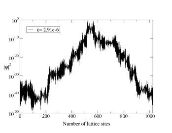
Figure 11: A typical wavefunction of model B near the band center. Despite strong fluctuations, the main profile is basically exponential, as in the nearest neighbor model.

References

- (1) F. Dyson, Phys. Rev. 92,No. 6 1331-1338(1953).
- (2) J. Mertsching, Phys. stat. sol(b) 174, 129 (1992).
- (3) T. Bohr and K. B. Efetov J. Phys. C 15, L249(1982).
- (4) Leon Balents and Mathew P. A. Fisher, Phys. Rev. B 56 12970 (1997).
- (5) P. A. Anderson Physical Review 109, 1492 (1958).
- (6) N. F. Mott and W. D. Twose, Adv. Phys.10, 107 (1961); R. E. Borland, Proc. Royal Soc. A 274, 529 (1963).
- (7) R. H. McKenzie, Phys. Rev. Lett. 77, 4804 (1996).
- (8) C. Dasgupta and S. -k. Ma Phys. Rev. B 22, 1305 (1980).
- (9) R. N. Bhatt and P. A. Lee, Jour. Appl. Phys. 52, 1703 (1981).
- (10) See e.g. M. L. Mehta, Random Matrices, ( Academic Press, Boston, 1991 ).
- (11) D. J. Thouless J.Phys.C, 5, 77-81 (1972).
- (12) A. A. Houck, Junior Independent Project (Princeton University, 1999); A. A. Houck and R. N. Bhatt (unpublished).
- (13) E. Lieb, T. Schultz, and D. Mattis, Annals of Physics 16,407-466 (1961).
- (14) E. R. Smith, J. Phys. C, 3,1419-1432 (1970).
- (15) D. S. Fisher Phys. Rev. B 50 No.6 3799-3821,(1994).
- (16) For example, the nth inverse participation ratio may be defined by where is the normalized wavefunction.