Quantum discrete $\phi^{4}$ model at finite temperatures:
the mean-field phase diagram

Abstract

The quantum discrete $\phi^{4}$ model at finite temperature is studied in the mean-field approximation. The phase diagrams are obtained for a wide range of the model parameters. The domains of applicability for the classical, quantum, and order-disorder limits are determined. It is shown that a remarkable part of the phase diagram is reproduced by the first quantum correction to the classical result. Parameters of Sn₂P₂S₆, SrTiO₃, and KH₂PO₄ are placed in the phase diagram of the model.

Physics Department, Moscow State University, 119899 Moscow, Russia

1 Introduction

Quantum zero-point fluctuations play an important role in the ferroelectric phenomena for a wide range of ferroelectric materials [1]. Some of the materials, such as SrTiO₃, show a displacive (soft-mode) phase transition, while others are of the order-disorder type, for example the hydrogen-bond KH₂PO₄. Therefore, from the fundamental point of view, one should answer the two questions to characterize each material: (i) what is the interplay of quantum (zero-point) and classical (thermal) fluctuations and (ii) how close the transition is to the order-disorder or displacive scenarios. Working with model Hamiltonians, it is suitable to consider the quantum discrete $\phi^{4}$ model here. The variation of the model parameters allows to go continuously from the displacive to the order-disorder second-order transition. An introduction of a finite mass and Plank constant gives rise to the zero-point fluctuations in the model.

Although the discrete $\phi^{4}$ lattice is one of the simplest possible microscopic models for the phase-transition phenomena, the studies have been restricted to the asymptotical cases so far. In the general case the transition type is neither purely displacive nor order-disorder and (or) fluctuations are neither purely quantum nor thermal. Up to our knowledge, there is no a quantitative investigation of this situation so far. Moreover the exact values of the model parameters are not clear, than the known asymptotical cases realize. This paper is aimed, in particular, to solve the latter problem.

Let us write down the explicit formulae and discuss the known asymptotical behaviour. The discrete $\phi^{4}$ model is a cubic lattice of 2-4 anharmonic oscillators, with a nearest-neighbour harmonic coupling. The Hamiltonian can be written as follows [2]:

$$H = \sum_{n}\frac{P_{n}^{2}}{2M}+V,$$ (1)

$$V = -\frac{A}{2}\sum_{n}x_{n}^{2}+\frac{B}{4}\sum_{n}x_{n}^{4}+\frac{C}{2}\sum_{nn^{\prime}}(x_{n}-x_{n^{\prime}})^{2}\sigma_{nn^{\prime}}.$$

Here $x_{n}$ is the displacement of the $n$-th atom in the unit cell, $A,B,C$ are parameters of the model. The first two terms in the potential energy $V$ form a double-well potential and the last term stands for the interaction. There is only the inteaction between nearest-neighbours in the model, i.e. $\sigma_{nn^{\prime}}=1$ if $n,n^{\prime}$ are the nearest neighbours and vanishes elsewhere. Note that the Hamiltonian (1) includes the displacement of atoms, but not the actual distance between them.

If there were no any fluctuations in the system, all atoms would occupy the same position in the cell $x_{n}=\sqrt{A/B}$ (or $x_{n}=-\sqrt{A/B}$). There are two sources of fluctuations. The dimensionless mass $m=MCA^{2}/\hbar^{2}B^{2}$ determines the role of quantum zero-point fluctuations in the model (the system is classical at $m\to\infty$). The classical thermal fluctuations are governed by the reduced temperature $t=TB/AC$ (the system becomes purely quantum at $t=0$). Large fluctuations can destroy the ordering, so that the average of $x$ vanishes. The system of a dimensionality $d>1$ shows a second-order transition for any positive $A,B,C$. The parameter $a=A/C$ determines the type of the transition: displacive transition corresponds to $a\to 0$, while the limit $a\to+\infty$ corresponds to the order-disorder system [3, 4]. At a given $a$ there is a critical line $t_{c}(m_{c})$ in the $t-m$ phase diagram (hereafter the subscript ”c” stands for the critical values of temperature and mass).

In the reduced dimensionless variables, the Hamiltonian takes the form

$$h=-\sum_{n}\frac{\nabla_{n}^{2}}{2m}+v,$$ (2)

$$v=\left(2d-\frac{a}{2}\right)\sum\limits_{n}{x_{n}^{2}}+{a\over 4}\sum\limits_{n}{x_{n}^{4}}-\sum\limits_{n,n^{\prime}}{x_{n}x_{n^{\prime}}}\sigma_{nn^{\prime}}.$$

The asymptotical cases are studied extensively. Basically, they are the follows.

At the limit $a\to+0$ the transition is of the soft-mode type. This asymptotic is studied at $t=0$, as well as at finite temperature [5, 6]. Since the double-well potential is small for this case, it can be treated as a perturbation. Therefore a convenient method of the investigation of this limit is the independent-mode approach [2]. The system is harmonic in the zero approximation, therefore the phonon vibrations $Y_{k}\propto\sum e^{ikj}x_{j}$ can be treated as uncoupled oscillators so that one assumes $<Y_{k}Y_{l}>\propto\delta(k+l)$ (hereafter the triangle brackets stand for the averaging over thermal and quantum fluctuations). In the first approximation the anharmonic term renormalize the phonon dispersion. Virtually, the real interaction can be reduced to an effective (i.e. dependent on the temperature and mass) harmonic one. At certain values of $t$ and $m$ the zero-frequency mode (soft-mode) appears in the system indicating the phase transition. The independent-mode approach is exact in the $a\to+0$ limit. However, serious difficulties appear for a finite $a$; particularly, $t_{c}$ and $m_{c}$ are incorrectly predicted to be independent on $a$ in the independent-mode scheme.

At the opposite limit $a\to+\infty$, the discrete $\phi^{4}$ model shows an order-disorder phase transition. The physical picture in this case is the follows. Since an on-site potential is much larger than all other energy scales, atoms are localized in either left or in the right side of the double-well in the zero approximation: $x_{n}\approx\pm\sqrt{A/B}$. Therefore, each oscillator can be treated as a two-level system. The tunnel coupling between the two sides of a well produces some energy splitting $\Gamma$, which depends on the mass $m$ implicitly. This case coincides with the transverse-field Ising model [7, 8]. This model describes an array of $\frac{1}{2}$-spin particles in the external field with a nearest-neighbour interaction between particles. The Hamiltonian of this model is

$$H=-\Gamma\sum_{i}S_{i}^{x}-\frac{C}{2}\sum_{i,j}\sigma_{nn^{\prime}}S_{i}^{z}S_{j}^{z},$$ (3)

where $S_{i}^{x}$, $S_{i}^{z}$ are $\frac{1}{2}$ spin operators. The phase transition can be observed by changing the two parameters: temperature $t$ and transverse field $\Gamma$. The transverse-field Ising model is also widely studied at $t=0$ and at finite temperature by various approximations. High-temperature series expansions, ground-state perturbation theory, correlated-basis-function analysis, random phase approximation and its generalizations, $1/\Re$ and $1/S$ expansions, continuum field theory methods have been used [7, 8, 9, 10, 11, 12, 13].

The classical case corresponds to the condition $m\to\infty$. In this case the momentum-coordinate uncertainty is small, so that the partition function can be factorised as $Z=\int\exp(-\sum\limits_{n}p_{n}^{2}/2mt)d^{N}p_{n}\cdot\int\exp(-v/t)d^{N}x$. The temperature dependence of the order parameter is determined here by the second term and is therefore independent of mass $m$. The dependence $t_{c}(a)$ is studied both numerically and by analytical approaches for 2D, layered and 3D systems [3, 4]. An extension of the mean-field scheme has been developed, which is appropriate for the description of Monte Carlo results with a good accuracy in a wide rage of parameter $a$.

The quantum limit takes place at $t=0$ and at finite mass $m$. The dependence $m_{c}(a)$ is studied [14] by quantum Monte Carlo simulations and the simplest analytics for a wide range of $a$.

In this paper, we study the phase diagram of the quantum discrete $\phi^{4}$ model for a full range of parameters, and determine the domain of applicability for the asymptotical results mentioned above. We also consider the leading-order quantum correction to the classical result. In a conclusive part of the paper the parameters of several ferroelectric materials are placed in the phase diagram obtained.

We chose the mean-field (MF) approximation for the study because of its simplicity. Actually, we are interested in quite crude characteristics such as the domains of applicability. Therefore we believe that this method is suitable here, although it is not very accurate. The validity of the MF approach is discussed in more details in the end of the paper.

2 The quantum mean-field approximation

In the MF approach, the real interaction between particles is replaced with an interaction of the on-site oscillator with an external field $E=4d<x>$. The self-consistent set of MF equations for $<x>$ is formed by this formula and the expression for the average displacement of the on-site oscillator [15]

$$<x>=\frac{{\rm Sp}\left(xe^{-(H_{0}-E<x>)/T}\right)}{{\rm Sp}\left(e^{-(H_{0}-E<x>)/T}\right)},$$ (4)

where

$$H_{0} = \frac{P^{2}}{2M}+V_{0},$$ (5)

$$V_{0} = \left(2dC-\frac{A}{2}\right)x^{2}+\frac{B}{4}x^{4}.$$

In this paper, we are interested in the position of the transition point in phase diagram. The condition $<x>\to 0$ is fulfilled in the point of the phase transition. Keeping the leading-order in $<x>$ terms, one obtains the MF equations for the critical point:

$$4dC\chi_{1}=1,$$ (6)

where $\chi_{1}$ is the static linear susceptibility, which is determined at the finite temperature by the standard quantum-mechanical formula [16]:

$$\chi_{1}=\sum_{ij}\frac{2d_{ij}^{2}}{E_{i}-E_{j}}\exp{\frac{F-E_{i}}{T}}.$$ (7)

Here, $F=-T\ln Z$ is the free energy ($Z$ is a partition function), $E_{i}=<i|H_{0}|i>$ and $d_{ij}=<i|d|j>$ are respectively the eigenenergies and the dipole matrix elements for the on-site Hamiltonian $H_{0}$, defined in Eq. (5).

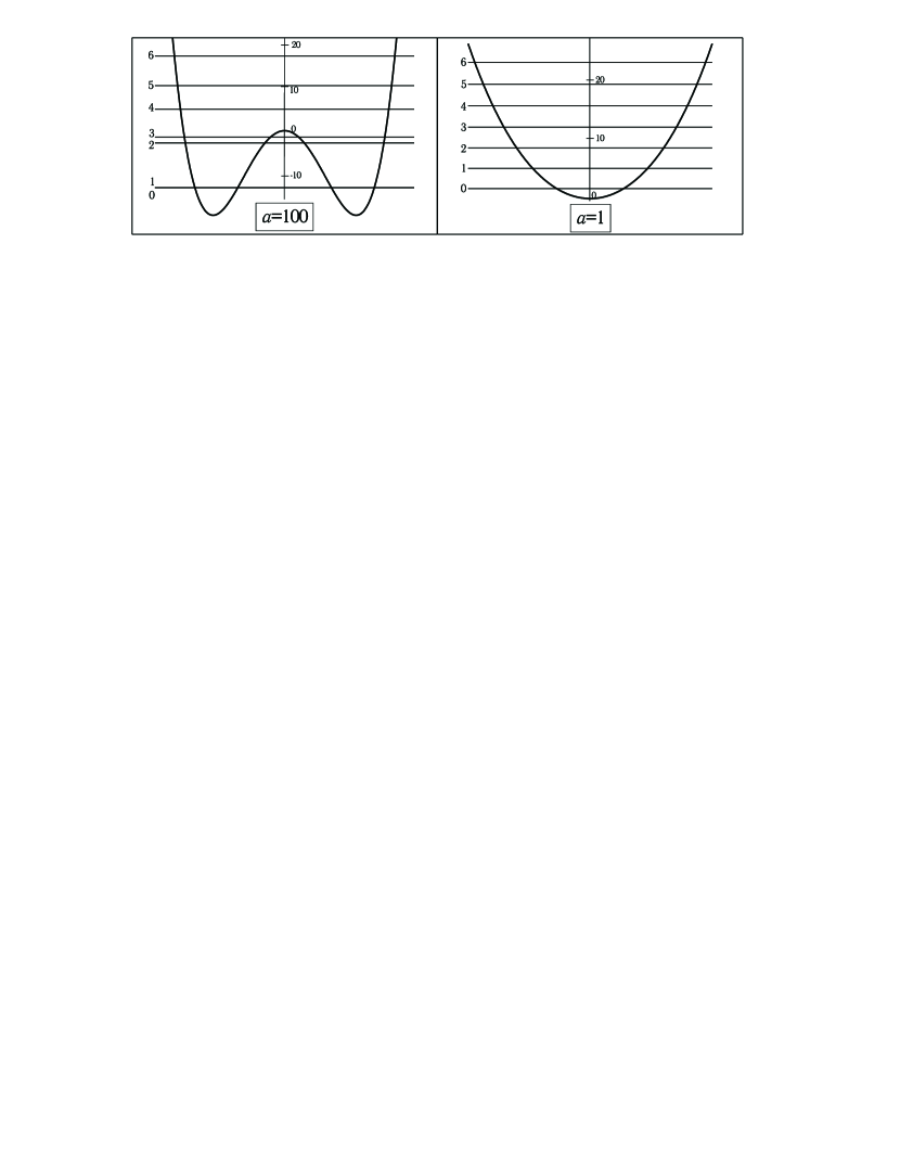
Figure 1: The on-site potential and its spectrum for the two limits of the discrete $\phi^{4}$ model. The left panel is a typical spectrum for the order-disorder limit ($a=100$). The right panel is a typical spectrum for the displacive limit ($a=1$). Parameters $m=1$ and $d=3$ are used for the both cases.

Let us briefly discuss the structure of the spectrum. In the displacive limit $a\to+0$ it is almost equidistant, because the nonlinearity of the potential is small. In the order-disorder case of $a\to+\infty$ the situation is quite different. There are several doublets of the lowest levels, whereas the rest of the spectrum is situated much higher (Fig. 1). A number of doublets increases with an increase of $m$, since the system becomes more classical and the spectrum becomes almost continuous. At the same time, the behaviour of the system is determined by the first doublet at low and moderate masses. This is the case of the transverse-field Ising model (3).

The spectrum and matrix elements of the on-site oscillator (5) were calculated numerically. Here are some details of the numerical procedure. The eigenfunctions of the Schrödinger equation with $H_{0}$ were found by the phase method [17]. We controlled the accuracy of calculations by the check of the condition $<i|j>=\delta_{ij}$, which was fulfilled with an error bar not exceeding $10^{-3}$. We used approximately 50-70 levels of $H_{0}$ to obtain the phase diagrams $m_{c}(t_{c})$ in the quantum MF approach at moderate values of $a$ and for $m\approx 5$. This amount is necessary to describe correctly the case of large mass, than the levels are quite dense. The number of necessary levels is increased with an increase of $t$ as well.

The phase diagrams are obtained for a wide range of the parameter $a$. They correspond to the displacive limit, order-disorder limit and to an intermediate case. The dependencies $m_{c}(t_{c})$ are plotted in Fig. 2 by solid lines for the three values of the parameter $a$ for 2D and 3D lattices. All curves show a good agreement with the known asymptotes for the quantum limit ($t=0$) and for the classical case ($m\to+\infty$) [3, 4, 14].

3 The limits

Now we turn to the discussion of the domains of applicability for the four mentioned asymptotical cases: displacive, order-disorder, classical and quantum limits. In the displacive limit, the MF scheme suffers serious difficulties (see discussion in the end of the paper). However, from the previous studies of the classical [3, 4] and quantum [14] systems, we can estimate that the displacive limit occurs at $a$ smaller than $a\approx 1$. For the three other limits, we use the following scheme. We calculate the critical parameters by the MF expressions which are valid in the corresponding asymptotical cases, and compare them with the direct MF calculations. For each limit we determine the areas where the error bar does not exceed 1% and 5%.

For the quantum limit a deviation of $m_{c}$ from the value of $m_{c}(t=0)$ is detected for each $a$. The two areas, where $m_{c}$ differs from $m_{c}(t=0)$ in a value smaller than 1% and 5%, respectively, are marked in Fig.2.

To determine the areas, where the system can be considered as classical, we compare $t_{c}(m_{c})$ with the classical value $t_{c}(\infty)$, at a given value of $a$. The obtained areas, where the classical result delivers a 1% and 5% accuracy, are shown in Fig.3. For comparison, we also present the ”purely quantum” MF dependence of $m_{c}(a)$ at $t=0$ in the same figure.

Finally, the domain of applicability of the order-disorder limit is estimated from the comparison of the dependencies $m_{c}(t_{c})$, obtained from the calculation by (7) with a complete set of eigenfunctions, and with only the first doublet in the spectrum. The result is shown in Fig.3.

Thus, the values of the parameter $a$, which are used to plot the curves in Fig.2, cover a complete range of phase transitions from the displacive type for small values of $a$, to the order-disorder one for large values of $a$. Besides, the presented intervals of $m$ and $t$ (Figs.2,3) show a crossover between quantum and classical phase transitions for the discrete $\phi^{4}$ model.

4 The quantum correction formula

We have also plotted the leading-order quantum correction to the classical MF value. The idea is to use usual classical MF scheme, which takes into account quantum fluctuations in the system. It can be obtained in Feynman’s consideration of the path-integrate representation for the partition function [19]. The partition function of the on-site oscillator $Z={\rm Sp}\left(e^{-(H_{0}-E<x>)/T}\right)$ in this representation can be written as follows:

$$Z=\int[{\cal D}x]\exp\left(\hbar^{-1}\int_{0}^{\frac{\hbar}{T}}L(x(\tau))d\tau\right),$$ (8)

where the integration is taken over all classical trajectories $x(\tau)$, describing the propagation in the imaginary time $\tau=0...\hbar/T$ with periodic boundary conditions applied. $L(x(\tau))$ is a Lagrangian along the trajectory $x(\tau)$. The semi-classical approximation consists in the assumption that the deviations of the trajectory from its mean position $x_{0}=T\hbar^{-1}\int xd\tau$ are small. One should perform a Taylor-series expansion of (8) in powers of $\tilde{x}(\tau)=x(\tau)-x_{0}$ and keep the terms up to $\tilde{x}^{2}$. After this, $\tilde{x}$ can be integrated out, yielding

$$Z\approx Z_{0}\int dx_{0}\exp-\frac{1}{T}\left(V_{0}(x_{0})-Ex_{0}+\frac{\hbar^{2}}{24MT}\frac{\partial^{2}V_{0}(x_{0})}{\partial{x_{n}^{2}}}\right).$$ (9)

Here $Z_{0}$ is a factor, independent of $V_{0}(x)$. Thus, in this semi-classical approximation we can consider a quantum system using its classical potential with quantum correction [19]:

$$V_{q}=V_{0}+\frac{\hbar^{2}V_{0}^{\prime\prime}}{24MT}.$$ (10)

Virtually, quantum correction renormalises the on-site potential parameters making them dependent on temperature.

The results obtained from the classical MF theory with the quantum correction (10) are presented in Fig.2 by the dashed lines. All curves demonstrate an excellent agreement with ones obtained directly from the quantum MF calculations (6). Certainly, the approach (10) does not work at low $t$ and $m$ at all. In our case of discrete $\phi^{4}$ model we can calculate the phase diagrams in this way down to the mass $m\approx 0.35$. Nevertheless, the area where the semi-classical approximation works is large enough to demonstrate a crossover between the quantum and classical phase transitions. We would like also to stress that the calculation via the quantum-mechanical formula (6) is about $~{}10^{4}-10^{5}$ times longer than the classical MF method with the quantum correction (10).

5 Experimental data and discussion

The estimation of the parameters $m$ and $a$ of the discrete $\phi^{4}$ model for real materials and their accordance to the limit cases on the phase diagram $m_{c}(a)$ (Fig.3) is of interest. We will discuss a situation with the following ferroelectrics: Sn₂P₂S₆, SrTiO₃, KH₂PO₄ (KDP).

The transition in Sn₂P₂S₆ is of an intermediate type [20, 21]. Therefore, there are thermal regions in phase diagrams, where Landau theory is valid, i.e. the free energy is of the form: $\frac{F}{V}\approx\frac{\alpha(T)P^{2}}{2}+\frac{\beta(T)P^{4}}{4}$, with $\alpha\propto(T-T_{0})$, $\beta\approx const$. In our estimations for Sn₂P₂S₆, we use the data for the Curie low and the value of the saturated spontaneous polarization to obtain values of coefficients $\alpha(0)$ and $\beta(0)$ [22]. The following estimation for the parameters $m$ and $a$ can be suggested (for an estimation of $a$, our method is very similar to what was used in [22]). The following relation can be easily obtained: $A^{2}/B=V_{uc}\alpha^{2}/\beta$ ($V_{uc}$ is a volume of the unit cell). Also, accordingly to the phase diagram for the classical discrete $\phi^{4}$ model [3], one has $kT_{c}=\lambda AC/B$, with $\lambda\approx 6$ for an intermediate type of the transition. From these two relations one can guess about the ratio $a=A/C\approx\lambda V_{uc}\alpha^{2}/kT_{c}\beta$. A suitable estimation for the parameter $m=MCA^{2}/\hbar^{2}B^{2}$ comes from the observation that the mean-square of the displacement $<\Delta x^{2}>\approx A/B$ is known from the experiment [20, 23]. Combining this with the two previous formulae, we obtain $m\approx MkT_{c}<\Delta x^{2}>/\hbar^{2}\lambda$. The values $\alpha(0)$, $\beta(0)$, $V_{uc}$, $kT_{c}$ and $<\Delta x^{2}>$ obtained from the experimental data [20, 21, 22, 23], as well as our estimations for $m$ and $a$ are presented in Table 1.

We also use the same method in estimations for SrTiO₃, which is a displacive-type material [2]. However, there are some special issues in this case. An ordering in SrTiO₃ is absent due to the quantum effects. The dependencies $\alpha(T)$ and $\beta(T)$ are Landau-like only at temperature down to approximately 50 K; at lower temperature they are saturated. Therefore, in our estimations we use the experimental data [24, 25] for $\alpha(T),\beta(T)$ for $T=50..100K$. We approximate these data by the Landau-like dependencies $\alpha\propto(T-T_{c})$, $\beta=const$, i.e. assuming a ”classical” picture of the phase transition. We extrapolate these ”classical” dependencies down to $T=0$, and obtain the ”classical” critical temperature, and $\alpha(0),\beta(0)$ from this extrapolation. If the system were purely classical, $\alpha(0),\beta(0)$ and $T_{c}$ would take these values. The extracted data are presented in Table 1. Since the displacive phase transition takes place in SrTiO₃ we use the estimation for $\lambda$ as $\lambda\approx 3$, according to the previous study of the 3D discrete $\phi^{4}$ model [3]. All other values required for estimations of $a$ and $m$ are known from the literature [24, 25, 26] and are placed in Table 1 as well.

The corresponding points for Sn₂P₂S₆ and SrTiO₃ lie in the phase diagram (Fig.3) in the classical and quantum areas, with the intermediate and displacive types of the transitions, respectively. These data correspond to the experimental observations [2, 20, 21, 22, 23, 24, 25, 26].

Table 1: Experimental data and estimations for $m$ and $a$ for Sn₂P₂S₆ and SrTiO₃.

	$\alpha(0)$, J$\cdot$m$\cdot$C-2	$\beta(0)$, J$\cdot$m${}^{5}\cdot$C-4	$V_{uc}$, m3	$kT_{c}$, J	$<\bigtriangleup x^{2}>$, m2	$m$	$a$
Sn2P2S6	$2.7\times 10^{9}$	$10^{11}$	$2.3\times 10^{-28}$	$4.6\times 10^{-21}$	$10^{-21}$	$12$	$21$
SrTiO3	$5\times 10^{7}$	$4\times 10^{9}$	$6.4\times 10^{-29}$	$7\times 10^{-22}$	$1.7\times 10^{-22}$	$0.3$	$0.2$

However, the Landau theory is hardly applicable even qualitatively in the case of KDP due to the order-disorder phase transition of the essentially quantum nature (the transverse-field Ising model is quite suitable here). We make use of the following method of the estimation of parameters. The splitting of the first doublet of the on-site oscillator spectrum [27] is known to be about $\omega_{1}-\omega_{0}\approx 80$ K, while the third level lies on the distance of approximately $\omega_{2}-\omega_{0}\approx 800$ K from the first one. Further, we take into account the value for $T_{c}\approx 120$ K. Given these data, we adjust $a$ and $m_{c}$ to deliver the known values of $(\omega_{1}-\omega_{0})/(\omega_{2}-\omega_{0})$ and $(\omega_{1}-\omega_{0})/T_{c}$. This estimation gives us $a\approx 250$ and $m\approx 0.1$. Thus, the point for KDP disposes in the quantum area of the phase diagram (Fig.3) and corresponds to an order-disorder transition.

Thus, our estimations place the three mentioned materials to the asymptotical cases they are commonly attributed to. Now we discuss how the points can move on the phase diagram. The most direct way is to change the isotope mass of the proper components. An elegant example is the restoration of the ordering via the change from ¹⁶O to ¹⁸O in SrTiO₃ [28]. The transition temperature happens to be about 23 K in this case, while the ”classical estimation” for $T_{c}$ (placed in Table 1) is approximately two times larger. This corresponds well with our data: at small $a$ a 5-7 % change in $m$ can increase the transition temperature from 0 to $t_{c}\approx 2$, while the ”classical” asymptote is $t_{c}\approx 4$ (see Fig.2). Clearly, however, the ”isotopic” change in $m$ cannot be large.

Finally, we discuss the applicability of the MF method for the present problem. As the MF scheme ignores correlation effects in the system, it overestimates the transition temperature (or underestimates the critical mass). This overestimation is particularly large for the displacive limit. Namely, the MF approach predicts a finite value of $t_{c}(a\to+0)$ in any dimension, whereas actually fluctuations result in $t_{c}\propto\ln^{-1}a$ in 2D at finite temperature [4, 18]. However, for the moderate and large values of $a$ in 2D, as well as for the whole range of $a$ in 3D, we expect that the qualitative behaviour of $t_{c}(a)$ and $m_{c}(a)$ is reproduced correctly. Quantitatively, it is known that the MF scheme overestimates $t_{c}$ [3, 4] or underestimates $m_{c}$ [14] by some 30-50 %. We expect that the similar situation takes place for the general case, then both thermal and quantum fluctuations are present. To get more justification, we have now started the quantum Monte Carlo simulations for the system under consideration [30]. The pilot calculations support the qualitative validity of the MF results.

Authors are grateful to T.V. Murzina and T.V. Dolgova for reading the manuscript. This work was supported by the INTAS YSF 2001/1 - 135, the RFFI foundation (grant 00-02-16253 and special grants for young scientists) and by the ”Russian Scientific Schools” program (grant 96-1596476).

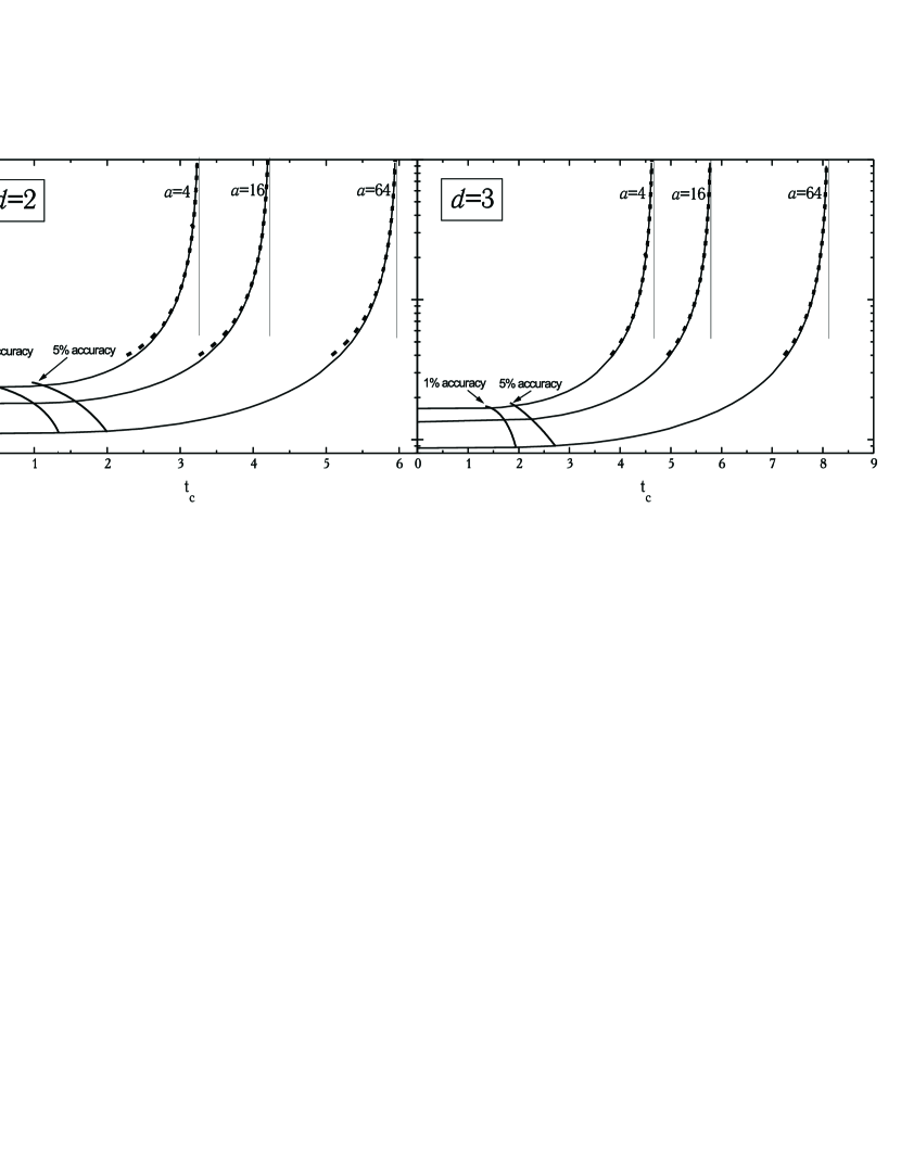
Figure 2: The dependencies of the critical mass $m_{c}$ on the critical temperature $t_{c}$ for the three values of the parameter $a$: $a=4$, $a=16$, $a=64$. The logarithmic scale for $m_{c}$ is used. The left and the right panels show $m_{c}(t_{c})$ for 2D and 3D, respectively. The solid lines show the result of quantum MF approach (6), the vertical lines are the classical MF limits [3, 4] the dashed lines are the first quantum correction (10). The lines marked as 1% and 5% show the estimations for the domains, where the ”quantum limit” value of $m_{c}(t=0)$ delivers the corresponding accuracy for $m_{c}(t)$.

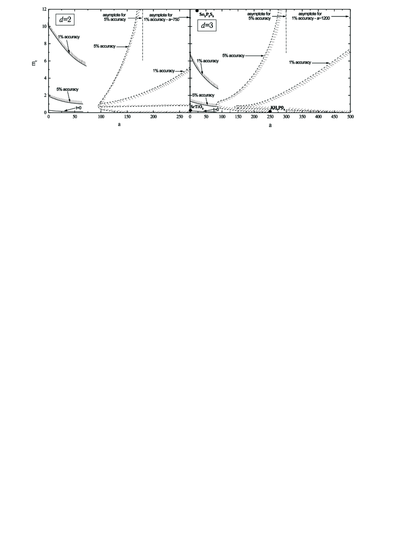
Figure 3: The phase diagram for the limit domains of 2D and 3D systems (the left and the right panel, respectively). Solid lines indicate the classical limit $m\to+\infty$ (hatching on these curves indicates the beginning of the classical area with an accuracy of 1% and 5%). The purely quantum limit corresponds to the curve with $t=0$ (the domain of applicability for this limit is shown in Fig.2). The dashed lines indicate the order-disorder limit area. Vertical lines are the classical asymptotes for these curves. The displacive limit approximately corresponds to $a<1$. Points on the right panel are the estimations for $m$ and $a$ from the known experimental data for Sn₂P₂S₆, SrTiO₃, and KH₂PO₄.

References

- [1] Zhong W and Vanderbilt D 1996 Phys. Rev. B 53 5047.
- [2] Bruce A D and Cowley R A 1981 Structural Phase Transition (Taylor and Francis Ltd. London).
- [3] Rubtsov A N, Hlinka J and Janssen T 2000 Phys. Rev. E 61 126.
- [4] Savkin V V and Rubtsov A N 2000 JETP 91 1204.
- [5] Perez-Mato J M and Salje E K H 2000 Journal of Phys.: Condensed Matter 12 L29.
- [6] Prosandeev S A, Trepakov V A, Savinov M E and Kapphan S E 2001 Journal of Phys.: Condensed Matter 13 1.
- [7] Elliott R J and Wood C 1971 J. Phys. C 4 2359.
- [8] Elliott R J and Wood C 1971 J. Phys. C 4 2370.
- [9] Ristig M L and Kim J W 1996 Phys. Rev. B 53 6665.
- [10] Wang Y-L and Cooper B R 1968 Phys. Rev. 172 539.
- [11] Shender E F 1974 JETP 66 2198.
- [12] Irkhin V Yu and Katanin A A 1998 Phys. Rev. B 58 5509.
- [13] Kim J W, Ristig M L and Clark J W 1998 Phys. Rev. B 57 56.
- [14] Rubtsov A N and Janssen T 2001 Phys. Rev. B 63 172101.
- [15] Landau L D and Lifshitz E M 1977 Statistical Physics (Pergamon Press, Oxford).
- [16] Il’inskii Yu A and Keldysh L V 1994 Electromagnetic Responce of Material Media (Plenum Press, New York).
- [17] Kalitkin N N 1976 Numerical methods (Nauka, Moscow, in Russian).
- [18] Toral R and Chakrabarti A 1990 Phys. Rev. B 42 2445.
- [19] Feynman R and Hibbs A R 1965 Quantum Mechanics and Path Integrals (McGraw-Hill, New York)
- [20] Vysochanskii Yu V and Slivka V Yu 1994 Ferroelectrics of the Sn2P2S6 family. Properties in the vicinity of Lifshitz point (Lvov, in Russian).
- [21] Barsamian T K, Khasanov S S and Shekhman V Sh 1993 Ferroelectrics 138 63.
- [22] Hlinka J, Janssen T and Dvorak V 1999 J. Phys.: Cond. Matter 11 3209
- [23] Scott B, Pressprich M, Willet R D and Clearly D A 1992 J. Solid State Chemistry 96 294.
- [24] Christen H M, Mannhart J, Williams E J and Gerber Ch 1994 Phys. Rev. B 49 12095.
- [25] Grupp D E and Goldman A M 1997 Phys. Rev. Lett. 78 3511.
- [26] Kubo M, Oumi Y, Miura R, Stirling A, Miyamoto A, Kawasaki M, Yoshimoto M and Koinuma H 1997 Phys. Rev. B 56 13535.
- [27] Vaks V G 1973 Introduction in the microscopic theory of ferroelectrics (Nauka, Moscow, in Russian).
- [28] Itoh M, Wang R, Inaguma Y, Yamaguchi T, Shan Y-J and Nakamura T 1999 Phys. Rev. Lett. 82 3540.
- [29] Vysochanskii Yu 1998 Ferroelectrics 218 275.
- [30] Savkin V V and Rubtsov A N 2001 Surf. Sci. to be published.