A quantitative model of trading and price formation in financial markets

Abstract

We use standard physics techniques to model trading and price formation in a market under the assumption that order arrival and cancellations are Poisson random processes. This model makes testable predictions for the most basic properties of a market, such as the diffusion rate of prices, which is the standard measure of financial risk, and the spread and price impact functions, which are the main determinants of transaction cost. Guided by dimensional analysis, simulation, and mean field theory, we find scaling relations in terms of order flow rates. We show that even under completely random order flow the need to store supply and demand to facilitate trading induces anomalous diffusion and temporal structure in prices.

There have recently been efforts to apply physics methods to problems in economics Mantegna00 ; Bouchaud00 . This effort has yielded interesting empirical analyses and conceptual models. However, with the exception of refinements to option pricing theory, so far it has had little success in producing theories that make falsifiable predictions about markets. In this paper we develop a mechanistic model of a standard method for trade matching in order to make quantitative predictions about the most basic properties of markets. This model differs from standard models in economics in that we make no assumptions about agent rationality. The model makes falsifiable predictions based on parameters that can all be measured in real data, and preliminary results indicate that it has substantial explanatory power Daniels02

The random walk model was originally introduced by Bachelier to describe prices, five years before Einstein used it to model Brownian motion Bachelier00 . Although this is one of the most widely used models of prices in financial economics, there is still no understanding of its most basic property, namely, its diffusion rate. We present a theory for how the diffusion rate of prices depends on the flow of orders into the market, deriving scaling relations based on dimensional analysis, mean field theory, and simulation. We also make predictions of other basic market properties, such as the gap between the best prices for buying and selling, the density of stored demand vs. price, and the impact of trading on prices.

Most modern financial markets operate continuously. The mismatch between buyers and sellers that typically exists at any given instant is solved via an order-based market with two basic kinds of orders. Impatient traders submit market orders, which are requests to buy or sell a given number of shares immediately at the best available price. More patient traders submit limit orders, which also state a limit price, corresponding to the worst allowable price for the transaction. Limit orders often fail to result in an immediate transaction, and are stored in a queue called the limit order book. Buy limit orders are called bids, and sell limit orders are called offers or asks. We will label the logarithm of the best (lowest) offering price $a(t)$ and the best (highest) bid price $b(t)$. There is typically a non-zero price gap between them, called the spread $s(t)=a(t)-b(t)$.

As market orders arrive they are matched against limit orders of the opposite sign in order of price and arrival time. Because orders are placed for varying numbers of shares, matching is not necessarily one-to-one. For example, suppose the best offer is for 200 shares at $60 and the the next best is for 300 shares at $60.25; a buy market order for 250 shares buys 200 shares at $60 and 50 shares at $60.25, moving the best offer $a(t)$ from $60 to $60.25. A high density per price of limit orders results in high liquidity for market orders, i.e., it implies a small price movement when a market order of a given size is placed.

We analyze the queueing properties of such order-matching algorithms with the simple random order placement model shown in Fig. 1.

Figure 1: Schematic of the order-placement process. Stored limit orders are shown “stacked” along the price axis, with bids (buy limit orders) negative and offers (sell limit orders) positive. New limit orders are visualized as “falling” randomly onto the price axis. New offers can be placed at any price greater than the best bid, and new bids can be placed at any price less than the best offer. Limit orders can be removed by random spontaneous deletion or by market orders of the opposite sign.

All the order flows are modeled as Poisson processes. We assume that market orders in chunks of $\sigma$ shares arrive at a rate of $\mu$ shares per unit time, with an equal probability for buy orders and sell orders. Similarly, limit orders in chunks of $\sigma$ shares arrive at a rate of $\alpha$ shares per unit price and per unit time. Offers are placed with uniform probability at integer multiples of a tick size $dp$ in the range $b(t)<p<\infty$, and similarly for bids on $-\infty<p<a(t)$. $p$ represents the logarithm of the price, and $dp$ is a logarithmic price interval . (To avoid repetition the word price will henceforth refer to the logarithm of price.) When a market order arrives it causes a transaction. Under the assumption of constant order size, a buy market order removes an offer at price $a(t)$, and a sell market order removes a bid at price $b(t)$. Alternatively, limit orders can be removed spontaneously by being canceled or by expiring. We model this by letting any order be removed randomly with constant probability $\delta$ per unit time.

This order placement process is designed to permit an analytic solution. The model builds on previous work modeling the continuous double auction Domowitz94 ; Bollerslev94 ; Eliezer98 ; Maslov00 ; Iori01 ; Challet01 ; Slanina01 . While the assumption of limit order placement over an infinite interval is clearly unrealistic Bouchaud02 ; Zovko02 , it provides a tractable boundary condition for modeling the behavior of the limit order book in the region of interest, near the midpoint price $m(t)=(a(t)+b(t))/2$. It is also justified because limit orders placed far from the midpoint usually expire or are canceled before they are executed. For our analytic model we use a constant order size $\sigma$. In simulations we also use variable order size, e.g. half-normal distributions with standard deviation $\sqrt{2/\pi}\sigma$, which gives similar results.

For simplicity in our model we do not directly allow limit orders that cross the best price. For example, a buy order of size $x+y$ may have a limit price that is higher than the best ask, so that $x$ shares immediately result in a trade, and $y$ shares remain on the book. Such an order is indistinguishable from a market order for $x$ shares immediately followed by a non-crossing limit order for $y$ shares. By definition our model implicitly allows such events, though it neglects the resulting correlation in order placement.

Dimensional analysis simplifies this problem and provides rough estimates of its scaling properties. The three fundamental dimensions are shares, price, and time. There are five parameters: three order flow rates and two discreteness parameters. The order flow rates are $\mu$, the market order arrival rate, with dimensions of shares per time; $\alpha$, the limit order arrival rate per unit price, with dimensions of shares per price per time; and $\delta$, the rate of limit order decays, with dimensions of 1/time. The two discreteness parameters are the price tick size $dp$, with dimensions of price, and the order size $\sigma$, with dimensions of shares. Because there are five parameters and three dimensions, and because the dimensionality of the parameters is sufficiently rich, all the properties of the limit-order book can be described by functions of two independent parameters.

We perform the dimensional reduction by taking advantage of the fact that the effect of the order flow rates is primary to that of the discreteness parameters. This leads us to construct nondimensional units based on the order flow parameters alone, and take nondimensionalized versions of the discreteness parameters as the independent parameters whose effects remain to be understood. There are three order flow rates and three fundamental dimensions. Temporarily ignoring the discreteness parameters, there are unique combinations of the order flow rates with units of shares, price, and time. These define a characteristic number of shares $N_{c}=\mu/2\delta$, a characteristic price interval $p_{c}={\mu}/2{\alpha}$, and a characteristic timescale $t_{c}=1/\delta$. (The factors of two are a matter of convenience; they occur because we have defined the market order rate for either a buy or a sell order to be $\mu/2$.) These characteristic values can be used to define nondimensional coordinates $\hat{p}=p/p_{c}$ for price, $\hat{N}=N/N_{c}$ for shares, and $\hat{t}=t/t_{c}$ for time.

A nondimensional scale parameter based on order size is constructed by dividing the typical order size $\sigma$ (which is measured in shares) by the characteristic number of shares $N_{c}$, i.e. $\epsilon\equiv\sigma/N_{c}=2\delta\sigma/{\mu}$. $\epsilon$ characterizes the granularity of the orders stored in the limit order book. A nondimensional scale parameter based on tick size is constructed by dividing by the characteristic price, i.e. $dp/p_{c}=2{\alpha}dp/{\mu}$. The theoretical analysis and the simulations show that there is a sensible continuum limit as the tick size $dp\rightarrow 0$, in the sense that there is non-zero price diffusion and a finite spread. Furthermore, the dependence on tick size is usually weak, and for many purposes the limit $dp\rightarrow 0$ approximates the case of finite tick size fairly well.

Space constraints do not permit us to review the theoretical development of the model in this Letter; it is presented in detail in Ref. Smith02 . We write an approximate master equation for the number of shares at each price level $p$ at time $t$, and then find a self-consistent mean field theory steady-state solution. We also develop an independent interval approximation, borrowing methods from the study of reaction-diffusion equations Majumdar00 . We find that the theory fits the simulation results accurately for large values of $\epsilon$. For small values of $\epsilon$ the theory continues to capture the mean spread very well. The predictions of other properties remain qualitatively correct, but are no longer quantitatively accurate. The results we quote here are all from simulations; to see the development of the theory and comparisons to simulation, see ref. Smith02 .

In the following we explore the predictions of the model for the basic properties of markets. As already noted, neglecting the effects of the discreteness parameters, gives three dimensional quantities and three parameters, which we call the continuum approximation. For the continuum approximation dimensional analysis alone yields simple estimates for the most relevant economic properties of the models. We have refined these estimates by simulation and mean field theory, which take the effects of $\epsilon$ and $dp/p_{c}$ into account. The results are summarized in Table 1, and described in more detail below.

Quantity	Dimensions	Continuum scaling relation	Scaling from simulation and theory
Asymptotic depth	$shares/price$	$d\sim\alpha/\delta$	$d=\alpha/\delta$
Spread	$price$	$s\sim\mu/\alpha$	$s=(\mu/\alpha)f(\epsilon,dp/p_{c})$
Slope of depth profile	$shares/price^{2}$	$\lambda\sim\alpha^{2}/\mu\delta=d/s$	$\lambda=(\alpha^{2}/\mu\delta)g(\epsilon,dp/p_{c})$
Price diffusion rate	$price^{2}/time$	$D\sim\mu^{2}\delta/\alpha$	($\tau\rightarrow 0$, $dp\rightarrow 0$)  $D_{0}\sim\mu^{2}\delta/\alpha\epsilon^{-0.5}$
			($\tau\rightarrow\infty$, $dp\rightarrow 0$) $D_{\infty}\sim\mu^{2}\delta/\alpha\epsilon^{0.5}$

Table 1: Predictions of scaling of market properties vs. order flow. The third column contains predictions from the continuum analysis, in which the discreteness parameters are ignored, and the fourth column gives more accurate predictions from theory and simulation. The functions $f$ and $g$ are the order of magnitude of one throughout the relevant ranges of variation of $\epsilon$ and $dp/p_{c}$.

The bid-ask spread is the difference between the best price for buying and selling. It is an important determinant of transaction costs, as it is the price that one pays to buy a share and then immediately sell it. The spread has dimensions of price and therefore scales under the continuum approximation as $\mu/\alpha$. Simulations and theory show that the spread varies as $(\mu/\alpha)f(\epsilon,dp/p_{c})$, where $f$ is a fairly flat function with $f(\epsilon,dp/p_{c})\approx 1/2$ across much of the range of interest (see ref. Smith02 ).

Another interesting quantity is the average depth profile $n(p)=\langle n(p,t)\rangle$, which is the density of shares per price interval. The average depth profile is relatively small near the midpoint and increases to an aysymptotic value far from the midpoint, as shown in Fig. 2.

Figure 2: The mean depth profile versus price in nondimensional coordinates $\hat{n}=np_{c}/N_{c}=n\delta/\alpha$ vs. $\hat{p}=p/p_{c}=2\alpha p/\mu$. The origin $p/p_{c}=0$ corresponds to the midpoint. We show three different values of the nondimensional granularity parameter: $\epsilon=0.2$ (solid), $\epsilon=0.02$ (dash), $\epsilon=0.002$ (dot), all with tick size $dp=0$.

The approach to an asymptotic value is a consequence of our assumption of uniform order placement over an infinite range, and is not realistic. It should be viewed as a convenient boundary condition for understanding the depth near $\hat{p}=0$, where transactions occur. From dimensional analysis the asymptotic depth, which has units of shares/price is $\alpha/\delta$. This result is exact.

An important property of the depth profile is its slope near the origin, which determines the price response to the placement of a small market order. From continuum dimensional analysis the slope of the average depth profile scales as $\lambda\sim\alpha^{2}/\mu\delta$. This is altered by effects due to the granularity of orders. For large $\epsilon$ the depth profile is a concave function with nonzero values at $\hat{p}=0$, whereas for small $\epsilon$, $n(0)\approx 0$ and $n(\hat{p})$ is convex near $\hat{p}=0$.

In addition to the spread, the price response for executing a market order is also a key factor determining transaction costs. It can be characterized by a price impact function $\Delta p=\phi(\omega,\tau,t)$, where $\Delta p$ is the price shift at time $t+\tau$ caused by a market order $\omega$ at time $t$. Price impact causes market friction, since selling tends to drive the price up and buying tends to drive it down, so executing a circuit causes a loss. (This loss, from changing the order distribution, is in addition to the intrinsic loss created by a nonzero spread.) The price impact is closely related to the demand function, providing a natural starting point for theories of statistical or dynamical properties of markets Farmer98 ; Bouchaud98 . A naive argument predicts that the price impact $\phi(\omega)$ should increase at least linearly: Fractional price changes should not depend on the scale of price. Suppose buying a single share raises the price by a factor $k>1$. If $k$ is constant, buying $\omega$ shares in succession should raise it by $k^{\omega}$. Thus, if buying $\omega$ shares all at once affects the price at least as much as buying them one at a time, the ratio of prices before and after impact should increase at least exponentially. Taking logarithms implies that the price impact as we have defined it above should increase at least linearly. In contrast, from empirical studies $\phi(\omega)$ for buy orders grows more slowly than linearly Hausman92 ; Farmer96 ; Torre97 ; Kempf98 ; Plerou01 . A recent more accurate study by Lillo et al. demonstrates that for the New York Stock Exchange $\phi$ is strongly concave, and that in general a simple power law of the form $\phi(\omega)\sim\omega^{\beta}$ is not a good approximation Lillo02 .

Our model gives average instantaneous price impact functions $\Delta p=\langle\phi(\omega,0,t)\rangle$ as shown in Fig. 3.

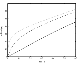
Figure 3: The average price impact corresponding to the results in Fig. (2). The average instantaneous movement of the nondimensional mid-price, $\langle dm\rangle/p_{c}$ caused by an order of size $N/N_{c}=N\epsilon/\sigma$. $\epsilon=0.2$ (solid), $\epsilon=0.02$ (dash), $\epsilon=0.002$ (dot).

The price impact approaches a linear function for large $\epsilon$, but for smaller values of $\epsilon$ it is strongly concave, particularly near the midpoint. Plotting this on log-log scale, this function does not follow a pure power law. For example, for $\epsilon=0.002$, the exponent is $\beta\approx 0.5$ for small orders, and $\beta\approx 0.2$ for larger orders. This is in agreement with the results of Lillo et al. Lillo02 . The instantaneous price impact $\phi(\omega,0,t)$ can be understood in terms of the depth profile $n(p,t)$, as explained in ref. Smith02 .

The price diffusion rate is a property of central interest. In finance, it is typically characterized in terms of the standard deviation of prices at a particular timescale, which is referred to as volatility. Volatility is a measure of the uncertainty of price movements and is the standard way to characterize risk. In Fig. 4 we plot simulation results for the

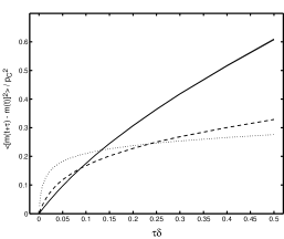
Figure 4: The variance of the change in the nondimensionalized midpoint price versus the nondimensional time lag. For a pure random walk this would be a straight line whose slope is the diffusion rate, which is proportional to the square of the volatility. The fact that the slope is steeper for short times comes from the nontrivial temporal persistence of orders. The three cases correspond to Fig. 2: $\epsilon=0.2$ (solid), $\epsilon=0.02$ (dash), $\epsilon=0.002$ (dot).

variance of the change in the midpoint price at timescale $\tau$, i.e. the variance of $m(t+\tau)-m(t)$. The slope is the diffusion rate, which at any fixed timescale is proportional to the square of the volatility. It appears that there are at least two timescales involved, with a faster diffusion rate for short timescales and a slower diffusion rate for long timescales. Such correlated diffusion is not predicted by mean-field analysis. Simulation results show that the diffusion rate is correctly described by the product of the estimate from continuum dimensional analysis $\mu^{2}\delta/{\alpha}^{2}$, and a $\tau$-dependent power of the nondimensional granularity parameter $\epsilon=2\delta\sigma/\mu$, as summarized in table 1. We cannot currently explain why this power is $-1/2$ for short term diffusion and $1/2$ for long-term diffusion.

This model contains numerous simplifying assumptions. Nevertheless, it is the very simplicity of this model that allows us to make unambiguous predictions about the most basic properties of real markets. Our prediction for the price impact function agrees with the best empirical measurements and suggests that concavity is a robust feature deriving from institutional structure, rather than rationality Lillo02 . Preliminary analysis of data from the London Stock Exchange using the nondimensional coordinates defined here shows an even better collapse of the price impact function, suggesting the existence of universal supply and demand functions. Futhermore, the results indicate that scaling relationships along the lines that we predict have remarkable explanatory value for both the spread and the price diffusion rate Daniels02 . Even though we do not expect the predictions of this model to be exact in every detail, they provide a simple benchmark that can guide future improvements. Our model illustrates how the need to store supply and demand gives rise to interesting temporal properties of prices and liquidity even under assumptions of perfectly random order flow, and demonstrates the importance of making realistic models of market mechanisms.

- (1) , R.N. Mantegna and H.E. Stanley, An Introduction to Econophysics: Correlations and Complexity in Finance, Cambridge University Press (2000).
- (2) , J.-P. Bouchaud and M. Potters, Theory of Financial Risk, Cambridge University Press (2000).
- (3) M. Daniels, J.D. Farmer, L. Gillemot, P. Patelli, E. Smith, and I. Zovko, “Predicting the spread, volatility, and price impact based on order flow: The London Stock Exchange”, preliminary manuscript.
- (4) L. Bachelier, “Théorie de la spéculation”, 1900. Reprinted in P.H. Cootner, The Random Character of Stock Prices, MIT Press Cambridge (1964).
- (5) I. Domowitz and Jianxin Wang, “Auctions as algorithms”, J. of Econ. Dynamics and Control 18, 29 (1994).
- (6) T. Bollerslev, I. Domowitz, and J. Wang, “Order flow and the bid-ask spread: An empirical probability model of screen-based trading”, J. of Econ. Dynamics and Control 21, 1471 (1997).
- (7) D. Eliezer and I.I. Kogan, “Scaling laws for the market microstructure of the interdealer broker markets”, http://xxx.lanl.gov/cond-mat/9808240.
- (8) S. Maslov, “Simple model of a limit order-driven market”, Physica A 278, 571(2000).
- (9) G. Iori and C. Chiarella, “A simple microstructure model of double auction markets”, Kings College preprint, 2001.
- (10) F. Slanina, “Mean-field approximation for a limit order driven market model”, http://xxx.lanl.gov/cond-mat/0104547
- (11) D. Challet and R. Stinchcombe, “Analyzing and Modelling 1+1d markets”, Physica A 300, 285, (2001), preprint cond-mat/0106114
- (12) S.N. Majumdar, S. Krishnamurthy, and M. Barma, J. Stat. Phys. 99, 1 (2000)
- (13) Eric Smith, J. Doyne Farmer, László Gillemot, and Supriya Krishnamurthy, “Statistical theory of the continuous double auction”, xxx.lanl.gov/cond-mat/0210475.
- (14) J.D. Farmer, “Market force, ecology, and evolution”, SFI working paper 98-12-117 or http://xxx.lanl.gov/adapt-org/9812005.
- (15) J.-P. Bouchaud and R. Cont, European Physics Journal B 6, 543 (1998)
- (16) J.A. Huasman and A.W. Lo, “An ordered probit analysis of transaction stock prices”, Journal of Financial Economics, 31 319-379 (1992)
- (17) J.D. Farmer, “Slippage 1996”, Prediction Company internal technical report (1996), http://www.predict.com/jdf/slippage.pdf
- (18) N. Torre, BARRA Market Impact Model Handbook, BARRA Inc, Berkeley CA, www.barra.com (1997).
- (19) A. Kempf and O. Korn, “Market depth and order size”, University of Mannheim technical report (1998).
- (20) V. Plerou, P. Gopikrishnan, X. Gabaix, and H.E. Stanley, “Quantifying stock price response to demand fluctuations”, xxx.lanl.gov/cond-mat/0106657.
- (21) F. Lillo, J.D. Farmer, and R. Mantegna, “Single curve collapse of the price impact function for the New York Stock Exchange”, xxx.lanl.gov/cond-mat/0207428, to appear in Nature.
- (22) J.-P.Bouchaud, M.Mezard, and M.Potters, Statistical properties of the stock order books: Empirical results and models, xxx.lanl.gov/cond-mat/0203511.
- (23) I. Zovko and J.D. Farmer, “The power of patience: A behavioral regularity in limit order placement”, xxx.lanl.gov/cond-mat/0206280.