Fluctuation-dissipation ratio of a spin glass in the aging regime

Abstract

We present the first experimental determination of the time autocorrelation $C(t^{\prime},t)$ of magnetization in the non-stationary regime of a spin glass. Quantitative comparison with the response, the magnetic susceptibility $\chi(t^{\prime},t)$, is made using a new experimental setup allowing both measurements in the same conditions. Clearly, we observe a non-linear fluctuation-dissipation relation between $C$ and $\chi$, depending weakly on the waiting time $t^{\prime}$. Following theoretical developments on mean-field models, and lately on short range models, it is predicted that in the limit of long times, the $\chi(C)$ relationship should become independent on $t^{\prime}$. A scaling procedure allows us to extrapolate to the limit of long waiting times.

Almost half a century ago, derivation of the fluctuation dissipation theorem (FDT) Callen ; Kubo which links the response function of a system to its time autocorrelation function, made it possible to work out dynamics from the knowledge of statistical properties at equilibrium. Nevertheless, this progress was limited by severe restrictions. FDT applies only to ergodic systems at equilibrium. Yet, such systems represent a very limited part of natural objects, and there is now a growing interest on non-ergodic systems and on the related challenging problem of the existence of fluctuation dissipation (FD) relations valid in off-equilibrium situations.

A way to extend equilibrium concepts to non-equilibrium situations is to consider systems in which single time dependent quantities (like the average energy) are near equilibrium values though quantities which depend on two times (like the response to a field) are not. Spin glasses Binder are such systems. They remain strongly non-stationary even when their rate of energy decrease has reached undetectable values. In the absence of any external driving force, they slowly evolve towards equilibrium, but never reach it, even on geological time-scales. In these conditions, FDT is not expected to hold. A quite general FD relation can be written as CuKu2 ; CuKu3 $R(t^{\prime},t)=\beta X(t^{\prime},t)\partial C(t^{\prime},t)/\partial t^{\prime}$, where $R(t^{\prime},t)$ is the impulse response of an observable to its conjugate field, $C(t^{\prime},t)$ the autocorrelation function of the observable and $\beta={1/k_{B}T}$. FDT corresponds to $X=1$. Determination of $X$, the fluctuation-dissipation ratio (FDR), or of an “effective temperature”, $T_{eff}=T/X$, is the aim of many recent theoretical studies which predicted a generalization of FDT CuKu1 ; CuKu2 ; CuKu3 in “weak ergodicity breaking” systems Bouchaud . In the asymptotic limit of large times, it is conjectured that the FDR should depend on time only through the correlation function: $X(t^{\prime},t)=X(C(t^{\prime},t))$ for $t^{\prime}$ (and $t>t^{\prime}$) $\rightarrow\infty$. The dependence of $X$ on $C$ would reflect the level of thermalization of different degrees of freedom within different timescales CuKu3 . Thus, the integrated forms of the FD relation would become $\chi(t^{\prime},t)=\beta\int_{C(t^{\prime},t)}^{C(t,t)}X(C)dC$ (susceptibility function) and $\sigma(t^{\prime},t)=\beta\int_{0}^{C(t^{\prime},t)}X(C)dC$ (relaxation function). They would depend on $t$ and $t^{\prime}$ only through the value of $C$. The field cooled magnetization would read $\chi_{FC}=\beta\int_{0}^{C(t,t)}{X(C)dC=\beta(1-\int_{0}^{1}{C(X)dX)}}$ (in the simplest Ising case with $C(t,t)=1$), formally equivalent to the Gibbs equilibrium susceptibility in the Parisi replica symmetry breaking solution for the Sherrington-Kirkpatrick model Mezard , with $C\Leftrightarrow q$ (overlap between pure states) and $X\Leftrightarrow x$ (repartition of overlap). Theoretical attempts, analytical Franz (with the constraint of stochastic stability) and numerical Marinari (with the problems of size effects), were made in order to confirm the above properties in short range models. Up to now, experimental investigations correspond only to the quasi-stationary regime Grigera or are very indirect CuGre .

Here we report the result of an investigation of FD relation in the insulating spin glass CdCr_1.7In_0.3S₄ Alba , an already very well known compound, with $T_{g}=16.2K$. Above $T_{g}$, the susceptibility follows a Curie-Weiss law $\chi=\mathcal{C}/(T-\Theta)$ where $\mathcal{C}$ corresponds to ferromagnetic clusters of about 50 spins, and $\Theta\approx-9K$ Vincent1 . The sample is a powder with grain sizes around $10\,\mu m$, embedded in silicon grease to insure good thermal contact between grains, and compacted into a coil foil cylindrical sample holder $5\,mm$ wide and $40\,mm$ long. The two times dependence of the magnetic relaxation (TRM) of this compound was extensively studied Vincent2 .

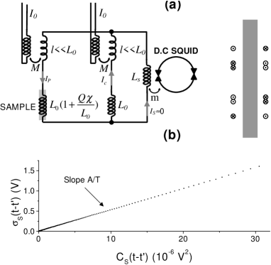
Figure 1: a) Schematic of the detection circuit. The pick-up coil (right side), containing the cylindrical sample, is a third order gradiometer made of +3 -6 +6 -3 turns. b) Calibration is obtained by measuring relaxation versus correlation in a high conductivity copper sample at equilibrium at $4.2K$.

In principle, SQUID measurement of magnetic fluctuations is very simple Ocio ; Refregier1 . The difficulty lies in the extreme weakness of the thermodynamic fluctuations (of the order of the response to a field about $10^{-7}\mathrm{G}$ in our case). Therefore, the setup is carefully screened against stray fields by superconducting shields, strict precautions are taken to suppress spurious drifts of the SQUID electronics, and the pick-up coil is a third order gradiometer. The result is that the proper noise power spectrum of the system without sample allows time analysis of the magnetic fluctuations signal over up to 2000 s of sample fluctuations with more than 20 dB of signal/noise ratio. Moreover, in the non-stationary regime, the time autocorrelation of magnetic fluctuations $C(t^{\prime},t)=\frac{1}{N}\sum_{i}\left<\mathbf{m}_{i}(t^{\prime})\mathbf{m}_{i}(t)\right>$, where $\mathbf{m}_{i}$ is the elementary moment at site $i$, must be determined as an ensemble average over a large number of records of the fluctuation signal, each one initiated by a quench from above $T_{g}$ (“birth” of the system). And finally, we want to compare quantitatively correlation and relaxation data. The relaxation function $\sigma(t^{\prime},t)=\frac{1}{N}\sum_{i}\left<\mathbf{m}_{i}(t)\right>/\mathbf{H}_{i}$ is measured by cooling the sample at time zero from above $T_{g}$ to the working temperature in a small field, turning off the field at time $t^{\prime}$ and recording the magnetization at further times $t$. Using a classical magnetometer with homogeneous field, quantitative comparison between $C$ and $\sigma$ is almost impossible due to the strong discrepancy between the coupling factors in both experiments. Therefore, we have developed a new bridge setup depicted in Fig.1a, allowing measurements of both fluctuations and response. The pick up (PU) coil of self inductance $L_{0}$ is connected to the input coil of a SQUID, of self inductance $L_{S}$. The whole circuit is superconducting. Relaxation measurements use a small coil $l$ inserted in the pick-up circuit, and coupled inductively with mutual inductance $M$ to an excitation winding. A current $I_{0}$ injected in the excitation results in a field induced by the PU coil itself ($\leqslant 1\mathrm{mG}$ here, clearly in the linear regime though inhomogeneous), and the sample response is measured by the SQUID. To get rid of the term $L_{0}$, the sample branch is balanced by a similar one without sample, excited oppositely (see Fig.1a). The flux delivered to the PU by an elementary moment $\mathbf{m}$ at position $\mathbf{r}$ is given by $\Phi(t)=\mathbf{m}(\mathbf{r},t)\mathbf{h}(\mathbf{r})$ where $\mathbf{h}$ is the magnetic field produced by a unit of current flowing in the PU. Flux conservation in the PU circuit results in a current $I_{S}$ flowing in the input coil of the SQUID whose output voltage is $V_{S}=GI_{S}$. Detailed analysis of the system will be published elsewere. The main features are as follows.

As the fluctuations of elementary moments in the sample are homogeneous and spatially uncorrelated at the scale of the PU, the SQUID output voltage autocorrelation is given by:

$$C_{S}(t^{\prime},t)=\langle V_{S}(t^{\prime})V_{S}(t)\rangle=C(t^{\prime},t)Q\frac{G^{2}}{{(L_{0}+2L_{S})^{2}}}$$ (1)

$Q=\sum_{i}{\mathbf{h}^{2}(\mathbf{r}_{i})}$ where the index $i$ refers to a moment site, is the coupling factor to the PU, including demagnetizing field effects since $\mathbf{h}$ is the internal field.

The elementary moment response at site $i$ is $R_{i}(t^{\prime},t)={\partial\left\langle{\mathbf{m}_{i}(t)}\right\rangle}/{\partial\mathbf{h}(\mathbf{r}_{i},t^{\prime})}$.Taking into account that the medium is homogeneous, the relaxation function of the SQUID output voltage is given by

$$\sigma_{S}(t^{\prime},t)=\frac{V_{S}(t^{\prime},t)}{I_{0}}=\sigma(t^{\prime},t)Q\frac{MG}{L_{0}(L_{0}+2L_{S})}.$$ (2)

Thus, the coupling factor $Q$ disappears in the relation between $C_{S}$ and $\sigma_{S}$, independently on the nature and shape of the sample. There remains only the inductance terms $M$, $L_{0}$ and $L_{S}$. These being difficult to determine with enough accuracy, absolute calibration was performed using a copper sample of high conductivity, by measuring $\sigma_{S}(t^{\prime},t)$ and $C_{S}(t^{\prime},t)$ — computed by standard fast Fourier transform algorithm — at $4.2\mathrm{K}$ (⁴He boiling temperature at normal pressure): with this ergodic material, the relation between both measured quantities is linear with slope $A/T$, where $A$ is the sample independent calibration factor (see Fig.1b). From the knowledge of $A$, determined at $4.2\mathrm{K}$, the system is equivalent to a thermometer, i.e. the FDT slope is known exactly at any temperature.

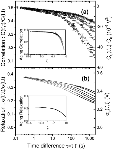
Figure 2: Aging and scaling of (a) correlation (b) relaxation at $T=0.8T_{g}$. Both are measured for waiting times $t^{\prime}=100$ ($\circ$), 200 ($\triangle$) , 500($\triangledown$), 1000($\diamond$), 2000 ($+$) , 5000($\times$), 10000($*$) seconds from bottom to top. Reported error-bars on correlation have a length of two standard-deviation, corresponding to averages over records. In insets, scaling of the aging parts versus $\zeta=(t^{1-\mu}-t^{\prime 1-\mu})/(1-\mu)$, using $\mu=0.87$. The stationary parts are found to obey a power-law decrease with an exponent $\alpha=0.05$.

In the spin glass sample, $C_{S}(t^{\prime},t)$ and $\sigma_{S}(t^{\prime},t)$ were measured at $T=0.8T_{g}$ after quench from a temperature $T\approx 1.2T_{g}$. To get a precise definition of the “birth” time, a minimum value of 100 s was chosen for $t^{\prime}$. The autocorrelation was determined from an ensemble of 320 records of $12000\,\mathrm{s}$ of the fluctuation signal. The ensemble averages were computed in each record from the signal at $t^{\prime}$, averaged over $\delta t^{\prime}\leqslant t^{\prime}/20$, and the one at $t$, averaged over $\delta t\leqslant(t-t^{\prime})/10$ — the best compromise allowing a good average convergence still being compatible with the non-stationarity — , and averaging over all records. As there is an arbitrary offset in the SQUID signal, the connected correlation was computed. Nevertheless, this was not enough to suppress the effect of spurious fluctuation modes of period much longer than 2000 s, giving a non-zero average offset on the correlation results. Thus, as a first step, we have plotted all correlation data, taking as the origin the value of $\langle V_{S}^{2}(t^{\prime})\rangle$. Due to the elementary measurement time constant this last term corresponds to an average over $t-t^{\prime}$ about $10^{-2}$s, i.e. a range of $(t-t^{\prime})/t^{\prime}$ corresponding to stationary regime. Thus, all $C_{S}$ data are shifted by a common offset $C_{0}$. The result is shown in Fig.2a (right sided scale), as a function of $t-t^{\prime}$ for values of $t^{\prime}$ from 100 s to 10000 s. Residual oscillations —and large error bars— for $t^{\prime}=100s$ reveal the limit of efficiency of our averaging procedure. Corresponding relaxation data are plotted on Fig.2b. In both results, one can see that the curves merge at low $t-t^{\prime}$ , meaning that they do not depend on $t^{\prime}$ (stationary regime). At $t-t^{\prime}\geqslant t^{\prime}$, they strongly depend on $t^{\prime}$, the slower decay corresponding to the longer $t^{\prime}$.

The correlation offset must be determined. As zero of correlation is unreachable in experimental time, correction of the offset could be obtained from the knowledge of $C(t,t)$. Nevertheless, due to clustering, $C(t,t)$ depends on temperature and cannot be determined from the high temperature susceptibility. In canonical compounds like 1% Cu:Mn Binder , with negligible clustering, the field-cooled susceptibility is temperature independent in agreement with the Parisi-Toulouse hypothesis Marinari ; Parisi , yielding $C(t,t)=T_{g}\chi_{FC}(T)$. We used a generalization of this relation with the condition that a smooth dependence of $C(t,t;T)/T$ must result Parisi2 . This was obtained by using for $T_{g}$ a slightly different value, $T_{g}^{*}=17.2\mathrm{K}$. Then, from the value of the calibration factor $A$, and writing $C(t,t;0.8T_{g})=17.2\chi_{FC}(0.8T_{g})$, $C_{S}(t,t;0.8T_{g})$ can be determined, and suppression of the offset can be performed by using the $\chi(C)$ plot, first introduced by Cugliandolo and Kurchan CuKu2 . We plot the normalized susceptibility function $\widetilde{\chi}(t^{\prime},t)=1-\widetilde{\sigma}(t^{\prime},t)$ where $\widetilde{\sigma}(t^{\prime},t)=\sigma_{S}(t^{\prime},t)/\sigma_{S}(t,t)$ (note that $\sigma(t,t)=\chi_{FC}$) versus normalized autocorrelation $\widetilde{C}(t^{\prime},t)-\widetilde{C}_{0}=(C_{S}(t^{\prime},t)-C_{0})/C_{S}(t,t;T)$ for all experimental values of $t^{\prime}$. In this graph, the FDT line has slope $-T_{g}^{*}/T$ and crosses the $\widetilde{C}$ axis at $\widetilde{C}=1$. On the data, a clear linear range appears at large $\widetilde{C}$ (small $t-t^{\prime}$), displaying the FDT slope with error $<3\%$ in the sector $\widetilde{C}\geqslant 0.47$. This allows the suppression of the correlation offset by horizontal shift of the data. The result is shown in Fig.3. It is of course based on a rough ansatz on $C(t^{\prime},t;T)$ which needs further justifications, but we stress that the induced uncertainty concerns only the position of the zero on the $\widetilde{C}$ axis, and not the shape and slope of the curves. With decreasing $\widetilde{C}$ (increasing $t-t^{\prime}\geqslant t^{\prime}$), the data points depart from the FDT line. Indeed, $\widetilde{C}(t^{\prime},t\rightarrow\infty)=0$ and $\widetilde{\chi}_{FC}=\widetilde{\chi}(t^{\prime},t\rightarrow\infty)=1$. The mean slope of the off FDT data corresponds to a temperature of about $30\mathrm{K}$. This value is far above our annealing temperature, ruling out a simple interpretation in terms of a “fictive” temperature Jackle . Despite the scatter of the results, a tendency for the data at small $t^{\prime}$ to depart the FDT line at larger values of $\widetilde{C}$ is clear: it is experimentally impossible to fulfill the condition of timescales separation underlying the existing theories . Even if the long $t^{\prime}$ limit for $\widetilde{\chi}(\widetilde{C})$ does exist, it is not reached in the plot of data in Fig.3 and a $t^{\prime}$ dependence of the $\widetilde{\chi}(\widetilde{C})$ curves is expected.

The left sided scales in Fig.2a and b correspond to $\widetilde{C}(t^{\prime},t)$ and $\widetilde{\sigma}(t^{\prime},t)$ respectively. In former works, it was shown that the whole relaxation curves could be scaled as the sum of two contributions, one stationary and one non-stationary Vincent2

$$\widetilde{\sigma}(t^{\prime},t)=(1-\Delta)(1+(t-t^{\prime})/t_{0})^{-\alpha}+\Delta\varphi(\zeta),$$ (3)

where $t_{0}$ is an elementary time of order $10^{-11}$ s, $\varphi$ is a scaling function of an effective time parameter $\zeta\propto t^{1-\mu}-t^{\prime 1-\mu}$ depending on the sub-aging coefficient $\mu<1$ Vincent2 , and $\alpha$ can be determined with good precision from the stationary power spectrum of fluctuations $S(\omega)\propto\omega^{\alpha-1}$. The inset in Fig.2b displays the result of the scaling on the relaxation curves with $\alpha=0.05$, $\Delta=0.21$ and $\mu=0.87$. As shown in the inset of Fig.2a, the scaling works rather well on the autocorrelation curves with the same exponents, but now, $q_{EA}$, the Edwards Anderson order parameter, replaces $\Delta$. We get $q_{EA}=0.37$. These results show clearly that the stationary part of the dynamics is still important yet in the aging regime, i.e. that the limit of long $t^{\prime}$ is not reached within the timescale of our experiments (in fact, timescale separation is realized if $t^{\prime}\geqslant\tau$ where $\tau$ is the observation time such that $C_{stat}(\tau)\ll q_{EA}$).

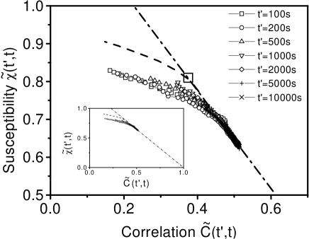
Figure 3: FD-plot. Relaxation measurements are plotted versus correlation functions for each $t^{\prime}$. The dot-dashed line (FDT line) is calculated for $T=0.8Tg=13.3K$, from the calibration obtained with the copper sample. The dashed line represents the scaling extrapolation for $t^{\prime}\rightarrow\infty$. The branching point with the FDT line, corresponds to $\widetilde{C}=q_{EA}$ (square symbol, with size giving the error range). In Inset, the same data in the whole range.

If granted, the scaling gives the long time limit of the non-stationary part of the dynamics, allowing a plot of the long times asymptotic non-stationary part of the $\widetilde{\chi}(\widetilde{C})$ curve. Of course, here we verify it only over 2 decades of time, up to $t^{\prime}=10000\,\mathrm{s}$, but it was proven to be relevant on TRM up to $t^{\prime}=100000\,\mathrm{s}$ Alba . The dashed line in Fig.3 is obtained by plotting the smoothed curves of aging parts of $\widetilde{\chi}(\zeta)$ versus $\widetilde{C}(\zeta)$. According to theoretical conjectures, $d\widetilde{\chi}(\widetilde{C})/d\widetilde{C}$ would represent the static quantity $x(q)$ Franz . One can see that the curve does not point exactly towards $\widetilde{\chi}=1$ but about 5% below. Therefore i) either the ansatz used to determine $C(t,t;T)$ is not realistic enough, ii) or the time scaling is no longer valid at the very large $t^{\prime}$ needed for timescales separation. For future progress, scaling developments outside the strict time range separations at the basis of the “adiabatic cooling” analysis Dotsenko or the “weak memory” analysis CuKu3 are needed. It seems that such developments are out of the theoretical possibilities for the moment. Toy models Ocio2 presently under development could allow a phenomenological approach of the problem.

In conclusion, we have presented the first experimental determination of the non stationary time autocorrelation of magnetization in a spin glass, an archetype of a complex system. With the help of the time scaling properties of both the relaxation and the autocorrelation, we were able to propose a first experimental approach of a possible generalization of FDT to non-stationary systems. Results at several temperatures are now needed in order to get a complete description of the $\widetilde{\chi}(\widetilde{C})$ behavior in the whole temperature range.

We thank J. Hammann, E. Vincent, V. Dupuis, L. F. Cugliandolo, J. Kurchan, D. R. Grempel, M. V. Feigel’man, L. B. Ioffe and particularly G. Parisi for enlightening discussions and critical reading of the manuscript. We are indebted to P. Monod for providing the high conductivity copper sample.

References

- (1) H. B. Callen and T. A. Welton, Phys. Rev. 83, 34 (1951).
- (2) R. Kubo, J. Phys. Soc. Jpn. 12, 570 (1957).
- (3) See for instance K. Binder and A. P. Young, Rev. Mod. Phys. 58, 801 (1986).
- (4) L. F. Cugliandolo and J. Kurchan, J. Phys. A27, 5749 (1994).
- (5) L. F. Cugliandolo, J. Kurchan and L. Peliti, Phys. Rev. E55, 3898 (1997).
- (6) L. F. Cugliandolo and J. Kurchan, Phys. Rev. Lett. 71, 173 (1993).
- (7) J. P. Bouchaud, J. Phys. (France) I2, 1705 (1992).
- (8) See for instance M. Mézard, G. Parisi and M. A. Virasoro, in Spin Glass Theory and Beyond, (World Scientific Lecture Notes in Physics Vol. 9, World Scientific Singapore 1997).
- (9) S. Franz, M. Mézard, G. Parisi and L. Peliti, Phys. Rev. Lett. 81. 1758 (1998).
- (10) E. Marinari, G. Parisi, F. Ricci-Tersenghi and J. Ruiz-Lorenzo, J. Phys. A33, 2373 (2000).
- (11) T. S. Grigera and N. E. Israeloff, PRL 83, 5038 (1999); L. Bellon and S. Ciliberto, cond-mat/0201224 v2, to be published in Physica D (2002).
- (12) L. F. Cugliandolo, D. R. Grempel, J. Kurchan and E. Vincent, Europhys. Lett. 48, 699 (1999).
- (13) M. Alba, J. Hammann, M. Ocio, Ph. Refregier and H. Bouchiat, J. Appl. Phys. 61, 3683 (1987).
- (14) E. Vincent and J. Hammann, J. Phys. C20, 2659 (1987).
- (15) E. Vincent, J. Hammann, M. Ocio, J. P. Bouchaud and L. F. Cugliandolo in “Complex behaviour of glassy systems” 184-219, (Springer Verlag Lecture Notes in Physics Vol. 492, M. Rubi ed., 1997).
- (16) M. Ocio, H. Bouchiat and P. Monod, J. Phys. Lettres 46, 647 (1985).
- (17) Ph. Refregier and M. Ocio, Revue Phys. Appl. 22, 367 (1987).
- (18) G. Parisi and G. A. Toulouse, J. Physique LETTRES 41, L-361 (1980).
- (19) G. Parisi, private communication.
- (20) J. Jäckle, Rep. Prog. Phys. 49, 171 (1986).
- (21) V. S. Dotsenko, M. V. Feigel’man and L. B. Ioffe, Sov. Sci. Rev. A. Phys. 15 1-250 (1990).
- (22) M. Ocio, J. Hammann and E. Vincent, J. M. M. M. 90-91 (1990), 329.