Universal spin-polarization fluctuations in 1D wires with magnetic impurities

Abstract

We study conductance and spin-polarization fluctuations in one-dimensional wires with spin-5/2 magnetic impurities (Mn). Our tight-binding Green function approach goes beyond mean field thus including s-d exchange-induced spin-flip scattering. In a certain parameter range, we find that spin flip suppresses conductance fluctuations while enhancing spin-polarization fluctuations. More importantly, spin-polarization fluctuations attain a universal value $1/3$ for large enough spin flip strengths. This intrinsic spin-polarization fluctuation may pose a severe limiting factor to the realization of steady spin-polarized currents in Mn-based 1D wires.

I Introduction

Spin-related effects in novel solid state heterostructures give rise to a rich variety of fascinating physical phenomena. These spin-dependent properties also underlie a potential technological revolution in conventional electronics.wolf_etal_2001 This new paradigm is termed “Spintronics”. A particularly interesting theme within this emerging field is spin-polarized transport in semiconductor heterostructures. This topic has attracted much attention after the fundamental discovery of exceedingly long spin diffusion lengths in doped semiconductors kik99 followed by the seminal spin injection experiments in Mn-based heterojunctions. spin_injection

Theoretically, a number of works have addressed issues connected with spin-polarized transport. These include, for instance: spin filtering,spin-filtering spin waves,farinas01 and quantum shot noise,brito2001 - all in ballistic semimagnetic tunnel junctions - and mesoscopic conductance fluctuations in Rashba wires.nikolic2001 Spin-dependent phenomena in connection with localization effects should bring about exciting new physics.

Here we investigate conductance and spin-polarization fluctuations for transport through one-dimensional wires with spin-5/2 magnetic impurities, e.g., Mn-based II-VI alloys such as ZnSe/ZnMnSe/ZnSe. The experimental feasibility of these wires has already been demonstrated.dietl ; experiments In these systems, the conduction electrons interact with the localized d electrons of the Manganese via the s-d exchange coupling.furdyna1988 UCF in Mn-based submicron wires was first experimentally studied in Ref. [dietl, ]. We describe transport within the Landauer formalism landauer and calculate the relevant transmission coefficients via non-interacting tight-binding Green functions.datta

Figure 1: One-dimensional tight-binding chain with $N$ magnetic $s=5/2$ impurities (mutually un-correlated, each spin equally distributed among the 6 spin states) coupled to ideal impurity-free leads (sites $n<1$ and $n>N$).

We treat the s-d interaction beyond the usual mean-field theory thus accounting for spin flip scattering. In a certain parameter range we find that spin-flip scattering suppresses conductance fluctuationsdietl-exp (below the UCF value for strictly 1D wires) while enhancing the corresponding spin-polarization fluctuations. More importantly, we show that the spin-polarization fluctuations attain a universal value $\langle(\delta\zeta)^{2}\rangle=1/3$ for strong spin-flip scattering. This large spin-polarization fluctuation may pose a fundamental obstacle to attaining steady spin-polarized currents in Mn-based wires.

II Model Hamiltonian

We consider a one-dimensional tight-binding chain, see Fig. 1, of $N$ spin $s=5/2$ magnetic impurities coupled to ideal leads (sites $n<1$ and $n>N$). We separate the electronic and impurity-spin degrees of freedom and treat the latter classically (static scatterers). The two-component electron wave function, $\psi=(\psi_{\uparrow},\psi_{\downarrow})$ is then governed by the Schrödinger equation with a Hamiltonian

$${\boldsymbol{H}}=\begin{pmatrix}{\boldsymbol{H}}_{0}&{\boldsymbol{0}}\\ \boldsymbol{0}&{\boldsymbol{H}}_{0}\end{pmatrix}+\begin{pmatrix}{\boldsymbol{H}}_{\uparrow\uparrow}&{\boldsymbol{H}}_{\uparrow\downarrow}\\ {\boldsymbol{H}}_{\downarrow\uparrow}&{\boldsymbol{H}}_{\downarrow\downarrow}\end{pmatrix}.$$ (1)

Here, ${\boldsymbol{H}}_{0}$ is spin independent with elements datta

$$\{{\boldsymbol{H}}_{0}\}_{nm}=2\gamma\delta_{nm}-\gamma\delta_{nm+1}-\gamma\delta_{nm-1}+V_{n}\delta_{nm},$$ (2)

where $V_{n}$ is the potential at site $n$ and $\gamma=\hbar^{2}/2ma^{2}$, with $a$ being the “lattice constant”. In the leads ${\boldsymbol{H}}_{0}$ itself gives rise to the usual dispersion relation $\varepsilon(k)=2\gamma(1-\cos ka)$.

In the following, $\sigma=\uparrow\;\equiv 1/2$ and $\sigma=\downarrow\;\equiv-1/2$. We restrict ourselves to zero magnetic field so that the block-matrices ${\boldsymbol{H}}_{\sigma\sigma}$ have elements given by

$$\{{\boldsymbol{H}}_{\sigma\sigma}\}_{nm}=\delta_{nm}J_{z}\sigma S_{n,z}$$ (3)

which is a Heisenberg-like interaction of the spin of the electron ($\sigma$) with the $z$-component spin of the impurity $S=(S_{x},S_{y},S_{z})$. The off-diagonal block-matrix ${\boldsymbol{H}}_{\uparrow\downarrow}={\boldsymbol{H}}_{\downarrow\uparrow}^{\dagger}$ contains the interaction of the electron spin with the $x$ and $y$-components of the impurity spins which leads to spin flip

$$\{{\boldsymbol{H}}_{\uparrow\downarrow}\}_{nm}=\delta_{nm}\big{[}J_{x}S_{n,x}-iJ_{y}S_{n,y}\big{]}/2.$$ (4)

III Transport properties

We consider a sufficiently weak coupling between the impurity spins so that they can be considered mutually uncorrelated, i.e., no magnetic ordering. The $z$-component of each spin is equally distributed among the 6 spin states and the $x$ and $y$-components are uniformly distributed with the constraint that $S^{2}=S_{x}^{2}+S_{y}^{2}+S_{z}^{2}=s(s+1)$, see Fig. 1.

We study transport in the low-temperature linear response limit within the Landauer formalismlandauer

$$g=\frac{e^{2}}{h}\sum_{\sigma\sigma^{\prime}}{\boldsymbol{T}}_{\sigma\sigma^{\prime}}(\varepsilon_{F}).$$ (5)

Here, ${\boldsymbol{T}}$ is a $2\times 2$ matrix with the elements ${\boldsymbol{T}}_{\sigma\sigma^{\prime}}$ being the transmission probability of an electron from a state with spin $\sigma^{\prime}$ in one lead to a state with spin $\sigma$ in the other lead. From Eq. (5) we now define the degree of spin polarization

$$\zeta\equiv\frac{I_{\uparrow}-I_{\downarrow}}{I_{\uparrow}+I_{\downarrow}}=\frac{{\boldsymbol{T}}_{\uparrow\uparrow}+{\boldsymbol{T}}_{\uparrow\downarrow}-{\boldsymbol{T}}_{\downarrow\uparrow}-{\boldsymbol{T}}_{\downarrow\downarrow}}{{\boldsymbol{T}}_{\uparrow\uparrow}+{\boldsymbol{T}}_{\uparrow\downarrow}+{\boldsymbol{T}}_{\downarrow\uparrow}+{\boldsymbol{T}}_{\downarrow\downarrow}},$$ (6)

which we will focus on in this paper.

Green function method. The transmission matrix $\boldsymbol{T}$ is related to the retarded Green function

$${\boldsymbol{G}}(\varepsilon)=(\varepsilon\cdot{\boldsymbol{1}}-\tilde{\boldsymbol{H}}-{\boldsymbol{\Sigma}}(\varepsilon))^{-1}$$ (7)

via the Fisher–Lee relation fisher1981

$${\boldsymbol{T}}_{\sigma\sigma^{\prime}}(\varepsilon)=[\hbar v(\varepsilon)]^{2}\big{|}\{{\boldsymbol{G}}_{\sigma\sigma^{\prime}}(\varepsilon)\}_{N1}\big{|}^{2},$$ (8)

where $v=\hbar^{-1}\partial\varepsilon/\partial k$ is the group velocity in the leads. In Eq. (7) the $2N\times 2N$ matrix $\tilde{\boldsymbol{H}}$ is the Hamiltonian truncated to the $N$ lattice sites with magnetic impurities. The effect of coupling to the leads is contained in the $2N\times 2N$ retarded self-energy matrix with elementsdatta

$$\{{\boldsymbol{\Sigma}}_{\sigma\sigma^{\prime}}(\varepsilon)\}_{nm}=-\gamma e^{ik(\varepsilon)a}\delta_{\sigma\sigma^{\prime}}\delta_{nm}(\delta_{1n}+\delta_{Nn}).$$ (9)

$N=1$ case. A chain with a single impurity is a simple illustrative example where analytical progress is possible. After performing the straightforward matrix inversion in Eq. (7) we find

$$\zeta(\varepsilon)=\frac{-V_{1}J_{z}S_{z}}{V_{1}^{2}+\varepsilon(4\gamma-\varepsilon)+(J\cdot S)^{2}}$$ (10)

where $J=(J_{x},J_{y},J_{z})^{T}$. In zero magnetic field $\langle S_{z}\rangle=0$ and $\big{<}S_{z}^{2}\big{>}=35/12$. This implies that $\langle\zeta\rangle=0$ both with and without spin flip whereas the fluctuations are finite. The analytical averaging is of course complicated by the presence of $S_{z}$ in the denominator, but for isotropic coupling $J_{x}=J_{y}=J_{z}=J_{0}$, we have $(J\cdot S)^{2}=J_{0}^{2}s(s+1)$ so that $S_{z}$ only shows up in the numerator, i.e.

$$\big{<}(\delta\zeta)^{2}\big{>}=\frac{35}{12}\frac{V_{1}^{2}J_{0}^{2}}{[V_{1}^{2}+\varepsilon(4\gamma-\varepsilon)+J_{0}^{2}s(s+1)]^{2}}.$$ (11)

In the absence of spin-flip ($J_{x}=J_{y}=0$) the fluctuations are enhanced due to the replacement of $s(s+1)\rightarrow S_{z}^{2}<s(s+1)$ in the denominator (the final expression for the fluctuations is much more complicated) and this means that spin-flip will lower the fluctuations of $\zeta$! Of course this trend is strictly valid for $N=1$, but in a limited parameter range, this trend is still true for larger $N$ values.

Finite $N$ case. For a finite number of impurities the problem is not analytically tractable and we study the problem numerically by generating a large ensemble (typically $10^{5}$ members) of spin configurations. For each spin configuration we calculate Eqs. (7,8) numerically. In our simulations we use the following parameters: $\varepsilon_{F}=\gamma$, $J_{z}=\gamma/2$, $V_{n}=0$ (i.e., we neglect spatial disorder), and varying spin-flip coupling strengths $0\leqslant J_{x}=J_{y}\leqslant\gamma$.

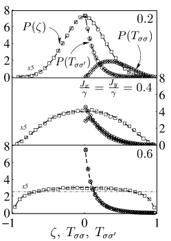
Figure 2: Distributions $P(\zeta)$, $P(T_{\sigma\sigma})$, and $P(T_{\sigma{\sigma}^{\prime}})$ for different spin-flip scattering strengths $J_{x}=J_{y}$ in the case of $N=10$. The dash-dotted line in the lowest panel indicates the uniform limit $P(\zeta)=1/2$ [note the magnification of $P(\zeta)$ by of factor of $5$] attained for strong enough spin-flip scattering.

IV Results and discussions

Figure 2 shows the distributions $P(\zeta)$, $P(T_{\sigma\sigma})$, and $P(T_{\sigma\sigma^{\prime}})$ for $N=10$ and increasing strengths of the spin-flip coupling $J_{x}=J_{y}$. The distribution $P(\zeta)$ is symmetric around $\zeta=0$ which implies that on average there is no spin filtering, $\langle\zeta\rangle$ $=0$. The distribution $P(\zeta)$ first gets narrower for spin flip in the $[0,0.15\gamma]$ range (not shown) and then broadens as spin flip further increases. For sufficiently strong spin-flip scattering the distribution approaches that of the uniform limit in which $P(\zeta)=1/2$. In this limit $P(T_{\sigma\sigma})$ and $P(T_{\sigma\sigma^{\prime}})$ coincide and so do all average transmission probabilities $\langle{T}_{\sigma\sigma^{\prime}}\rangle.$ As we discuss below, the initial narrowing and subsequent broadening of $P(\zeta)$ with spin flip gives rise to a minimum in the fluctuation of $\zeta$, Fig. 3.

Universal spin-polarization fluctuations. In the limit of a short spin-flip length $\ell_{\sigma}\ll L$ we in general find a uniform distribution $P(\zeta)=1/2$, Fig. 2. This uniform distribution yields the universal value $\langle(\delta\zeta)^{2}\rangle=1/3$ for the spin-polarization fluctuations. Figure 3 clearly shows that this universal value is attained for increasing spin flip strengths and is indeed independent of $N$. Interestingly, Fig. 3 also shows a minimum at around $J_{x}=J_{y}=0.15\gamma$. This minimum can be attributed to two competing energy scales: the longitudinal $(\sim J_{z})$ and the transverse $(\sim J_{x},J_{y})$ parts of the s-d exchange interaction, Eqs. (3) and (4), respectively. A simple “back-of-the-envelope” calculation shows that these two competing scales are equal for $J_{x}=J_{y}=J_{z}/\sqrt{2s(s+1)/3}\gamma=0.208\gamma$. The vertical dashed line in Fig. 3 indicates this value. Observe that $\langle(\delta\zeta)^{2}\rangle$ becomes larger for increasing $N$. This happens because $P(\zeta)$ broadens for larger $N$’s (the traversing electrons see a wider region with random spins). This is similar to the broadening due to increasing spin flip strength.

We should mention that the distribution $P(\zeta)$, and consequently $\langle(\delta\zeta)^{2}\rangle$, change dramatically for $\varepsilon_{F}<J_{z}$. In this regime, $P(\zeta)$ becomes U-shaped (not shown) because of the dominant filtering due to the “end states” with $S_{j,z}=\pm 5/2$. This qualitatively different $P(\zeta)$ yields a monotonically decreasing $\langle(\delta\zeta)^{2}\rangle$ as a function of spin-flip strength. Here the universal $\langle(\delta\zeta)^{2}\rangle=1/3$ value is approached from above for large spin flip strengths ($J_{x}=J_{y}\sim\gamma$).

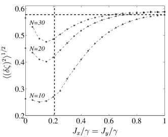
Figure 3: Average fluctuations $\big{<}(\delta\zeta)^{2}\big{>}^{1/2}$ as a function of spin-flip strength for $N=10$, $20$, and $30$. The dashed horizontal line indicates the universal value $1/\sqrt{3}$ obtained from the uniform limit $P(\zeta)=1/2$. The vertical dashed line indicates where the spin-flip rate is comparable to $|J_{z}\sigma|/\hbar$.

Suppression of conductance fluctuations. Whereas the fluctuations in the spin polarization $\zeta$ remain finite in the strong spin-flip scattering regime (Fig. 3), we find that the fluctuations of the conductance $g$ are strongly suppressed in this limit. This is illustrated in Fig. 4 which shows the average conductance and its fluctuations as a function of spin-flip scattering for $N=10$, $20$, and $30$. Note that $\langle(\delta g)^{2}\rangle^{1/2}$ is much more sensitive to spin flip than $\langle g\rangle$. In addition, for all $N$ we essentially have $\langle(\delta g)^{2}\rangle^{1/2}>\langle g\rangle$ for $J_{x}=J_{y}\rightarrow 0$ and $\langle(\delta g)^{2}\rangle^{1/2}\lesssim\langle g\rangle$ for $J_{x}=J_{y}\rightarrow\gamma$. Figure 4 clearly shows the conductance fluctuations get suppressed for increasing $N$. The horizontal dashed line shows the UCF value ($0.73/2=0.365$, see e.g. Ref. UCF, ) for a 1D wire in the metallic regime. The spin-related conductance fluctuations do not approach a finite value for increasing spin flip scattering. It actually seems to go to zero. This is in contrast to the spin-polarization fluctuations, Fig. 3, which attain a universal value $\langle(\delta\xi)^{2}\rangle^{1/2}=1/\sqrt{3}$ for strong spin-flip scattering. Incidentally, we observe that $\langle(\delta g)^{2}\rangle^{1/2}$ and $\langle(\delta\zeta)^{2}\rangle^{1/2}$ also present contrasting behavior for increasing $N$ (and $\varepsilon_{F}>J_{z}$): the former gets suppressed while the latter gets enhanced (cf. Figs. 3 and 4).

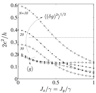
Figure 4: Average conductance $\langle g\rangle$ and its fluctuations $\big{<}(\delta g)^{2}\big{>}^{1/2}$ as a function of the spin-flip scattering strength for $N=10$, $20$, and $30$. The conductance fluctuations are much more sensitive to spin flip than the average conductance: the former gets strongly suppressed for increasing spin flip rates.

Spin disorder as spatial disorder. To some extent, the s-d site interaction considered here plays the role of spatial disorder in the system with a mean-free path $\ell_{J}$. Let us consider first the case with no spin flip (i.e., $J_{x}=J_{y}=0$). In this case, the term $J_{z}\sigma S_{n,z}$ acts as a “random” spin-dependent potential along the chain (here the site potential has some internal structure). As shown in Fig. 4 the conductance fluctuations for zero spin-flip scattering are larger than, slightly above, and slightly below, the UCF value for $N=10$, $N=20$, and $N=30$, respectively. For increasing $N$ we go from the metallic regime ($L=Na\ll\ell_{J_{z}}$) with vanishing fluctuations and a Gaussian $P(g)$ strongly peaked near $g\sim 2e^{2}/h$ to the strongly localized regime ($L\gg\ell_{J_{z}}$) where it is well-known that $P(g)$ is strongly peaked near $g\sim 0$ with a log-normal distribution so that fluctuations can be comparable to the mean value.beenakker1997 This is in accordance with numerical studies with different continuous distributions of the “on-site” potential (e.g. Gaussian or uniform distributions).kramer1993 In Fig. 4 the “small” mean values $\langle g\rangle$, for $N=10,20$, and 30, indicate the onset of localization with fluctuations comparable to the mean value. As $N$ gets larger conductance fluctuations are as expected suppressed beenakker1997 ; mirlin2000 .

Role of spin-flip scattering. Spin flip clearly suppresses conductance fluctuations, Fig. 4. This can be understood from Eq. (4) being a complex number with a random phase which makes spin flip act as a source of “de-coherence” [the total wave function is, of course, fully coherent]. Furthermore, spin flip mixes all the $S_{n,z}$ components on each site thus smoothing the potential seen by the traversing electron and hence reducing conductance fluctuations. This is true for both $\varepsilon_{F}>J_{z}$ [except for the window $[0,0.15\gamma]$ in which $P(\zeta)$ narrows] and $\varepsilon_{F}<J_{z}$.

“Truly” universal fluctuations. Why is $\langle(\delta\zeta)^{2}\rangle^{1/2}$ universal even for short spin-flip lengths $\ell_{\sigma}\ll L$ (strong spin-flip scattering) while $\langle(\delta g)^{2}\rangle^{1/2}$ is clearly suppressed below the usual UCF value in this limit? It is well known that conductance fluctuations are suppressed in the incoherent limit. UCF More specifically, in 1D wires with $\ell_{\varphi}\ll L$, $\ell_{\varphi}$ is some “dephasing length”, the suppression factor is $\sqrt{L/\ell_{\varphi}}$ (see Ref. [datta, ]). Interestingly, we can likewise understand the suppression of $\langle(\delta g)^{2}\rangle^{1/2}$ seen in our simulations by viewing spin-flip scattering as producing “dephasing” with $\ell_{\varphi}\sim\ell_{J_{x,y}}$ dephasing . For the spin-polarization fluctuations, however, the picture is slightly different: here we divide our system in $N_{L}=L/l_{\varphi}$ segments. To each of these we can associate an average spin polarization $\langle\zeta_{i}\rangle=0$ $(i$: $1..N_{L})$  and a corresponding spin-polarization fluctuation $\langle(\delta\zeta_{i})^{2}\rangle$. Neither $\langle\zeta_{i}\rangle$ nor $\langle(\delta\zeta_{i})^{2}\rangle$ are additive quantities like $\langle g\rangle$ and $\langle(\delta g)^{2}\rangle$ (“extensive versus intensive” properties). Sensible global averages for the whole system are then $\bar{\zeta}\equiv\frac{1}{N_{L}}\sum_{i}\langle\zeta_{i}\rangle=0$ and $\overline{{(\delta\zeta)}^{2}}\equiv\frac{1}{N_{L}}\sum_{i}\langle(\delta\zeta_{i})^{2}\rangle$. We should expect $\overline{{(\delta\zeta)}^{2}}=$ $\langle(\delta\zeta_{i})^{2}\rangle\equiv\langle(\delta\zeta)^{2}\rangle$ if the system is ergodic. Hence universal spin-polarization fluctuations are not suppressed for large spin-flip scattering in contrast to conductance fluctuations.

V Concluding remarks

Spin-flip scattering in Mn-based wires reduces conductance fluctuations while enhancing spin-polarization fluctuations in a limited parameter range. Remarkably, spin-polarization fluctuations reach a universal value $1/3$ for large spin-flip scattering in which the conductance fluctuations vanish. This universal value should manifest itself in time- and polarization-resolved photo-luminescence measurements. More important, these sizable spin fluctuations may limit the possibilities for steady spin injection in these systems.

The authors thank A.-P. Jauho for a critical reading of the manuscript. We also acknowledge K. Flensberg (NAM), U. Zülicke and M. Governale (JCE) for useful discussions. This work has been supported by the Swiss NSF, DARPA, ARO, and FAPESP/Brazil (JCE).

References

- (1) S. A. Wolf et al., Science 294, 1488 (2001).
- (2) J. M. Kikkawa and D. D. Awschalom, Nature 397, 139 (1999).
- (3) R. Fiederling et al., Nature 402, 787 (1999); Y. Ohno et al., ibid. 402, 790 (1999).
- (4) J. C. Egues, Phys. Rev. Lett 80, 4578 (1998); K. Chang and F. M. Peeters, Solid State Commun. 120, 181 (2001); Y. Guo et al., Phys. Rev. B 64, 155312 (2001).
- (5) P. Farinas, Phys. Rev. B 64, R161310 (2001).
- (6) F. G. Brito et al., J. Magn. Magn. Mater. 226, 457 (2001).
- (7) B. K. Nikolic and J. K. Freericks, cond-mat/0111144.
- (8) J. Jaroszyński et al., Phys. Rev. Lett. 75, 3170 (1995).
- (9) O. Ray et al., Appl. Phys. Lett. 76, 1167 (2000); H. Ikada et al., Physica E 10, 373 (2001).
- (10) J. K. Furdyna, J. App. Phys. 64, R29 (1988).
- (11) R. Landauer, IBM J. Res. Dev. 1, 223 (1957); Philos. Mag. 21, 863 (1970).
- (12) S. Datta, Electronic Transport in Mesoscopic Systems (Cambridge University Press, Cambridge, 1995).
- (13) For “intermediate” spin-flip scattering strengths (see Fig. 4) we find the usual UCF value for the conductance fluctuations. In this parameter range, our numerical calculation seems to be consistent with the experimental results of Ref. [dietl, ] in which no s-d induced effects were observed on the mean amplitude of the UCF.
- (14) D. S. Fisher and P. A. Lee, Phys. Rev. B 23, 6851 (1981).
- (15) C. W. J. Beenakker and H. van Houten, in Solid State Physics, edited by H. Ehrenreich and D. Turnbull (Academic Press, New York, 1991), Vol. 44, pp. 1–228.
- (16) C. W. J. Beenakker, Rev. Mod. Phys. 69, 731 (1997).
- (17) B. Kramer and A. MacKinnon, Rep. Prog. Phys. 56, 1469 (1993).
- (18) A. D. Mirlin, Phys. Rep. 326, 259 (2000).
- (19) Again, this is a sensible view since spin flip is a complex number with a random phase in our model, see Eq. (4).