The LDA+DMFT Approach to Materials with Strong Electronic Correlations

Abstract

LDA+DMFT is a novel computational technique for ab initio investigations of real materials with strongly correlated electrons, such as transition metals and their oxides. It combines the strength of conventional band structure theory in the local density approximation (LDA) with a modern many-body approach, the dynamical mean-field theory (DMFT). In the last few years LDA+DMFT has proved to be a powerful tool for the realistic modeling of strongly correlated electronic systems. In this paper the basic ideas and the set-up of the LDA+DMFT(X) approach, where X is the method used to solve the DMFT equations, are discussed. Results obtained with X=QMC (quantum Monte Carlo) and X=NCA (non-crossing approximation) are presented and compared. By means of the model system La_1-xSr_xTiO₃ we show that the method X matters qualitatively and quantitatively. Furthermore, we discuss recent results on the Mott-Hubbard metal-insulator transition in the transition metal oxide V₂O₃ and the $\alpha$-$\gamma$ transition in the 4f-electron system Ce.

Table of contents

1.	Introduction	1
2.	The LDA+DMFT approach	2
	2.1.  Density functional theory	2.1
	2.2.  Local density approximation	2.2
	2.3.  Supplementing LDA with local Coulomb correlations	2.3
	2.4.  Dynamical mean-field theory	2.4
	2.5.  QMC method to solve DMFT	2.5
	2.6.  NCA method to solve DMFT	2.6
	2.7.  Simplifications for transition metal oxides with well separated $e_{g}$- and $t_{2g}$-bands	2.7
	2.8.  Self-consistent LDA+DMFT	2.8
3.	Comparison of different methods to solve DMFT	3
4.	Mott-Hubbard metal-insulator transition in V2O3	4
5.	The Cerium volume collapse	5
6.	Conclusion and Outlook	6

To be published in the Proceedings of the Winter School on ”Quantum Simulations of Complex Many-Body Systems: From Theory to Algorithms”, February 25 - March 1, 2002, Rolduc/Kerkrade (NL), organized by the John von Neumann Institute of Computing at the Forschungszentrum Jülich.

1 Introduction

The calculation of physical properties of electronic systems by controlled approximations is one of the most important challenges of modern theoretical solid state physics. In particular, the physics of transition metal oxides – a singularly important group of materials both from the point of view of fundamental research and technological applications – may only be understood by explicit consideration of the strong effective interaction between the conduction electrons in these systems. The investigation of electronic many-particle systems is made especially complicated by quantum statistics, and by the fact that the investigation of many phenomena require the application of non-perturbative theoretical techniques.

From a microscopic point of view theoretical solid state physics is concerned with the investigation of interacting many-particle systems involving electrons and ions. However, it is an established fact that many electronic properties of matter are well described by the purely electronic Hamiltonian

$$\hat{H} = \sum_{\sigma}\int\!d^{3}r\;\hat{\Psi}^{+}({\bf r},\sigma)\left[{-\frac{\hbar^{2}}{2m_{e}}\Delta+V_{{\rm ion}}({\bf r})}\right]\hat{\Psi}({\bf r},\sigma)$$ (1)

$$+\frac{1}{2}\sum_{\sigma\sigma^{\prime}}\int\!d^{3}r\,d^{3}r^{\prime}\;\hat{\Psi}^{+}({\bf r},\sigma)\hat{\Psi}^{+}({\bf r^{\prime}},\sigma^{\prime})\;{V_{{\rm ee}}({\bf r}\!-\!{\bf r^{\prime}})}\;\hat{\Psi}({\bf r^{\prime}},\sigma^{\prime})\hat{\Psi}({\bf r},\sigma),$$

where the crystal lattice enters only through an ionic potential. The applicability of this approach may be justified by the validity of the Born and Oppenheimer approximation[1]. Here, $\hat{\Psi}^{+}({\bf r},\sigma)$ and $\hat{\Psi}({\bf r},\sigma)$ are field operators that create and annihilate an electron at position ${\bf r}$ with spin $\sigma$, $\Delta$ is the Laplace operator, $m_{e}$ the electron mass, $e$ the electron charge, and

$$V_{{\rm ion}}({\bf r})=-e^{2}\sum_{i}\frac{Z_{i}}{|{\bf r}-{\bf R_{i}}|} \;\;{\rm and}\;\; V_{\rm ee}({\bf r}\!-\!{\bf r^{\prime}})=\frac{e^{2}}{2}\sum_{{\bf r}\neq{\bf r^{\prime}}}\frac{1}{|{\bf r}-{\bf r^{\prime}}|}$$ (2)

denote the one-particle potential due to all ions $i$ with charge $eZ_{i}$ at given positions ${\bf R_{i}}$, and the electron-electron interaction, respectively.

While the ab initio Hamiltonian (1) is easy to write down it is impossible to solve exactly if more than a few electrons are involved. Numerical methods like Green’s Function Monte Carlo and related approaches have been used successfully for relatively modest numbers of electrons. Even so, however, the focus of the work has been on jellium and on light atoms and molecules like H, H₂, ³He, ⁴He, see, e.g., the articles by Anderson, Bernu, Ceperley et al. in the present Proceedings of the NIC Winterschool 2002. Because of this, one generally either needs to make substantial approximations to deal with the Hamiltonian (1), or replace it by a greatly simplified model Hamiltonian. At present these two different strategies for the investigation of the electronic properties of solids are applied by two largely separate groups: the density functional theory (DFT) and the many-body community. It is known for a long time already that DFT, together with its local density approximation (LDA), is a highly successful technique for the calculation of the electronic structure of many real materials[2]. However, for strongly correlated materials, i.e., $d$- and $f$-electron systems which have a Coulomb interaction comparable to the band-width, DFT/LDA is seriously restricted in its accuracy and reliability. Here, the model Hamiltonian approach is more general and powerful since there exist systematic theoretical techniques to investigate the many-electron problem with increasing accuracy. These many-body techniques allow one to describe qualitative tendencies and understand the basic mechanism of various physical phenomena. At the same time the model Hamiltonian approach is seriously restricted in its ability to make quantitative predictions since the input parameters are not accurately known and hence need to be adjusted. One of the most successful techniques in this respect is the dynamical mean-field theory (DMFT) – a non-perturbative approach to strongly correlated electron systems which was developed during the past decade[3, 4, 5, 6, 7, 8, 9, 10, 11]. The LDA+DMFT approach, which was first formulated by Anisimov et al.[12, 13], combines the strength of DFT/LDA to describe the weakly correlated part of the ab initio Hamiltonian (1), i.e., electrons in $s$- and $p$-orbitals as well as the long-range interaction of the $d$- and $f$-electrons, with the power of DMFT to describe the strong correlations induced by the local Coulomb interaction of the $d$- or $f$-electrons.

Starting from the ab initio Hamiltonian (1), the LDA+DMFT approach is presented in Section 2, including the DFT in Section 2.1, the LDA in Section 2.2, the construction of a model Hamiltonian in Section 2.3, and the DMFT in Section 2.4. As methods used to solve the DMFT we discuss the quantum Monte Carlo (QMC) algorithm in Section 2.5 and the non-crossing approximation (NCA) in Section 2.6. A simplified treatment for transition metal oxides is introduced in Section 2.7, and the scheme of a self-consistent LDA+DMFT in Section 2.8. As a particular example, the LDA+DMFT calculation for La_1-xSr_xTiO₃ is discussed in Section 3, emphasizing that the method X to solve the DMFT matters on a quantitative level. Our calculations for the Mott-Hubbard metal-insulator transition in V₂O₃ are presented in Section 4, in comparison to the experiment. Section 5 reviews our recent calculations of the Ce $\alpha$-$\gamma$ transition, in the perspective of the models referred to as Kondo volume collapse and Mott transition scenario. A discussion of the LDA+DMFT approach and its future prospects in Section 6 closes the presentation.

2 The LDA+DMFT approach

2.1 Density functional theory

The fundamental theorem of DFT by Hohenberg and Kohn[14] (see, e.g., the review by Jones and Gunnarsson[2]) states that the ground state energy is a functional of the electron density which assumes its minimum at the ground state electron density. Following Levy,[15] this theorem is easily proved and the functional even constructed by taking the minimum (infimum) of the energy expectation value w.r.t. all (many-body) wave functions $\varphi({\bf r_{1}}\sigma_{1},...\,{\bf r_{N}}\sigma_{N})$ at a given electron number $N$ which yield the electron density $\rho({\bf r})$:

$$E[\rho]=\inf\Big{\{}\langle\varphi|\hat{H}|\varphi\rangle\;\;\Big{|}\;\;\langle\varphi|\sum_{i=1}^{N}\delta({\bf r}-{\bf r_{i}})|\varphi\rangle=\rho({\bf r})\Big{\}}.$$ (3)

However, this construction is of no practical value since it actually requires the evaluation of the Hamiltonian (1). Only certain contributions like the Hartree energy $E_{{\rm Hartree}}[\rho]=\frac{1}{2}\int d^{3}r^{\prime}\,d^{3}r\;V_{{\rm ee}}({\bf r}\!-\!{\bf r^{\prime}})\;\rho({\bf r^{\prime})\rho(r)}$ and the energy of the ionic potential $E_{{\rm ion}}[\rho]=\int d^{3}r\;V_{{\rm ion}}({\bf r})\;\rho({\bf r)}$ can be expressed directly in terms of the electron density. This leads to

$$E[\rho]=E_{{\rm kin}}[\rho]+E_{{\rm ion}}[\rho]+E_{{\rm Hartree}}[\rho]+E_{{\rm xc}}[\rho],$$ (4)

where $E_{{\rm kin}}[\rho]$ denotes the kinetic energy, and $E_{{\rm xc}}[\rho]$ is the unknown exchange and correlation term which contains the energy of the electron-electron interaction except for the Hartree term. Hence all the difficulties of the many-body problem have been transferred into $E_{{\rm xc}}[\rho]$. While the kinetic energy $E_{{\rm kin}}$ cannot be expressed explicitly in terms of the electron density one can employ a trick to determine it. Instead of minimizing $E[\rho]$ with respect to $\rho$ one minimizes it w.r.t. a set of one-particle wave functions $\varphi_{i}$ related to $\rho$ via

$$\rho({\bf r})=\sum_{i=1}^{N}|\varphi_{i}({\bf r})|^{2}.$$ (5)

To guarantee the normalization of $\varphi_{i}$, the Lagrange parameters $\varepsilon_{i}$ are introduced such that the variation $\delta\{E[\rho]+\varepsilon_{i}[1-\int d^{3}r|\varphi_{i}({\bf r})|^{2}]\}/\delta\varphi_{i}({\bf r})=0$ yields the Kohn-Sham[16] equations:

$$\left[-{\frac{\hbar^{2}}{2m_{e}}\Delta+V_{{\rm ion}}({\bf r})}+\int d^{3}{r^{\prime}}\,{V_{{\rm ee}}({\bf r}\!-\!{\bf r^{\prime}})}{\rho({\bf r^{\prime}})}+{{\frac{\delta{E_{{\rm xc}}[\rho]}}{\delta\rho({\bf r)}}}}\right]\varphi_{i}({\bf r})=\varepsilon_{i}\;\varphi_{i}({\bf r}).$$ (6)

These equations have the same form as a one-particle Schrödinger equation which, a posteriori, justifies to calculate the kinetic energy by means of the one-particle wave-function ansatz. The kinetic energy of a one-particle ansatz which has the ground state density is, then, given by $E_{{\rm kin}}[\rho_{{\rm min}}]=-\sum_{i=1}^{N}\langle\varphi_{i}|{\hbar^{2}\Delta}/{(2m_{e})}|\varphi_{i}\rangle$ if the $\varphi_{i}$ are the self-consistent (spin-degenerate) solutions of Eqs. (6) and (5) with lowest “energy” $\epsilon_{i}$. Note, however, that the one-particle potential of Eq. (6), i.e.,

$$V_{\rm eff}({\bf r})=V_{{\rm ion}}({\bf r})+\int d^{3}{r^{\prime}}{V_{{\rm ee}}({\bf r}\!-\!{\bf r^{\prime}})}{\rho({\bf r^{\prime}})}+{{\frac{\delta{E_{{\rm xc}}[\rho]}}{\delta\rho({\bf r)}}}},$$ (7)

is only an auxiliary potential which artificially arises in the approach to minimize $E[\rho]$. Thus, the wave functions $\varphi_{i}$ and the Lagrange parameters $\varepsilon_{i}$ have no physical meaning at this point. Altogether, these equations allow for the DFT/LDA calculation, see the flow diagram Fig. 1.

Figure 1: Flow diagram of the DFT/LDA calculations.

2.2 Local density approximation

So far no approximations have been employed since the difficulty of the many-body problem was only transferred to the unknown functional $E_{\rm xc}[\rho]$. For this term the local density approximation (LDA) which approximates the functional $E_{\rm xc}[\rho]$ by a function that depends on the local density only, i.e.,

$$E_{\rm xc}[\rho]\;{\rightarrow}\;\int d^{3}r\;E_{\rm xc}^{{\rm LDA}}(\rho({\bf r})),$$ (8)

was found to be unexpectedly successful. Here, $E_{\rm xc}^{{\rm LDA}}(\rho({\bf r}))$ is usually calculated from the perturbative solution[17] or the numerical simulation[18] of the jellium problem which is defined by $V_{{\rm ion}}({\bf r})={\rm const}$.

In principle DFT/LDA only allows one to calculate static properties like the ground state energy or its derivatives. However, one of the major applications of LDA is the calculation of band structures. To this end, the Lagrange parameters $\varepsilon_{i}$ are interpreted as the physical (one-particle) energies of the system under consideration. Since the true ground-state is not a simple one-particle wave-function, this is an approximation beyond DFT. Actually, this approximation corresponds to the replacement of the Hamiltonian (1) by

$$\hat{H}_{{\rm LDA}} = \sum_{\sigma}\int\!d^{3}r\;\hat{\Psi}^{+}({\bf r},\sigma)\left[-\frac{\hbar^{2}}{2m_{e}}\Delta+V_{{\rm ion}}({\bf r})+\int d^{3}{r^{\prime}}\,{\rho({\bf r^{\prime}})}{V_{{\rm ee}}({\bf r}\!-\!{\bf r^{\prime}})}\right.$$ (9)

$$\left.\phantom{\sum_{\sigma\sigma^{\prime}}\int\!d^{3}r\;\hat{\Psi}^{+}({\bf r},\sigma)\big{[}\;}+{{\frac{\delta{E_{\rm xc}^{{\rm LDA}}}[\rho]}{\delta\rho({\bf r)}}}}\right]\hat{\Psi}({\bf r},\sigma).$$

For practical calculations one needs to expand the field operators w.r.t. a basis $\Phi_{ilm}$, e.g., a linearized muffin-tin orbital (LMTO)[19] basis ($i$ denotes lattice sites; $l$ and $m$ are orbital indices). In this basis,

$$\hat{\Psi}^{+}({\bf r},\sigma) = \sum_{ilm}\hat{c}_{ilm}^{\sigma\dagger}\Phi_{ilm}({\bf r})^{\phantom{+}}$$ (10)

such that the Hamiltonian (9) reads

$$\hat{H}_{\rm LDA} = \sum_{ilm,{\rm}jl^{\prime}m^{\prime},\sigma}(\delta_{ilm,jl^{\prime}m^{\prime}}\;{\varepsilon_{ilm}}^{\phantom{\sigma}}{\hat{n}}_{ilm}^{\sigma}+{t_{ilm,jl^{\prime}m^{\prime}}}\;{\hat{c}}_{ilm}^{\sigma\dagger}{\hat{c}}_{jl^{\prime}m^{\prime}}^{\sigma}).$$ (11)

Here, ${\hat{n}}_{ilm}^{\sigma}=\hat{c}_{ilm}^{\sigma\dagger}{\hat{c}}_{ilm}^{\sigma}$,

$$t_{ilm,jl^{\prime}m^{\prime}}=\Big{\langle}\Phi_{ilm}\Big{|}-\frac{\hbar^{2}\Delta}{2m_{e}}+V_{{\rm ion}}({\bf r})+\int d^{3}{r^{\prime}}{\rho({\bf r^{\prime}})}{V_{{\rm ee}}({\bf r}\!-\!{\bf r^{\prime}})}+{{\frac{\delta{E_{\rm xc}^{{\rm LDA}}}[\rho]}{\delta\rho({\bf r)}}}}\Big{|}\Phi_{jl^{\prime}m^{\prime}}\Big{\rangle}$$ (12)

for $ilm\neq jl^{\prime}m^{\prime}$ and zero otherwise; $\varepsilon_{ilm}$ denotes the corresponding diagonal part.

As for static properties, the LDA approach based on the self-consistent solution of Hamiltonian (11) together with the calculation of the electronic density Eq. (5) [see the flow diagram Fig. 1] has also been highly successful for band structure calculations – but only for weakly correlated materials[2]. It is not reliable when applied to correlated materials and can even be completely wrong because it treats electronic correlations only very rudimentarily. For example, it predicts the antiferromagnetic insulator La₂CuO₄ to be a non-magnetic metal[20] and also completely fails to account for the high effective masses observed in $4f$-based heavy fermion compounds.

2.3 Supplementing LDA with local Coulomb correlations

Of prime importance for correlated materials are the local Coulomb interactions between $d$- and $f$-electrons on the same lattice site since these contributions are largest. This is due to the extensive overlap (w.r.t. the Coulomb interaction) of these localized orbitals which results in strong correlations. Moreover, the largest non-local contribution is the nearest-neighbor density-density interaction which, to leading order in the number of nearest-neighbor sites, yields only the Hartree term (see Ref. 4 and, also, Ref. 21) which is already taken into account in the LDA. To take the local Coulomb interactions into account, one can supplement the LDA Hamiltonian (11) with the local Coulomb matrix approximated by the (most important) matrix elements $U_{mm^{\prime}}^{\sigma\sigma^{\prime}}$ (Coulomb repulsion and Z-component of Hund’s rule coupling) and ${J_{mm^{\prime}}}$ (spin-flip terms of Hund’s rule coupling) between the localized electrons (for which we assume $i=i_{d}$ and $l=l_{d}$):

$$\hat{H} = \hat{H}_{\rm LDA}-\hat{H}_{\rm LDA}^{U}+\frac{1}{2}{\sum_{i=i_{d},l=l_{d}}\sum_{m\sigma,m^{\prime}\sigma^{\prime}}}^{\!\!\!\!\!\prime}\;\;{U_{mm^{\prime}}^{\sigma\sigma^{\prime}}}\hat{n}_{ilm\sigma}\hat{n}_{ilm^{\prime}\sigma^{\prime}}$$ (13)

$$-\frac{1}{2}{\sum_{i=i_{d},l=l_{d}}}\sum_{m\sigma,m^{\prime}}^{\;\;\;\;\;\;\;\;\;\prime}{J_{mm^{\prime}}}\hat{c}^{\dagger}_{ilm\sigma}\hat{c}^{\dagger}_{ilm^{\prime}\bar{\sigma}}\hat{c}^{\phantom{\dagger}}_{ilm^{\prime}\sigma}\hat{c}^{\phantom{\dagger}}_{ilm\bar{\sigma}}.$$

Here, the prime on the sum indicates that at least two of the indices of an operator have to be different, and $\bar{\sigma}=\downarrow\!(\uparrow)$ for $\sigma=\uparrow\!(\downarrow)$. A term $\hat{H}_{{\rm LDA}}^{U}$ is subtracted to avoid double-counting of those contributions of the local Coulomb interaction already contained in $\hat{H}_{{\rm LDA}}$. Since there does not exist a direct microscopic or diagrammatic link between the model Hamiltonian approach and LDA it is not possible to express $\hat{H}_{{\rm LDA}}^{U}$ rigorously in terms of $U$, $J$ and $\rho$. A commonly employed approximation for $\hat{H}_{{\rm LDA}}^{U}$ assumes the LDA energy $E_{\rm LDA}^{U}$ of $\hat{H}_{{\rm LDA}}^{U}$ to be[22]

$$E_{\rm LDA}^{U}=\frac{1}{2}\bar{U}n_{d}(n_{d}-1)-\frac{1}{2}{J}\sum_{\sigma}n_{d\sigma}(n_{d\bar{\sigma}}-1).$$ (14)

Here, $n_{d\sigma}=\sum_{m}n_{il_{d}m\sigma}=\sum_{m}\langle\hat{n}_{il_{d}m\sigma}\rangle$ is the total number of interacting electrons per spin, $n_{d}=\sum_{\sigma}n_{d\sigma}$, $\bar{U}$ is the average Coulomb repulsion and ${J}$ the average exchange or Hund’s rule coupling. In typical applications we have $U_{mm}^{\uparrow\downarrow}\equiv U$, $J_{mm^{\prime}}\equiv{J}$, $U_{mm^{\prime}}^{\sigma\sigma^{\prime}}=U-J-J\delta_{\sigma\sigma^{\prime}}$ for $m\neq m^{\prime}$ (here, the first term $J$ is due to the reduced Coulomb repulsion between different orbitals and the second term $J\delta_{\sigma\sigma^{\prime}}$ directly arises from the Z-component of Hund’s rule coupling), and (with the number of interacing orbitals $M$)

$$\bar{U}=\frac{U+(M-1)(U-J)+(M-1)(U-2J)}{2M-1}.$$

Since the one-electron LDA energies can be obtained from the derivatives of the total energy w.r.t. the occupation numbers of the corresponding states, the one-electron energy level for the non-interacting, paramagnetic states of (13) is obtained as[22]

$$\varepsilon_{il_{d}m}^{0}\equiv\frac{{\rm d}}{{\rm d}n_{il_{d}m}}(E_{{\rm LDA}}-E_{{\rm LDA}}^{U})=\varepsilon_{il_{d}m}-\bar{U}(n_{d}-\frac{1}{2})+\frac{{J}}{2}(n_{d}-1)$$ (15)

where $\varepsilon_{il_{d}m}$ is defined in (11) and $E_{{\rm LDA}}$ is the total energy calculated from $\hat{H}_{{\rm LDA}}$ (11). Furthermore we used $n_{d\sigma}=n_{d}/2$ in the paramagnet.

This leads to a new Hamiltonian describing the non-interacting system

$$\hat{H}^{0}_{{\rm LDA}} = \sum_{ilm,jl^{\prime}m^{\prime},\sigma}\!\!\!(\delta_{ilm,jl^{\prime}m^{\prime}}\varepsilon_{ilm}^{0}{\hat{n}}_{ilm}^{\sigma}+t_{ilm,jl^{\prime}m^{\prime}}{\hat{c}}_{ilm}^{\sigma\dagger}{\hat{c}}_{jl^{\prime}m^{\prime}}^{\sigma}),$$ (16)

where $\varepsilon_{il_{d}m}^{0}$ is given by (15) for the interacting orbitals and $\varepsilon_{ilm}^{0}=\varepsilon_{ilm}$ for the non-interacting orbitals. While it is not clear at present how to systematically subtract $\hat{H}_{{\rm LDA}}^{U}$ one should note that the subtraction of a Hartree-type energy does not substantially affect the overall behavior of a strongly correlated paramagnetic metal in the vicinity of a Mott-Hubbard metal-insulator transition (see also Section 2.7).

In the following, it is convenient to work in reciprocal space where the matrix elements of $\hat{H}_{{\rm LDA}}^{0}$, i.e., the LDA one-particle energies without the local Coulomb interaction, are given by

$$(H^{0}_{{\rm LDA}}({\bf k}))_{qlm,q^{\prime}l^{\prime}m^{\prime}}\! \ =\ \!(H_{{\rm LDA}}({\bf k}))_{qlm,q^{\prime}l^{\prime}m^{\prime}}$$ (17)

$$-\delta_{qlm,q^{\prime}l^{\prime}m^{\prime}}\delta_{ql,q_{d}l_{d}}\left[\bar{U}(n_{d}-\frac{1}{2})-\frac{J}{2}(n_{d}-1)\right].$$

Here, $q$ is an index of the atom in the elementary unit cell, $(H_{{\rm LDA}}({\bf k}))_{qlm,q^{\prime}l^{\prime}m^{\prime}}$ is the matrix element of (11) in ${\bf k}$-space, and $q_{d}$ denotes the atoms with interacting orbitals in the unit cell. The non-interacting part, $\hat{H}_{{\rm LDA}}^{0}$, supplemented with the local Coulomb interaction forms the (approximated) ab initio Hamiltonian for a particular material under investigation:

$$\hat{H} = \hat{H}_{{\rm LDA}}^{0}+\frac{1}{2}{\sum_{i=i_{d},l=l_{d}}\sum_{m\sigma,m^{\prime}\sigma^{\prime}}}^{\!\!\!\!\!\!\prime}\;\;\;{U_{mm^{\prime}}^{\sigma\sigma^{\prime}}}\hat{n}_{ilm\sigma}\hat{n}_{ilm^{\prime}\sigma^{\prime}}$$ (18)

$$-\frac{1}{2}{\sum_{i=i_{d},l=l_{d}}\sum_{m\sigma,m^{\prime}}}^{\!\!\!\prime}\;\;\;{J_{mm^{\prime}}}\hat{c}^{\dagger}_{ilm\sigma}\hat{c}^{\dagger}_{ilm^{\prime}\bar{\sigma}}\hat{c}^{\phantom{\dagger}}_{ilm^{\prime}\sigma}\hat{c}^{\phantom{\dagger}}_{ilm\bar{\sigma}}$$

To make use of this ab initio Hamiltonian it is still necessary to determine the Coulomb interaction $U$. To this end, one can calculate the LDA ground state energy for different numbers of interacting electrons $n_{d}$ (”constrained LDA”[23]) and employ Eq. (14) whose second derivative w.r.t. $n_{d}$ yields $U$. However, one should keep in mind that, while the total LDA spectrum is rather insensitive to the choice of the basis, the calculation of $U$ strongly depends on the shape of the orbitals which are considered to be interacting. E.g., for LaTiO₃ at a Wigner Seitz radius of 2.37 a.u. for Ti a LMTO-ASA calculation[24] using the TB-LMTO-ASA code[19] yielded $U=4.2$ eV in comparison to the value $U=3.2$ eV calculated by ASA-LMTO within orthogonal representation [25]. Thus, an appropriate basis like LMTO is mandatory and, even so, a significant uncertainty in $U$ remains.

2.4 Dynamical mean-field theory

The many-body extension of LDA, Eq. (18), was proposed by Anisimov et al.[22] in the context of their LDA+U approach. Within LDA+U the Coulomb interactions of (18) are treated within the Hartree-Fock approximation. Hence, LDA+U does not contain true many-body physics. While this approach is successful in describing long-range ordered, insulating states of correlated electronic systems it fails to describe strongly correlated paramagnetic states. To go beyond LDA+U and capture the many-body nature of the electron-electron interaction, i.e., the frequency dependence of the self-energy, various approximation schemes have been proposed and applied recently[12, 26, 27, 28, 29, 30]. One of the most promising approaches, first implemented by Anisimov et al.[12], is to solve (18) within DMFT[3, 4, 5, 6, 7, 8, 9, 10, 11] (”LDA+DMFT”). Of all extensions of LDA only the LDA+DMFT approach is presently able to describe the physics of strongly correlated, paramagnetic metals with well-developed upper and lower Hubbard bands and a narrow quasiparticle peak at the Fermi level. This characteristic three-peak structure is a signature of the importance of many-body effects.[7, 8]

Figure 2: If the number of neighboring lattice sites goes to infinity, the central limit theorem holds and fluctuations from site-to-site can be neglected. This means that the influence of these neighboring sites can be replaced by a mean influence, the dynamical mean-field described by the self energy ${\Sigma}_{lm}^{\sigma}(\omega)$. This DMFT problem is equivalent to the self-consistent solution of the $\bf k$-integrated Dyson equation (21) and the multi-band Anderson impurity model Eq. (20).

During the last ten years, DMFT has proved to be a successful approach to investigate strongly correlated systems with local Coulomb interactions[11]. It becomes exact in the limit of high lattice coordination numbers[3, 4] and preserves the dynamics of local interactions. Hence, it represents a dynamical mean-field approximation. In this non-perturbative approach the lattice problem is mapped onto an effective single-site problem (see Fig. 2) which has to be determined self-consistently together with the ${\bf k}$-integrated Dyson equation connecting the self energy $\Sigma$ and the Green function $G$ at frequency $\omega$:

$$G_{qlm,q^{\prime}l^{\prime}m^{\prime}}(\omega)=\!\frac{1}{V_{B}}\int{{d^{3}}{k}}\! \left(\left[\;\omega 1+\mu 1-H_{{\rm LDA}}^{0}({\bf k})-\Sigma(\omega)\right]^{-1}\right)_{qlm,q^{\prime}l^{\prime}m^{\prime}}.$$ (19)

Here, $1$ is the unit matrix, $\mu$ the chemical potential, the matrix $H_{{\rm LDA}}^{0}({\bf k})$ is defined in (17), $\Sigma(\omega)$ denotes the self-energy matrix which is non-zero only between the interacting orbitals, $[...]^{-1}$ implies the inversion of the matrix with elements $n$ (=$qlm$), $n^{\prime}$(=$q^{\prime}l^{\prime}m^{\prime}$), and the integration extends over the Brillouin zone with volume $V_{B}$.

The DMFT single-site problem depends on ${\cal G}(\omega)^{-1}=G(\omega)^{-1}+\Sigma(\omega)$ and is equivalent[7, 8] to an Anderson impurity model (the history and the physics of this model is summarized by Anderson in Ref. 31) if its hybridization $\Delta(\omega)$ satisfies ${\cal G}^{-1}(\omega)=\omega-\int d\omega^{\prime}\Delta(\omega^{\prime})/(\omega-\omega^{\prime})$. The local one-particle Green function at a Matsubara frequency $i\omega_{\nu}=i(2\nu+1)\pi/\beta$ ($\beta$: inverse temperature), orbital index $m$ ($l=l_{d}$, $q=q_{d}$), and spin $\sigma$ is given by the following functional integral over Grassmann variables $\psi^{\phantom{\ast}}$ and $\psi^{\ast}$:

$$G_{\nu m}^{\sigma}=-\frac{1}{{\cal Z}}\int{\cal D}[\psi]{\cal D}[\psi^{\ast}]\psi_{\nu m}^{\sigma\phantom{\ast}}\psi_{\nu m}^{\sigma\ast}e^{{\cal A}[\psi,\psi^{\ast},{\cal G}^{-1}]}.$$ (20)

Here, ${\cal Z}=\int{\cal D}[\psi]{\cal D}[\psi^{\ast}]\psi_{\nu m}^{\sigma\phantom{\ast}}\psi_{\nu m}^{\sigma\ast}\exp({\cal A}[\psi,\psi^{\ast},{\cal G}^{-1}])$ is the partition function and the single-site action ${\cal A}$ has the form (the interaction part of ${\cal A}$ is in terms of the “imaginary time” $\tau$, i.e., the Fourier transform of $\omega_{\nu}$)

$${\cal A}[\psi,\psi^{\ast},{\cal G}^{-1}]=\sum_{\nu,\sigma,m}\psi_{\nu m}^{\sigma\ast}({\cal G}_{\nu m}^{\sigma})^{-1}\psi_{\nu m}^{\sigma{\phantom{\ast}}}$$ (21)

$$-\frac{1}{2}\!\!\!{\sum_{m\sigma,m\sigma^{\prime}}}^{\!\!\!\!\!{}^{\prime}}\;\;U_{mm^{\prime}}^{\sigma\sigma^{\prime}}\int\limits_{0}^{\beta}d\tau\,\psi_{m}^{\sigma\ast}(\tau)\psi_{m}^{\sigma\phantom{\ast}}(\tau)\psi_{m^{\prime}}^{\sigma^{\prime}\ast}(\tau)\psi_{m^{\prime}}^{\sigma^{\prime}\phantom{\ast}}(\tau)$$

$$+\frac{1}{2}{\sum_{m\sigma,m}}^{\!\!{}^{\prime}}\;\;J_{mm^{\prime}}\int\limits_{0}^{\beta}d\tau\,\psi_{m}^{\sigma\ast}(\tau)\psi_{m}^{\bar{\sigma}}(\tau)\psi_{m^{\prime}}^{\bar{\sigma}\ast}(\tau)\psi_{m^{\prime}}^{\sigma}(\tau)\;\;.$$

This single-site problem (20) has to be solved self-consistently together with the k-integrated Dyson equation (19) to obtain the DMFT solution of a given problem, see the flow diagram Fig. 3.

Figure 3: Flow diagram of the DMFT self-consistency cycle.

Due to the equivalence of the DMFT single-site problem and the Anderson impurity problem a variety of approximative techniques have been employed to solve the DMFT equations, such as the iterated perturbation theory (IPT)[7, 11] and the non-crossing approximation (NCA) [32, 33, 34], as well as numerical techniques like quantum Monte Carlo simulations (QMC)[35], exact diagonalization (ED)[36, 11], or numerical renormalization group (NRG)[37]. QMC and NCA will be discussed in more detail in Section 2.5 and 2.6, respectively. IPT is non-self-consistent second-order perturbation theory in $U$ for the Anderson impurity problem (20) at half-filling. It represents an ansatz that also yields the correct perturbational $U^{2}$-term and the correct atomic limit for the self-energy off half-filling[38], for further details see Refs. 38, 12, 26. ED directly diagonalizes the Anderson impurity problem at a limited number of lattice sites and orbitals. NRG first replaces the conduction band by a discrete set of states at $D\Lambda^{-n}$ ($D$: bandwidth; $n=0,...,{\cal N}_{s}$) and then diagonalizes this problem iteratively with increasing accuracy at low energies, i.e., with increasing ${\cal N}_{s}$. In principle, QMC and ED are exact methods, but they require an extrapolation, i.e., the discretization of the imaginary time $\Delta\tau\rightarrow 0$ (QMC) or the number of lattice sites of the respective impurity model $N_{s}\rightarrow\infty$ (ED), respectively.

In the context of LDA+DMFT we refer to the computational schemes to solve the DMFT equations discussed above as LDA+DMFT(X) where X=IPT[12], NCA[30], QMC[24] have been investigated in the case of La_1-xSr_xTiO₃. The same strategy was formulated by Lichtenstein and Katsnelson[26] as one of their LDA++ approaches. Lichtenstein and Katsnelson applied LDA+DMFT(IPT)[42], and were the first to use LDA+DMFT(QMC)[43], to investigate the spectral properties of iron. Recently, also V₂O₃[44], Ca_2-xSr_xRuO₄ [45, 46], Ni[47], Fe[47], Pu[48, 49], and Ce[50, 51] have been studied by LDA+DMFT. Realistic investigations of itinerant ferromagnets (e.g., Ni) have also recently become possible by combining density functional theory with multi-band Gutzwiller wave functions.[52]

2.5 QMC method to solve DMFT

The self-consistency cycle of the DMFT (Fig. 3) requires a method to solve for the dynamics of the single-site problem of DMFT, i.e., Eq. (20). The QMC algorithm by Hirsch and Fye[35] is a well established method to find a numerically exact solution for the Anderson impurity model and allows one to calculate the impurity Green function $G$ at a given ${\cal G}^{-1}$ as well as correlation functions. In essence, the QMC technique maps the interacting electron problem Eq. (20) onto a sum of non-interacting problems where the single particle moves in a fluctuating, time-dependent field and evaluates this sum by Monte Carlo sampling, see the flow diagram Fig. 5 for an overview. To this end, the imaginary time interval $[0,\beta]$ of the functional integral Eq. (20) is discretized into $\Lambda$ steps of size $\Delta\tau=\beta/\Lambda$, yielding support points $\tau_{l}=l\Delta\tau$ with $l=1\dots\Lambda$. Using this Trotter discretization, the integral $\int_{0}^{\beta}d\tau$ is transformed to the sum $\sum_{l=1}^{\Lambda}\Delta\tau$ and the exponential terms in Eq. (20) can be separated via the Trotter-Suzuki formula for operators $\hat{A}$ and $\hat{B}$[53]

$$e^{-\beta(\hat{A}+\hat{B})}=\prod_{l=1}^{\Lambda}e^{-\Delta\tau\hat{A}}e^{-\Delta\tau\hat{B}}+{\cal O}(\Delta\tau),$$ (22)

which is exact in the limit $\Delta\tau\rightarrow 0$. The single site action $\cal A$ of Eq. (21) can now be written in the discrete, imaginary time as

$${\cal A}[\psi,\psi^{*},{\cal G}^{-1}] = \Delta\tau^{2}\sum_{\sigma\,m\,l,l^{\prime}=0}^{\Lambda-1}{\psi_{ml}^{\sigma}}^{*}{{\cal G}_{m}^{\sigma}}^{-1}(l\Delta\tau-l^{\prime}\Delta\tau)\psi_{ml^{\prime}}^{\sigma}$$ (23)

$$-\frac{1}{2}\Delta\tau{\sum}_{m\sigma,m^{\prime}\sigma^{\prime}}^{{}^{\prime}}U_{mm^{\prime}}^{\sigma\sigma^{\prime}}\sum_{l=0}^{\Lambda-1}{\psi_{ml}^{\sigma}}^{*}{\psi_{ml}^{\sigma}}{\psi_{m^{\prime}l}^{\sigma^{\prime}}}^{*}{\psi_{m^{\prime}l}^{\sigma^{\prime}}},$$

where the first term was Fourier-transformed from Matsubara frequencies to imaginary time. In a second step, the $M(2M-1)$ interaction terms in the single site action $\cal A$ are decoupled by introducing a classical auxiliary field $s_{lmm^{\prime}}^{\sigma{\sigma^{\prime}}}$:

$$\exp\left\{\frac{\Delta\tau}{2}U_{mm^{\prime}}^{\sigma\sigma^{\prime}}({\psi_{ml}^{\sigma}}^{*}{\psi_{ml}^{\sigma}}-{\psi_{m^{\prime}l}^{\sigma^{\prime}}}^{*}{\psi_{m^{\prime}l}^{\sigma^{\prime}}})^{2}\right\}=\qquad\qquad$$

$$\hfill\frac{1}{2}\sum_{s_{lmm^{\prime}}^{\sigma{\sigma^{\prime}}}\,=\pm 1}\exp\left\{\Delta\tau\lambda_{lmm^{\prime}}^{\sigma{\sigma^{\prime}}}s_{lmm^{\prime}}^{\sigma{\sigma^{\prime}}}({\psi_{ml}^{\sigma}}^{*}{\psi_{ml}^{\sigma}}-{\psi_{m^{\prime}l}^{\sigma^{\prime}}}^{*}{\psi_{m^{\prime}l}^{\sigma^{\prime}}})\right\},$$ (24)

where $\cosh(\lambda_{lmm^{\prime}}^{\sigma{\sigma^{\prime}}})=\exp(\Delta\tau U_{mm^{\prime}}^{\sigma\sigma^{\prime}}/2)$ and $M$ is the number of interacting orbitals. This so-called discrete Hirsch-Fye-Hubbard-Stratonovich transformation can be applied to the Coulomb repulsion as well as the Z-component of Hund’s rule coupling.[54] It replaces the interacting system by a sum of $\Lambda M(2M-1)$ auxiliary fields $s_{lmm^{\prime}}^{\sigma{\sigma^{\prime}}}$. The functional integral can now be solved by a simple Gauss integration because the Fermion operators only enter quadratically, i.e., for a given configuration ${\bf s}=\{s_{lmm^{\prime}}^{\sigma{\sigma^{\prime}}}\}$ of the auxiliary fields the system is non-interacting. The quantum mechanical problem is then reduced to a matrix problem

$$G_{\tilde{m}l_{1}l_{2}}^{\tilde{\sigma}}=\frac{1}{\cal Z}\frac{1}{2}\sum_{l}\sum_{m^{\prime}\sigma^{\prime},m^{\prime\prime}\sigma^{\prime\prime}}^{\;\;\;\;\;\;\;\;\;\prime}\sum_{s_{lm^{\prime\prime}m^{\prime}}^{{\sigma^{\prime\prime}}{\sigma^{\prime}}}\,=\pm 1}\left[(M_{\tilde{m}}^{\tilde{\sigma}\mathbf{s}})^{-1}\right]_{l_{1}l_{2}}\prod_{m\sigma}\det\mathbf{M}_{m}^{\sigma\mathbf{s}}$$ (25)

with the partition function $\cal Z$, the matrix

$$\mathbf{M}_{\tilde{m}}^{\tilde{\sigma}\mathbf{s}}=\Delta\tau^{2}[{\mathbf{G}^{\sigma}_{m}}^{-1}+\Sigma_{m}^{\sigma}]e^{-\mathbf{\tilde{\lambda}}^{\sigma\mathbf{s}}_{m}}+\mathbf{1}-e^{-\mathbf{\tilde{\lambda}}^{\sigma\mathbf{s}}_{m}}$$ (26)

and the elements of the matrix $\mathbf{\tilde{\lambda}}^{\sigma\mathbf{s}}_{m}$

$$\tilde{\lambda}^{\sigma\mathbf{s}}_{mll^{\prime}}=-\delta_{ll^{\prime}}\sum_{m^{\prime}\sigma^{\prime}}\lambda_{mm^{\prime}}^{\sigma\sigma^{\prime}}\tilde{\sigma}_{mm^{\prime}}^{\sigma\sigma^{\prime}}s_{lmm^{\prime}}^{\sigma\sigma^{\prime}}.$$ (27)

Here $\tilde{\sigma}_{mm^{\prime}}^{\sigma\sigma^{\prime}}=2\Theta(\sigma^{\prime}-\sigma+\delta_{\sigma\sigma^{\prime}}[m^{\prime}-m]-1)$ changes sign if $(m\sigma)$ and $(m^{\prime}\sigma^{\prime})$ are exchanged. For more details, e.g., for a derivation of Eq. (26) for the matrix $\bf M$, see Refs. 35, 11.

Since the sum in Eq. (25) consists of $2^{\Lambda M(2M-1)}$ addends, a complete summation for large $\Lambda$ is computationally impossible. Therefore the Monte Carlo method, which is often an efficient way to calculate high-dimensional sums and integrals, is employed for importance sampling of Eq. (25). In this method, the integrand $F(x)$ is split up into a normalized probability distribution $P$ and the remaining term $O$:

$$\int dxF(x)=\int dx\,O(x)\,P(x)\equiv\langle O\rangle_{P}$$ (28)

with

$$\int dxP(x)=1\qquad\text{and}\qquad P(x)\geq 0.$$ (29)

In statistical physics, the Boltzmann distribution is often a good choice for the function $P$:

$$P(x)=\frac{1}{\cal Z}\exp(-\beta E(x)).$$ (30)

For the sum of Eq. (25), this probability distribution translates to

$$P(\mathbf{s})=\frac{1}{\cal Z}\prod_{m\sigma}\det\mathbf{M}_{m}^{\sigma\mathbf{s}}$$ (31)

with the remaining term

$$O(\mathbf{s})_{\tilde{m}l_{1}l_{2}}^{\tilde{\sigma}}=\left[(M_{\tilde{m}}^{\tilde{\sigma}\mathbf{s}})^{-1}\right]_{l_{1}l_{2}}.$$ (32)

Figure 4: Flow diagram of the QMC algorithm to calculate the Green function matrix ${\mathbf{G}}$ using the procedure MC-sweep of Fig. 5.

Figure 5: Procedure MC-sweep using the Metropolis[55] rule to change the sign of $s_{lmm^{\prime}}^{\sigma{\sigma^{\prime}}}$. The recalculation of ${\mathbf{G}}_{\rm cur}$, i.e., the matrix $\mathbf{M}$ of Eq. (26), simplifies to ${\cal O}(\Lambda^{2})$ operations if only one $s_{lmm^{\prime}}^{\sigma{\sigma^{\prime}}}$ changes sign.[35, 11]

Instead of summing over all possible configurations, the Monte Carlo simulation generates configurations $x_{i}$ with respect to the probability distribution $P(x)$ and averages the observable $O(x)$ over these $x_{i}$. Therefore the relevant parts of the phase space with a large Boltzmann weight are taken into account to a greater extent than the ones with a small weight, coining the name importance sampling for this method. With the central limit theorem one gets for $\cal N$ statistically independent addends the estimate

$$\langle O\rangle_{P}=\frac{1}{\cal N}\sum^{\cal N}_{\underset{x_{i}\in P(x)}{i=1}}O(x_{i})\pm\frac{1}{\sqrt{\cal N}}\sqrt{\langle O^{2}\rangle_{P}-\langle O\rangle_{P}^{2}}.$$ (33)

Here, the error and with it the number of needed addends $\cal N$ is nearly independent of the dimension of the integral. The computational effort for the Monte Carlo method is therefore only rising polynomially with the dimension of the integral and not exponentially as in a normal integration. Using a Markov process and single spin-flips in the auxiliary fields, the computational cost of the algorithm in leading order of $\Lambda$ is

$$2{a}M(2M-1)\Lambda^{3}\times\text{number of MC-sweeps},$$ (34)

where $a$ is the acceptance rate for a single spin-flip.

The advantage of the QMC method (for the algorithm see the flow diagram Fig. 5) is that it is (numerically) exact. It allows one to calculate the one-particle Green function as well as two-particle (or higher) Green functions. On present workstations the QMC approach is able to deal with up to seven interacting orbitals and temperatures above about room temperature. Very low temperatures are not accessible because the numerical effort grows like $\Lambda^{3}\propto 1/T^{3}$ . Since the QMC approach calculates $G(\tau)$ or $G(i\omega_{n})$ with a statistical error, it also requires the maximum entropy method[56] to obtain the Green function $G(\omega)$ at real (physical) frequencies $\omega$.

2.6 NCA method to solve DMFT

The NCA approach is a resolvent perturbation theory in the hybridization parameter $\Delta(\omega)$ of the effective Anderson impurity problem[32]. Thus, it is reliable if the Coulomb interaction $U$ is large compared to the band-width and also offers a computationally inexpensive approach to check the general spectral features in other situations.

To see how the NCA can be adapted for the DMFT, let us rewrite Eq. (19) as

$$G_{\sigma}(z)=\frac{1}{N_{k}}\sum_{{\bf k}}\big{[}{z-H_{LDA}^{0}({\bf k})-\Sigma(z)}\big{]}^{-1}$$ (35)

where $z=\omega+i0^{+}+\mu$. Again, $H_{LDA}^{0}({\bf k})$, $\Sigma(z)$ and hence $G^{0}_{\sigma}(\zeta)$ and $G_{\sigma}(z)$ are matrices in orbital space. Note that $\Sigma(z)$ has nonzero entries for the correlated orbitals only.

On quite general grounds, Eq. (35) can be cast into the form

$$G_{\sigma}(z)=\frac{1}{z-E^{0}-\Sigma_{\sigma}(z)-\Delta_{\sigma}(z)}$$ (36)

where

$$E^{0}=\frac{1}{N_{k}}\sum\limits_{\bf k}H_{LDA}^{0}({\bf k})$$ (37)

with the number of ${\bf k}$ points $N_{k}$ and

$$\lim_{\omega\rightarrow\pm\infty}\Re e\{\Delta_{\sigma}(\omega+i\delta)\}=0\;\;.$$ (38)

Given the the matrix $E^{0}$, the Coulomb matrix $U$ and the hybridization matrix $\Delta_{\sigma}(z)$, we are now in a position to set up a resolvent perturbation theory with respect to $\Delta_{\sigma}(z)$. To this end, we first have to diagonalize the local Hamiltonian

$$\begin{array}[]{l@{\,=\,}l}\displaystyle H_{\rm local}&\begin{array}[t]{l}\displaystyle\sum\limits_{\sigma}\sum\limits_{qml}\sum\limits_{q^{\prime}m^{\prime}l^{\prime}}c^{\dagger}_{qlm\sigma}E^{0}_{qlm,q^{\prime}l^{\prime}m^{\prime}}c^{\phantom{{}^{\dagger}}}_{qlm\sigma}\\[21.33955pt] \displaystyle+\frac{1}{2}\sum\limits_{m\sigma}\sum\limits_{m^{\prime}\sigma^{\prime}}U_{mm^{\prime}}^{\sigma\sigma^{\prime}}n_{q_{d}l_{d}m\sigma}n_{q_{d}l_{d}m^{\prime}\sigma^{\prime}}\\[21.33955pt] \displaystyle-\frac{1}{2}\sum\limits_{m\sigma}\sum\limits_{m^{\prime}}J_{mm^{\prime}}c^{\dagger}_{q_{d}l_{d}m\sigma}c^{\dagger}_{q_{d}l_{d}m^{\prime}\bar{\sigma}}c^{\phantom{\dagger}}_{q_{d}l_{d}m^{\prime}\sigma}c^{\phantom{\dagger}}_{q_{d}l_{d}m\bar{\sigma}}\\[21.33955pt] \end{array}\\ &\displaystyle\sum\limits_{\alpha}E_{\alpha}|\alpha\rangle\langle\alpha|\end{array}$$ (39)

with local eigenstates $|\alpha\rangle$ and energies $E_{\alpha}$. In contrast to the QMC, this approach allows one to take into account the full Coulomb matrix plus spin-orbit coupling.

With the states $|\alpha\rangle$ defined above, the fermionic operators with quantum numbers $\kappa=(q,l,m)$ are expressed as

$$\begin{array}[]{l@{\,=\,}l}\displaystyle c^{\dagger}_{\kappa\sigma}&\displaystyle\sum\limits_{\alpha,\beta}\left(D^{\kappa\sigma}_{\beta\alpha}\right)^{*}|\alpha\rangle\langle\beta|\>,\\[14.22636pt] \displaystyle c^{\phantom{dagger}}_{\kappa\sigma}&\displaystyle\sum\limits_{\alpha,\beta}D^{\kappa\sigma}_{\alpha\beta}|\alpha\rangle\langle\beta|\;\;.\end{array}$$ (40)

The key quantity for the resolvent perturbation theory is the resolvent $R(z)$, which obeys a Dyson equation [32]

$$R(z)=R^{0}(z)+R^{0}(z)S(z)R(z)\;\;,$$ (41)

where $R_{\alpha\beta}^{0}(z)=1/(z-E_{\alpha})\delta_{\alpha\beta}$ and $S_{\alpha\beta}(z)$ denotes the self-energy for the local states due to the coupling to the environment through $\Delta(z)$.

The self-energy $S_{\alpha\beta}(z)$ can be expressed as power series in the hybridization $\Delta(z)$ [32]. Retaining only the lowest-, i.e. $2^{nd}$-order terms leads to a set of self-consistent integral equations

$$\begin{array}[]{c}\displaystyle S_{\alpha\beta}(z)=\begin{array}[t]{l}\displaystyle\sum\limits_{\sigma}\sum\limits_{\kappa\kappa^{\prime}}\sum\limits_{\alpha^{\prime}\beta^{\prime}}\int\frac{d\varepsilon}{\pi}\,f(\varepsilon)\,\left(D^{\kappa\sigma}_{\alpha^{\prime}\alpha}\right)^{*}\Gamma^{\kappa\kappa^{\prime}}_{\sigma}(\varepsilon)R_{\alpha^{\prime}\beta^{\prime}}(z+\varepsilon)D^{\kappa^{\prime}\sigma}_{\beta^{\prime}\beta}\\[14.22636pt] \displaystyle+\sum\limits_{\sigma}\sum\limits_{\kappa\kappa^{\prime}}\sum\limits_{\alpha^{\prime}\beta^{\prime}}\int\frac{d\varepsilon}{\pi}\,(1-f(\varepsilon))\,D^{\kappa\sigma}_{\alpha^{\prime}\alpha}\Gamma^{\kappa\kappa^{\prime}}_{\sigma}(\varepsilon)R_{\alpha^{\prime}\beta^{\prime}}(z-\varepsilon)\left(D^{\kappa^{\prime}\sigma}_{\beta^{\prime}\beta}\right)^{*}\end{array}\end{array}$$ (42)

to determine $S_{\alpha\beta}(z)$, where $f(\varepsilon)$ denotes Fermi’s function and $\Gamma(\varepsilon)=-\Im m\left\{\Delta(\varepsilon+i0^{+})\right\}$. The set of equations (42) are in the literature referred to as non-crossing approximation (NCA), because, when viewed in terms of diagrams, they contain no crossing of band-electron lines. In order to close the cycle for the DMFT, we still have to calculate the true local Green function $G_{\sigma}(z)$. This, however, can be done within the same approximation with the result

$$G^{\kappa\kappa^{\prime}}_{\sigma}(i\omega)=\frac{1}{Z_{\rm local}}\sum\limits_{\alpha,\alpha^{\prime}}\sum\limits_{\nu,\nu^{\prime}}D^{\kappa\sigma}_{\alpha\alpha^{\prime}}\left(D^{\kappa^{\prime}\sigma}_{\nu\nu^{\prime}}\right)^{*}\oint\frac{dze^{-\beta z}}{2\pi i}R_{\alpha\nu}(z)R_{\alpha^{\prime}\nu^{\prime}}(z+i\omega)\;\;.$$ (43)

Here, $\displaystyle Z_{\rm local}=\sum\limits_{\alpha}\oint\frac{dze^{-\beta z}}{2\pi i}R_{\alpha\alpha}(z)$ denotes the local partition function and $\beta$ is the inverse temperature.

Like any other technique, the NCA has its merits and disadvantages. As a self-consistent resummation of diagrams it constitutes a conserving approximation to the Anderson impurity model. Furthermore, it is a (computationally) fast method to obtain dynamical results for this model and thus also within DMFT. However, the NCA is known to violate Fermi liquid properties at temperatures much lower than the smallest energy scale of the problem and whenever charge excitations become dominant[57, 34]. Hence, in some parameter ranges it fails in the most dramatic way and must therefore be applied with considerable care[34].

2.7 Simplifications for transition metal oxides with well separated $e_{g}$- and $t_{2g}$-bands

Many transition metal oxides are cubic perovskites, with only a slight distortion of the cubic crystal structure. In these systems the transition metal $d$-orbitals lead to strong Coulomb interactions between the electrons. The cubic crystal-field of the oxygen causes the $d$-orbitals to split into three degenerate $t_{2g}$- and two degenerate $e_{g}$-orbitals. This splitting is often so strong that the $t_{2g}$- or $e_{g}$-bands at the Fermi energy are rather well separated from all other bands. In this situation the low-energy physics is well described by taking only the degenerate bands at the Fermi energy into account. Without symmetry breaking, the Green function and the self-energy of these bands remain degenerate, i.e., $G_{qlm,q^{\prime}l^{\prime}m^{\prime}}(z)=G(z)\delta_{qlm,q^{\prime}l^{\prime}m^{\prime}}$ and $\Sigma_{qlm,q^{\prime}l^{\prime}m^{\prime}}(z)=\Sigma(z)\delta_{qlm,q^{\prime}l^{\prime}m^{\prime}}$ for $l=l_{d}$ and $q=q_{d}$ (where $l_{d}$ and $q_{d}$ denote the electrons in the interacting band at the Fermi energy). Downfolding to a basis with these degenerate $q_{d}$-$l_{d}$-bands results in an effective Hamiltonian $H_{{\rm LDA}}^{0\;{\rm eff}}$ (where indices $l=l_{d}$ and $q=q_{d}$ are suppressed)

$$G_{mm^{\prime}}(\omega) = \frac{1}{{V_{B}}}\int{\rm d}^{3}k\;\left([\omega 1+\mu 1-H^{0\;\rm eff}_{{\rm LDA}}({\bf k})-\Sigma(\omega)]^{-1}\right)_{mm^{\prime}}.$$ (44)

Due to the diagonal structure of the self-energy the degenerate interacting Green function can be expressed via the non-interacting Green function $G^{0}(\omega)$:

$$G(\omega) \!=\! G^{0}(\omega-\Sigma(\omega))=\int d\epsilon\frac{N^{0}(\epsilon)}{\omega-\Sigma(\omega)-\epsilon}.$$ (45)

Thus, it is possible to use the Hilbert transformation of the unperturbed LDA-calculated density of states (DOS) $N^{0}(\epsilon)$, i.e., Eq. (45), instead of Eq. (19). This simplifies the calculations considerably. With Eq. (45) also some conceptual simplifications arise: (i) the subtraction of $\hat{H}_{{\rm LDA}}^{U}$ in (45) only results in an (unimportant) shift of the chemical potential and, thus, the exact form of $\hat{H}_{{\rm LDA}}^{U}$ is irrelevant; (ii) Luttinger’s theorem of Fermi pinning holds, i.e., the interacting DOS at the Fermi energy is fixed at the value of the non-interacting DOS at $T=0$ within a Fermi liquid; (iii) as the number of electrons within the different bands is fixed, the LDA+DMFT approach is automatically self-consistent.

In this context it should be noted that the approximation Eq. (45) is justified only if the overlap between the $t_{2g}$ orbitals and the other orbitals is rather weak.

2.8 Extensions of the LDA+DMFT scheme

In the present form of the LDA+DMFT scheme the band-structure input due to LDA and the inclusion of the electronic correlations by DMFT are performed as successive steps without subsequent feedback. In general, the DMFT solution will result in a change of the occupation of the different bands involved. This changes the electron density $\rho({\bf r})$ and, thus, results in a new LDA-Hamiltonian $\hat{H}_{\rm LDA}$ (11) since $\hat{H}_{\rm LDA}$ depends on $\rho({\bf r})$. At the same time also the Coulomb interaction $U$ changes and needs to be determined by a new constrained LDA calculation. In a self-consistent LDA+DMFT scheme, $H_{\rm LDA}$ and $U$ would define a new Hamiltonian (18) which again needs to be solved within DMFT, etc., until convergence is reached:

(46)

Without Coulomb interaction ($U=0$) this scheme reduces to the self-consistent solution of the Kohn-Sham equations. A self-consistency scheme similar to Eq. (46) was employed by Savrasov and Kotliar[49] in their calculation of Pu. An ab initio DMFT scheme formulated directly in the continuum was recently proposed by Chitra and Kotliar.[58]

3 Comparison of different methods to solve DMFT: the model system La_1-xSr_xTiO₃

The stoichiometric compound LaTiO₃ is a cubic perovskite with a small orthorhombic distortion ($\angle~{}Ti-O-Ti~{}\approx~{}155^{\circ}$)[59] and is an antiferromagnetic insulator[60] below $T_{N}=125$ K[61]. Above $T_{N}$, or at low Sr-doping $\ x$, and neglecting the small orthorhombic distortion (i.e., considering a cubic structure with the same volume), LaTiO₃ is a strongly correlated, but otherwise simple paramagnet with only one 3$d$-electron on the trivalent Ti sites. This makes the system a perfect trial candidate for the LDA+DMFT approach.

The LDA band-structure calculation for undoped (cubic) LaTiO₃ yields the DOS shown in Fig. 6 which is typical for early transition metals. The oxygen bands, ranging from $-8.2$ eV to $-4.0$ eV, are filled such that Ti is three-valent. Due to the crystal-field splitting, the Ti 3$d$-bands separates into two empty $e_{g}$-bands and three degenerate $t_{2g}$-bands. Since the $t_{2g}$-bands at the Fermi energy are well separated also from the other bands we employ the approximation introduced in section 2.5 which allows us to work with the LDA DOS [Eq. (45)] instead of the full one-particle Hamiltonian $H_{\rm LDA}^{0}$ of [Eq. (19)]. In the LDA+DMFT calculation, Sr-doping $x$ is taken into account by adjusting the chemical potential to yield $n=1-x=0.94$ electrons within the $t_{2g}$-bands, neglecting effects disorder and the $x$-dependence of the LDA DOS (note, that Sr and Ti have a very similar band structure within LDA). There is some uncertainty in the LDA-calculated Coulomb interaction parameter $U$ $\sim 4-5$ eV (for a discussion see Ref. 24) which is here assumed to be spin- and orbital-independent.

Figure 6: Densities of states of LaTiO₃ calculated with LDA-LMTO. Upper figure: total DOS; lower figure: partial $t_{2g}$ (solid lines) and $e_{g}$ (dashed lines) DOS [reproduced from Ref.24].

In Fig. 7, results for the spectrum of La_0.94Sr_0.06TiO₃ as calculated by LDA+DMFT(IPT, NCA, QMC) for the same LDA DOS at $T\approx 1000$ K and $U=4$ eV are compared[24]. In Ref. 24 the formerly presented IPT[12] and NCA[30] spectra were recalculated to allow for a comparison at exactly the same parameters. All three methods yield the typical features of strongly correlated metallic paramagnets: a lower Hubbard band, a quasi-particle peak (note that IPT produces a quasi-particle peak only below about 250K which is therefore not seen here), and an upper Hubbard band. By contrast, within LDA the correlation-induced Hubbard bands are missing and only a broad central quasi-particle band (actually a one-particle peak) is obtained (Fig. 6).

Figure 7: Spectrum of La_0.94Sr_0.06TiO₃ as calculated by LDA+DMFT(X) at $T=0.1$ eV ($\approx 1000$ K) and $U=4$ eV employing the approximations X=IPT, NCA, and numerically exact QMC. Inset left: Behavior at the Fermi level including the LDA DOS. Inset right: X=IPT and NCA spectra at $T=80$ K [reproduced from Ref.24].

While the results of the three evaluation techniques of the DMFT equations (the approximations IPT, NCA and the numerically exact method QMC) agree on a qualitative level, Fig. 7 reveals considerable quantitative differences. In particular, the IPT quasi-particle peak found at low temperatures (see right inset of Fig. 7) is too narrow such that it disappears already at about 250 K and is, thus, not present at $T\approx 1000$ K. A similarly narrow IPT quasi-particle peak was found in a three-band model study with Bethe-DOS by Kajueter and Kotliar[38]. Besides underestimating the Kondo temperature, IPT also produces notable deviations in the shape of the upper Hubbard band. Although NCA comes off much better than IPT it still underestimates the width of the quasiparticle peak by a factor of two. Furthermore, the position of the quasi-particle peak is too close to the lower Hubbard band. In the left inset of Fig. 7, the spectra at the Fermi level are shown. At the Fermi level, where at sufficiently low temperatures the interacting DOS should be pinned at the non-interacting value, the NCA yields a spectral function which is almost by a factor of two too small. The shortcomings of the NCA-results, with a too small low-energy scale and too much broadened Hubbard bands for multi-band systems, are well understood and related to the neglect of exchange type diagrams.[63] Similarly, the deficiencies of the IPT-results are not entirely surprising in view of the semi-phenomenological nature of this approximation, especially for a system off half filling.

This comparison shows that the choice of the method used to solve the DMFT equations is indeed important, and that, at least for the present system, the approximations IPT and NCA differ quantitatively from the numerically exact QMC. Nevertheless, the NCA gives a rather good account of the qualitative spectral features and, because it is fast and can often be applied to comparatively low temperatures, can yield an overview of the physics to be expected.

Photoemission spectra provide a direct experimental tool to study the electronic structure and spectral properties of electronically correlated materials. A comparison of LDA+DMFT(QMC) at 1000 K[65] with the experimental photoemission spectrum[64] of La_0.94Sr_0.06TiO₃ is presented in Fig 8. To take into account the uncertainty in $U$[24], we present results for $U=3.2$, $4.25$ and $5$ eV. All spectra are multiplied with the Fermi step function and are Gauss-broadened with a broadening parameter of 0.3 eV to simulate the experimental resolution[64]. LDA band structure calculations, the results of which are also presented in Fig. 8, clearly fail to reproduce the broad band observed in the experiment at 1-2 eV below the Fermi energy[64]. Taking the correlations between the electrons into account, this lower band is easily identified as the lower Hubbard band whose spectral weight originates from the quasi-particle band at the Fermi energy and which increases with $U$. The best agreement with experiment concerning the relative intensities of the Hubbard band and the quasi-particle peak and, also, the position of the Hubbard band is found for $U=5$ eV. The value $U=5$ eV is still compatible with the ab initio calculation of this parameter within LDA[24]. One should also bear in mind that photoemission experiments are sensitive to surface properties. Due to the reduced coordination number at the surface the bandwidth is likely to be smaller, and the Coulomb interaction less screened, i.e., larger. Both effects make the system more correlated and, thus, might also explain why better agreement is found for $U=5$ eV. Besides that, also the polycrystalline nature of the sample, as well as spin and orbital[66] fluctuation not taken into account in the LDA+DMFT approach, will lead to a further reduction of the quasi-particle weight.

Figure 8: Comparison of the experimental photoemission spectrum[64], the LDA result, and the LDA+DMFT(QMC) calculation for La_0.94Sr_0.06TiO₃ (i.e., 6% hole doping) and different Coulomb interaction $U=3.2$, $4.25$, and $5$ eV [reproduced from Ref.24].

4 Mott-Hubbard metal-insulator transition in V₂O₃

One of the most famous examples of a cooperative electronic phenomenon occurring at intermediate coupling strengths is the transition between a paramagnetic metal and a paramagnetic insulator induced by the Coulomb interaction between the electrons – the Mott-Hubbard metal-insulator transition. The question concerning the nature of this transition poses one of the fundamental theoretical problems in condensed matter physics.[67] Correlation-induced metal-insulator transitions (MIT) are found, for example, in transition metal oxides with partially filled bands near the Fermi level. For such systems band theory typically predicts metallic behavior. The most famous example is V₂O₃ doped with Cr as shown in Fig. 9. While at low temperatures V₂O₃ is an antiferromagnetic insulator with monoclinic crystal symmetry, it has a corundum structure in the high-temperature paramagnetic phase. All transitions shown in the phase diagram are of first order. In the case of the transitions from the high-temperature paramagnetic phases into the low-temperature antiferromagnetic phase this is naturally explained by the fact that the transition is accompanied by a change in crystal symmetry. By contrast, the crystal symmetry across the MIT in the paramagnetic phase remains intact, since only the ratio of the $c/a$ axes changes discontinuously. This may be taken as an indication for the predominantly electronic origin of this transition which is not accompanied by any conventional long-range order. From a models point of view the MIT is triggered by a change of the ratio of the Coulomb interaction $U$ relative to the bandwidth $W$. Originally, Mott considered the extreme limits $W=0$ (when atoms are isolated and insulating) and $U=0$ where the system is metallic. While it is simple to describe these limits, the crossover between them, i.e., the metal-insulator transition itself, poses a very complicated electronic correlation problem. Among others, this metal-insulator transition has been addressed by Hubbard in various approximations [69] and by Brinkman and Rice within the Gutzwiller approximation [70]. During the last few years, our understanding of the MIT in the one-band Hubbard model has considerably improved, in particular due to the application of dynamical mean-field theory [71].

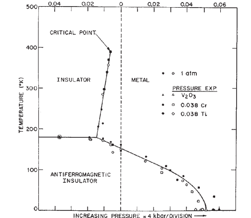
Figure 9: Experimental phase diagram of V₂O₃ doped with Cr and Ti [reproduced from Ref. 68]. Doping V₂O₃ effects the lattice constants in a similar way as applying pressure (generated either by a hydrostatic pressure $P$, or by changing the $V$-concentration from V₂O₃ to V_2-yO₃) and leads to a Mott-Hubbard transition between the paramagnetic insulator (PI) and metal (PM). At lower temperatures, a Mott-Heisenberg transition between the paramagnetic metal (PM) and the antiferromagnetic insulator (AFI) is observed.

Both the paramagnetic metal V₂O₃ and the paramagnetic insulator ${\rm(V_{0.962}Cr_{0.038})_{2}O_{3}}$ have the same corundum crystal structure with only slightly different lattice parameters. [72, 73] Nevertheless, within LDA both phases are found to be metallic (see Fig. 10). The LDA DOS shows a splitting of the five Vanadium d-orbitals into three $t_{2g}$ states near the Fermi energy and two $e_{g}^{\sigma}$ states at higher energies. This reflects the (approximate) octahedral arrangement of oxygen around the vanadium atoms. Due to the trigonal symmetry of the corundum structure the $t_{2g}$ states are further split into one $a_{1g}$ band and two degenerate $e_{g}^{\pi}$ bands, see Fig. 10. The only visible difference between ${\rm(V_{0.962}Cr_{0.038})_{2}O_{3}}$ and ${\rm V_{2}O_{3}}$ is a slight narrowing of the $t_{2g}$ and $e_{g}^{\sigma}$ bands by $\approx 0.2$ and $0.1$ eV, respectively as well as a weak downshift of the centers of gravity of both groups of bands for ${\rm V_{2}O_{3}}$. In particular, the insulating gap of the Cr-doped system is seen to be missing in the LDA DOS. Here we will employ LDA+DMFT(QMC) to show explicitly that the insulating gap is caused by the electronic correlations.

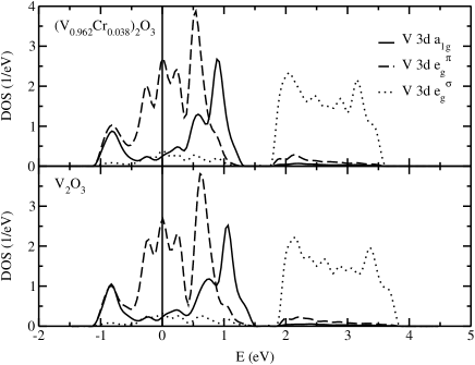
Figure 10: Left: Scheme of the $3d$ levels in the corundum crystal structure. Right: Partial LDA DOS of the 3d bands for paramagnetic metallic ${\rm V_{2}O_{3}}$ and insulating ${\rm(V_{0.962}Cr_{0.038})_{2}O_{3}}$ [reproduced from Ref.44].

In particular, we make use of the simplification for transition metal oxides described in Section 2.7 and restrict the LDA+DMFT(QMC) calculation to the three $t_{2g}$ bands at the Fermi energy, separated from the $e_{g}^{\sigma}$ and oxygen bands.

While the Hund’s rule coupling $J$ is insensitive to screening effects and may, thus, be obtained within LDA to a good accuracy ($J=0.93$ eV [25]), the LDA-calculated value of the Coulomb repulsion $U$ has a typical uncertainty of at least 0.5 eV[24]. To overcome this uncertainty, we study the spectra obtained by LDA+DMFT(QMC) for three different values of the Hubbard interaction ($U=4.5,5.0,5.5$) in Fig. 11. All QMC results presented were obtained for $T\!=\!0.1$ eV. However, simulations for V₂O₃ at $U\!=\!5$ eV, $T\!=\!0.143$ eV, and $T\!=\!0.067$ eV suggest only a minor smoothing of the spectrum with increasing temperature. From the results obtained we conclude that the critical value of $U$ for the MIT is at about $5$ eV: At $U=4.5$ eV one observes pronounced quasiparticle peaks at the Fermi energy, i.e., characteristic metallic behavior, even for the crystal structure of the insulator ${\rm(V_{0.962}Cr_{0.038})_{2}O_{3}}$, while at $U=5.5$ eV the form of the calculated spectral function is typical for an insulator for both sets of crystal structure parameters. At $U=5.0$ eV one is then at, or very close to, the MIT since there is a pronounced dip in the DOS at the Fermi energy for both $a_{1g}$ and $e_{g}^{\pi}$ orbitals for the crystal structure of ${\rm(V_{0.962}Cr_{0.038})_{2}O_{3}}$, while for pure ${\rm V_{2}O_{3}}$ one still finds quasiparticle peaks. (We note that at $T\approx 0.1$ eV one only observes metallic-like and insulator-like behavior, with a rapid but smooth crossover between these two phases, since a sharp MIT occurs only at lower temperatures[39, 71]). The critical value of the Coulomb interaction $U\approx 5$ eV is in reasonable agreement with the values determined spectroscopically by fitting to model calculations, and by constrained LDA, see [44] for details.

Figure 11: LDA+DMFT(QMC) spectra for paramagnetic ${\rm(V_{0.962}Cr_{0.038})_{2}O_{3}}$ (“ins.”) and ${\rm V_{2}O_{3}}$ (“met.”) at $U=4.5$, $5$ and $5.5$ eV, and $T=0.1$ eV $\approx 1000$ K [reproduced from Ref.44].

To compare with the photoemission spectrum of ${\rm V_{2}O_{3}}$ spectrum by Schramme et al.[74] and by Kim et al.[75] as well as with the X-ray absorption data by Müller et al.[76], the LDA+DMFT(QMC) spectrum of Fig. 11 is multiplied with the Fermi function at $T=0.1$ eV and Gauss-broadened by $0.05$ eV to account for the experimental resolution. The theoretical result for $U=5$ eV is seen to be in good agreement with experiment (Fig. 12). In contrast to the LDA results, our results not only describe the different bandwidths above and below the Fermi energy ($\approx 6$ eV and $\approx 2-3$ eV, respectively), but also the position of two (hardly distinguishable) peaks below the Fermi energy (at about -1 eV and -0.3 eV) as well as the pronounced two-peak structure above the Fermi energy (at about 1 eV and 3-4 eV). While LDA also gives two peaks below and above the Fermi energy, their position and physical origin is quite different. Within LDA+DMFT(QMC) the peaks at -1 eV and 3-4 eV are the incoherent Hubbard bands induced by the electronic correlations whereas in the LDA the peak at 2-3 eV is caused by the $e_{g}^{\sigma}$ states and that at -1 eV is the band edge maximum of the $a_{1g}$ and $e_{g}^{\pi}$ states (see Fig. 10). Note that the theoretical and experimental spectrum is highly asymmetric w.r.t the Fermi energy. This high asymmetry which is caused by the orbital degrees of freedom is missing in the one-band Hubbard model which was used by Rozenberg et al.[77] to describe the optical spectrum of ${\rm V_{2}O_{3}}$.

The comparison between theory and experiment for Cr-doped insulating ${\rm V_{2}O_{3}}$ is not as good as for metallic ${\rm V_{2}O_{3}}$, see Ref. 75. This might be, among other reasons, due to the different Cr-doping of experiment and theory, the difference in temperatures (which is important because the insulating gap of a Mott insulator is filled when increasing the temperature [71]), or the fact that every V ion has a unique neighbor in one direction, i.e., the LDA supercell calculation has a pair of V ions per unit cell. The latter aspect has so far not been included but arises naturally when one goes from the simplified calculation scheme described in Section 2.7 (and employed in the present Section with different self-energies for the $a_{1g}$ and $e_{g}^{\pi}$ bands) to a full Hamiltonian calculation.

Figure 12: Comparison of the LDA+DMFT(QMC) spectrum[44] at $U=5\,$eV and $T=0.1$ eV $\approx 1000$ K below (left Figure) and above (right Figure) the Fermi energy (at 0 eV) with the LDA spectrum[44] and the experimental spectrum (left: photoemission spectrum of Schramme et al. [74] and Kim et al. [75]; right: X-ray absorption spectrum of Müller et al. [76]).

Particularly interesting are the spin and the orbital degrees of freedom in ${\rm V_{2}O_{3}}$. From our calculations[44], we conclude that the spin state of ${\rm V_{2}O_{3}}$ is $S=1$ throughout the Mott-Hubbard transition region. This agrees with the measurements of Park et al.[78] and also with the data for the high-temperature susceptibility [79]. But, it is at odds with the $S\!=\!1/2$ model by Castellani et al.[80] and with the results for a one-band Hubbard model which corresponds to $S\!=\!1/2$ in the insulating phase and, contrary to our results, shows a substantial change of the local magnetic moment at the MIT[71]. For the orbital degrees of freedom we find a predominant occupation of the $e_{g}^{\pi}$ orbitals, but with a significant admixture of $a_{1g}$ orbitals. This admixture decreases at the MIT: in the metallic phase we determine the occupation of the ($a_{1g}$, $e_{g1}^{\pi}$, $e_{g2}^{\pi}$) orbitals as (0.37, 0.815, 0.815), and in the insulating phase as (0.28, 0.86, 0.86). This should be compared with the experimental results of Park et al.[78]. From their analysis of the linear dichroism data the authors concluded that the ratio of the configurations $e_{g}^{\pi}e_{g}^{\pi}$:$e_{g}^{\pi}a_{1g}$ is equal to 1:1 for the paramagnetic metallic and 3:2 for the paramagnetic insulating phase, corresponding to a one-electron occupation of (0.5,0.75,0.75) and (0.4,0.8,0.8), respectively. Although our results show a somewhat smaller value for the admixture of $a_{1g}$ orbitals, the overall behavior, including the tendency of a decrease of the $a_{1g}$ admixture across the transition to the insulating state, are well reproduced.

In the study above, the experimental crystal parameters of ${\rm V_{2}O_{3}}$ and ${\rm(V_{0.962}Cr_{0.038})_{2}O_{3}}$ have been taken from the experiment. This leaves the question unanswered whether a change of the lattice is the driving force behind the Mott transition, or whether it is the electronic Mott transition which causes a change of the lattice. For another system, Ce, we will show in Section 5 that the energetic changes near a Mott transition are indeed sufficient to cause a first-order volume change.

5 The Cerium volume collapse: An example for a $4f$-electron system

Cerium exhibits a transition from the $\gamma$- to the $\alpha$-phase with increasing pressure or decreasing temperature. This transition is accompanied by an unusually large volume change of 15% [81], much larger than the 1-2% volume change in ${\rm V_{2}O_{3}}$. The $\gamma$-phase may also be prepared in metastable form at room temperature in which case the reverse $\gamma$-$\alpha$ transition occurs under pressure [82]. Similar volume collapse transitions are observed under pressure in Pr and Gd (for a recent review see Ref. 83). It is widely believed that these transitions arise from changes in the degree of $4f$ electron correlation, as is reflected in both the Mott transition[84] and the Kondo volume collapse (KVC)[85] models.

The Mott transition model envisions a change from itinerant, bonding character of the $4f$-electrons in the $\alpha$-phase to non-bonding, localized character in the $\gamma$-phase, driven by changes in the $4f$-$4f$ inter-site hybridization. Thus, as the ratio of the $4f$ Coulomb interaction to the $4f$-bandwidth increases, a Mott transition occurs to the $\gamma$-phase, similar to the Mott-Hubbard transition of the 3d-electrons in ${\rm V_{2}O_{3}}$ (Section 4).

The Kondo volume collapse[85] scenario ascribes the collapse to a strong change in the energy scale associated with the screening of the local $4f$-moment by conduction electrons (Kondo screening), which is accompanied by the appearance of an Abrikosov-Suhl-like quasiparticle peak at the Fermi level. In this model the $4f$-electron spectrum of Ce would change across the transition in a fashion very similar to the Mott scenario, i.e., a strong reduction of the spectral weight at the Fermi energy should be observed in going from the $\alpha$- to the $\gamma$-phase. The subtle difference comes about by the $\gamma$-phase having metallic $f$-spectra with a strongly enhanced effective mass as in a heavy fermion system, in contrast to the $f$-spectra characteristic of an insulator in the case of the Mott scenario. The $f$-spectra in the Kondo picture also exhibit Hubbard side-bands not only in the $\gamma$-phase, but in the $\alpha$-phase as well, at least close to the transition. While local-density and static mean-field theories correctly yield the Fermi-level peaks in the $f$-spectra for the $\alpha$-phase, they do not exhibit such additional Hubbard side-bands, which is sometimes taken as characteristic of the “$\alpha$-like” phase in the Mott scenario [84]. However, this behavior is more likely a consequence of the static mean-field treatment, as correlated solutions of both Hubbard and periodic Anderson models exhibit such residual Hubbard side-bands in the $\alpha$-like regimes [86].

Typically, the Hubbard model and the periodic Anderson model are considered as paradigms for the Mott and KVC model, respectively. Although both models describe completely different physical situations it was shown recently that one can observe a surprisingly similar behavior at finite temperatures: the evolution of the spectrum and the local magnetic moment with increasing Coulomb interaction show very similar features as well as, in the case of a periodic Anderson model with nearest neighbor hybridization, the phase diagram and the charge compressibility [86, 87]. From this point of view the distinction between the two scenarios appears to be somewhat artificial, at least at temperatures relevant for the description of the $\alpha$-$\gamma$ transition.

For a realistic calculation of the Cerium $\alpha$-$\gamma$ transition, we employ the full Hamiltonian calculation described in Sections 2.2, 2.3, and 2.4 where the one-particle Hamiltonian was calculated by LDA and the $4f$ Coulomb interaction $U$ along with the associated $4f$ site energy shift by a constrained LDA calculation (for details of the the two independent calculations presented in the current Section see Refs. 83, 51 and Ref. 50). We have not included the spin-orbit interaction which has a rather small impact on LDA results for Ce, nor the intra-atomic exchange interaction which is less relevant for Ce as occupations with more than one $4f$-electron on the same site are rare. Furthermore, the $6s$-, $6p$-, and $5d$-orbitals are assumed to be non-interacting in the formalism of Eq. (13), Section 2.3. Note, that the $4f$ orbitals are even better localized than the $3d$ orbitals and, thus, uncertainties in $U$ are relatively small and would only translate into a possible volume shift for the $\alpha$-$\gamma$-transition.

The LDA+DMFT(QMC) spectral evolution of the Ce $4f$-electrons is presented in Fig. 13. It shows similarities to ${\rm V_{2}O_{3}}$ (Fig. 11, Section 4): At a volume per atom $V\!=\!20\,$ų, Fig. 13 shows that almost the entire spectral weight lies in a large quasiparticle peak with a center of gravity slightly above the chemical potential. This is similar to the LDA solution, however, a weak upper Hubbard band is also present even at this small volume. At the volumes $29$ ų and $34$ ų which approximately bracket the $\alpha$-$\gamma$ transition, the spectrum has a three peak structure. Finally, by $V\!=\!46$  ų, the central peak has disappeared leaving only the lower and upper Hubbard bands. However, an important difference to ${\rm V_{2}O_{3}}$ is that the $spd$-spectrum shows metallic behavior and, thus, Cerium remains a metal throughout this transition monitored by a vanishing $4f$ quasiparticle resonance.

Figure 13: Evolution of the $4f$ spectral function $A(\omega)$ with volume at $T\!=\!0.136\>$eV ($\omega\!=\!0$ corresponds to the chemical potential; curves are offset as indicated; $\Delta\tau\!=\!0.11\!$ eV^-1). Coinciding with the sharp anomaly in the correlation energy (Fig. 14), the central quasiparticle resonance disappears, at least at finite temperatures [reproduced from Ref. 51].

To study the energetic changes associated with the rapid change of the quasiparticle weight at the Fermi energy, we calculate the DMFT energy per site for the model Hamiltonian (13)

$$E_{\rm DMFT} \!=\! \frac{T}{N_{k}}\sum_{n{\bf k}\sigma}{\rm Tr}({H}^{0}_{\rm LDA}({\bf k}){G}_{\bf k}(i\omega_{n}))e^{i\omega_{n}0^{+}}+U_{f}\,d.$$ (47)

Here, Tr denotes the trace over the $16\times 16$ matrices, $T$ the temperature, $N_{k}$ the number of ${\bf k}$ points, $G_{\bf k}$ the Green function matrix w.r.t. the orbital indices, ${H}^{0}_{\rm LDA}({\bf k})$ the LDA one-particle matrix Eq. (17), and

$$d=\frac{1}{2}{\sum}_{m\sigma,m^{\prime}\sigma^{\prime}}^{\prime}\langle\hat{n}_{ifm\sigma}\,\hat{n}_{ifm^{\prime}\sigma^{\prime}}\rangle$$ (48)

is a generalization of the one-band double occupation for multi-band models.

Fig. 14a shows our calculated DMFT(QMC) energies $E_{\rm DMFT}$ as a function of atomic volume at three temperatures relative to the paramagnetic Hartree Fock (HF) energies $E_{\rm PMHF}$ [of the Hamiltonian (13)], i.e., the energy contribution due to electronic correlations. Similarly given are the polarized HF energies which reproduce $E_{\rm DMFT}$ at large volumes and low temperatures. With decreasing volume, however, the DMFT energies bend away from the polarized HF solutions. Thus, at $T\!=\!0.054\,$eV$\,\approx 600\,$K, a region of negative curvature in $E_{\rm DMFT}\!-\!E_{\rm PMHF}$ is evident within the observed two phase region (arrows).

Figure 14: (a) Correlation energy $E_{\rm DMFT}\!-\!E_{\rm PMHF}$ as a function of atomic volume (symbols) and polarized HF energy $E_{\rm AFHF}\!-\!E_{\rm PMHF}$ (dotted lines which, at large V, approach the DMFT curves for the respective temperatures); arrows: observed volume collapse from the $\alpha$- to the $\gamma$-phase. The correlation energy sharply bends away from the polarized HF energy in the region of the transition. (b) The resultant negative curvature leads to a growing depression of the total energy near $V\!=\!26$–$28$ ų as temperature is decreased, consistent with an emerging double well at still lower temperatures and thus the $\alpha$-$\gamma$ transition. The curves at $T=0.544\,$eV were shifted downwards in (b) by $-0.5\,$eV to match the energy range [reproduced from Ref. 51].

Fig. 14b presents the calculated LDA+DMFT total energy $E_{\rm tot}(T)\!=\!E_{\rm LDA}(T)\!+\!E_{\rm DMFT}(T)\!-\!E_{\rm mLDA}(T)$ where $E_{\rm mLDA}$ is the energy of an LDA-like solution of the Hamiltonian (13) [88]. Since both $E_{\rm LDA}$ and $E_{\rm PMHF}\!-\!E_{\rm mLDA}$ have positive curvature throughout the volume range considered, it is the negative curvature of the correlation energy in Fig. 14a which leads to the dramatic depression of the LDA+DMFT total energies in the range $V\!=\,$26-28 ų for decreasing temperature, which contrasts to the smaller changes near $V\!\!=\!34\,$ų in Fig. 14b. This trend is consistent with a double well structure emerging at still lower temperatures (prohibitively expensive for QMC simulations), and with it a first-order volume collapse. This is in reasonable agreement with the experimental volume collapse given our use of energies rather than free energies, the different temperatures, and the LDA and DMFT approximations. A similar scenario has been proposed recently for the $\delta$-$\alpha$ transition in Pu on the basis of LDA+DMFT calculations [48], which solves DMFT by an ansatz inspired by IPT and includes a modification of the DFT/LDA step to account for the density changes introduced by the DMFT[49].

In a separate LDA+DMFT(NCA) calculation for Ce, we have obtained a number of physical quantities for both phases which may be compared to experimental values [50]. Various static properties extracted

	$\alpha$-CeTheo	$\alpha$-Ce[89, 90]	$\gamma$-CeTheo	$\gamma$-Ce [89, 90]
$P_{0}$	0.126	0.1558	0.0150	0.0426
$P_{1}$	0.829	0.8079	0.9426	0.9444
$P_{2}$	0.044	0.0264	0.0423	0.0131
$n_{f}$	0.908	$0.8\ldots 0.861$	1.014	$0.971\ldots 1$
$T_{K}$, [K]	1000	$945\ldots 2000$	30	$60\ldots 95$
$\chi$, [$10^{-3}emu/mol$]	1.08	$0.53\ldots 0.70$	24	$8.0\ldots 12$

Table 1: Comparison between LDA+DMFT(NCA) calculated parameters for both $\alpha$- and $\gamma$-phase at $T=580~{}K$ and experimental values[89, 90] [reproduced from Ref. 50]. $P_{0}$, $P_{1}$ and $P_{2}$ are partial probabilities for an empty, singly and doubly occupied $4f$-state, $n_{f}$ is the $f$-electron occupancy, $T_{\rm K}$ the estimated Kondo temperature, and $\chi$ the magnetic susceptibility.

from the calculations[50] and their counterparts from experiments are collected in Table 1 and show an overall fair to good agreement in the tendencies and, except for the susceptibility, the absolute values. Since the calculation of the magnetic susceptibility $\chi$ in Ref. 50 was based on simplifying assumptions, the absolute numbers cannot be expected to match experiment. However, the general tendency and especially the ratio between $\alpha$- and $\gamma$-Ce is in good agreement with experiment. It is interesting to note that the experiments predict a

Figure 15: Comparison between combined photoemission [91] and BIS [92] experimental (circles) and theoretical (solid line) $f$-spectra for $\alpha$- (upper part) and $\gamma$-Ce (lower part) at $T=580\,$K. The relative intensities of the BIS and photoemission portions are roughly for one 4$f$ electron. The experimental and theoretical spectra were normalized and the theoretical curve was broadened with resolution width of $0.4\,$eV. In the insets a comparison between RIPES [93] experimental (circles) and theoretical (solid line) $f$-spectra is given. The experimental and theoretical data were normalized and the theoretical curve was broadened with broadening coefficient of $0.1\,$eV [reproduced from Ref. 50].

finite Kondo screening-scale for both phases, which actually would point toward the KVC scenario. Finally, let us compare spectral functions for the $4f$-states calculated with the LDA+DMFT(NCA) approach to experimental data[91]. The photoemission spectrum for $\alpha$-Ce (upper part of Fig. 15) shows a main structure between $3\>$eV and $7\>$eV, which is attributed to $4f^{2}$ final state multiplets. In the calculated spectrum all excitations to $4f^{2}$ states are described by the featureless upper Hubbard band. As a consequence of the simplified interaction model all doubly occupied states are degenerate. This shortcoming in our calculation is responsible for the sharply peaked main structure. The neglected exchange interaction would produce a multiplet structure, which would be closer to the experiment. The experimental peak at about $0.5\>$eV is attributed to two $4f^{1}$ final states, which are split by spin-orbit coupling. The calculated $f$-spectrum shows a sharp quasiparticle or Kondo resonance slightly above the Fermi energy, which is the result of the formation of a singlet state between $f$- and conduction states. We thus suggest that the spectral weight seen in the experiment is a result of this quasiparticle resonance. Since we did not yet include spin-orbit coupling in our model, we cannot observe the mentioned splitting of the resonance. However, as it is well known [94], the introduction of such a splitting would eventually split the Kondo resonance. If we used the experimentally determined value of about $0.3\>$eV for the spin-orbit splitting [92], the observed resonance of width $0.5\>$eV would indeed occur in the calculations. In the lower part of Fig. 15, a comparison between experiment and our calculation for $\gamma$-Ce is shown. The most striking difference between lower and upper part of Fig. 15 is the absence of the Kondo resonance in the high temperature phase ($\gamma$-Ce; transition temperature $141~{}K$ [81]) which is in agreement with our calculations.

In the insets of Fig. 15, our results for the non-occupied states in the $f$-density are compared with RIPES data [93]. The calculated $f$-spectra were multiplied by the Fermi-step function and broadened with an Lorentzian of the width $0.1\,$eV in order to mimic the experimental resolution in the theoretical curves. Here, as above the theoretical overestimation of the sharpness of the upper Hubbard band is a consequence of the simplified local interaction and thus of the missing multiplet structure of the $4f^{2}$-final states. The main feature of the experimental spectra, i.e., a strong decrease of the intensity ratio for Kondo resonance and upper Hubbard band peaks from $\alpha$- to $\gamma$-Ce, can also be seen in the theoretical curves of Fig. 15 as well as in the study presented in Fig. 13. A more thorough comparison of these two independent LDA+DMFT(NCA) and LDA+DMFT(QMC) studies remains to be done.

6 Conclusion and Outlook

In this paper we discussed the set-up of the computational scheme LDA+DMFT which merges two non-perturbative, complementary investigation techniques for many-particle systems in solid state physics. LDA+DMFT allows one to perform ab initio calculations of real materials with strongly correlated electrons. Using the band structure results calculated within local density approximation (LDA) as input, the missing electronic correlations are introduced by dynamical mean-field theory (DMFT). On a technical level this requires the solution of an effective self-consistent, multi-band Anderson impurity problem by some numerical method (e.g. IPT, NCA, QMC). Comparison of the photoemission spectrum of La_1-xSr_xTiO₃ calculated by LDA+DMFT using IPT, NCA, and QMC reveal that the choice of the evaluation method is of considerable importance. Indeed, only with the numerically exact QMC quantitatively reliable results are obtained. The results of the LDA+DMFT(QMC) approach were found to be in very good agreement with the experimental photoemission spectrum of La_0.94Sr_0.06TiO₃.

We also presented results of a LDA+DMFT(QMC) study[44] of the Mott-Hubbard metal-insulator transition (MIT) in the paramagnetic phase of (doped) $\mathrm{V_{2}O_{3}}$. These results showed a Mott-Hubbard MIT at a reasonable value of the Coulomb interaction $U\approx 5$eV and are in very good agreement with the experimentally determined photoemission and X-ray absorption spectra for this system, i.e., above and below the Fermi energy. In particular, we find a spin state $S=1$ in the paramagnetic phase, and an orbital admixture of $e_{g}^{\pi}e_{g}^{\pi}$ and $e_{g}^{\pi}a_{1g}$ configurations, which both agree with recent experiments. Thus, LDA+DMFT(QMC) provides a remarkably accurate microscopic theory of the strongly correlated electrons in the paramagnetic metallic phase of $\mathrm{V_{2}O_{3}}$.

Another material where electronic correlations are considered to be important is Cerium. We reviewed our recent investigations of the Ce $\alpha$-$\gamma$ transition, based on LDA+DMFT(QMC)[51] and LDA+DMFT(NCA)[50] calculations. The spectral results and susceptibilities show the same tendency as seen in the experiment, namely a dramatic reduction in the size of the quasiparticle peak at the Fermi level when passing from the $\alpha$- to the $\gamma$-phase. While we do not know at the moment whether the zero-temperature quasiparticle peak will completely disappear at an even larger volume (i.e., in a rather Mott-like fashion) or simply fade away continuously with increasing volume (i.e., in a more Kondo-like fashion), an important aspect of our results is that the rapid reduction in the size of the peak seems to coincide with the appearance of a negative curvature in the correlation energy and a shallow minimum in the total energy. This suggest that the electronic correlations responsible for the reduction of the quasiparticle peak are associated with energetic changes that are strong enough to cause a volume collapse in the sense of the Kondo volume collapse model[85], or a Mott transition model[84] including electronic correlations.

At present LDA+DMFT is the only available ab initio computational technique which is able to treat correlated electronic systems close to a Mott-Hubbard MIT, heavy fermions, and $f$-electron materials. The physical properties of such systems are characterized by the correlation-induced generation of small, Kondo-like energy scales which require the application of genuine many-body techniques. The appearance of Kondo-like energy scales in strongly correlated systems leads to several experimentally relevant consequences. One of the most important features is the enhancement of the quasiparticle mass m^∗ (i.e., the decrease of the quasiparticle residue Z). This phenomenon can be observed as an enhancement of the coefficient $\gamma$ in the specific heat. Another important characteristic is the Wilson ratio between $\gamma$ and the Pauli spin susceptibility $\chi$. Future LDA+DMFT investigations will determine these quantities for real systems, as well as the optical conductivity, phase-diagrams, the local vertex function, and various susceptibilities.

LDA+DMFT provides, at last, a powerful tool for ab initio investigations of real materials with strong electronic correlations. Indeed, LDA+DMFT depends on the input from both band structure theory and many-body approaches. Hence, for this computational scheme to be entirely successful in the future two strong and vital communities will finally have to join forces.

References

- [1] M. Born und R. Oppenheimer, Ann. Phys. (Leipzig) 84, 457 (1927).
- [2] R. O. Jones and O. Gunnarsson, Rev. Mod. Phys. 61, 689 (1989).
- [3] W. Metzner and D. Vollhardt, Phys. Rev. Lett. 62, 324 (1989).
- [4] E. Müller-Hartmann, Z. Phys. B 74, 507 (1989); ibid. B 76, 211 (1989).
- [5] U. Brandt und C. Mielsch, Z. Phys. B 75, 365 (1989); ibid. B 79, 295 (1989); ibid. B 82, 37 (1991).
- [6] V. Janiš, Z. Phys. B 83, 227 (1991); V. Janiš and D. Vollhardt, Int. J. Mod. Phys. 6, 731 (1992).
- [7] A. Georges and G. Kotliar, Phys. Rev. B 45, 6479 (1992).
- [8] M. Jarrell, Phys. Rev. Lett. 69, 168 (1992).
- [9] D. Vollhardt, in Correlated Electron Systems, edited by V. J. Emery, World Scientific, Singapore, 1993, p. 57.
- [10] Th. Pruschke, M. Jarrell, and J. K. Freericks, Adv. in Phys. 44, 187 (1995).
- [11] A. Georges, G. Kotliar, W. Krauth, and M. J. Rozenberg, Rev. Mod. Phys. 68, 13 (1996).
- [12] V. I. Anisimov, A. I. Poteryaev, M. A. Korotin, A. O. Anokhin, and G. Kotliar, J. Phys. Cond. Matter 9, 7359 (1997).
- [13] An introduction to LDA+DMFT less complete than the present Proceedings has been given in K. Held, I. A. Nekrasov, N. Blümer, V. I. Anisimov, and D. Vollhardt, Int. J. Mod. Phys. B 15, 2611 (2001).
- [14] P. Hohenberg and W. Kohn, Phys. Rev. B 136, 864 (1964).
- [15] M. Levy, Proc. Natl. Acad. Sci. (USA), 76, 6062 (1979).
- [16] W. Kohn and L. J. Sham, Phys. Rev. 140, 4A, A1133 (1965); W. Kohn and L. J. Sham, Phys. Rev. A - Gen.Phys. 140, 1133 (1965); L. J. Sham and W. Kohn, Phys. Rev. 145 N 2, 561 (1966).
- [17] L. Hedin and B. Lundqvist, J. Phys. C: Solid State Phys. 4, 2064 (1971); U. von Barth and L. Hedin, J. Phys. C: Solid State Phys. 5, 1629 (1972).
- [18] D. M. Ceperley and B. J. Alder, Phys. Rev. Lett. 45, 566 (1980).
- [19] O. K. Andersen, Phys. Rev. B 12, 3060 (1975); O. Gunnarsson, O. Jepsen, and O. K. Andersen, Phys. Rev. B 27, 7144 (1983); O. K. Andersen and O. Jepsen, Phys. Rev. Lett. 53, 2571 (1984).
- [20] T. C. Leung, X. W. Wang, and B. N. Harmon, Phys. Rev. B 37, 384 (1988); W. E. Pickett, Rev. Mod. Phys. 61, 433 (1989).
- [21] J. Wahle, N. Blümer, J. Schlipf, K. Held, and D. Vollhardt, Phys. Rev. B 58, 12749 (1998).
- [22] V. I. Anisimov, J. Zaanen, and O. K. Andersen, Phys. Rev. B 44, 943 (1991); V. I. Anisimov, F. Aryasetiawan, and A. I. Lichtenstein, J. Phys. Cond. Matter 9, 767 (1997).
- [23] O. Gunnarson, O. K. Andersen, O. Jepsen, and J. Zaanen, Phys. Rev. B 39, 1708 (1989).
- [24] I. A. Nekrasov, K. Held, N. Blümer, A. I. Poteryaev, V. I. Anisimov, and D. Vollhardt, Euro. Phys. J. B 18, 55 (2000).
- [25] I. Solovyev, N. Hamada, and K. Terakura, Phys. Rev. B 53, 7158 (1996).
- [26] A. I. Lichtenstein and M. I. Katsnelson, Phys. Rev. B 57, 6884 (1998).
- [27] V. Drchal, V. Janiš, and J. Kudrnovský, in Electron Correlations and Material Properties, edited by A. Gonis, N. Kioussis, and M. Ciftan, Kluwer/Plenum, New York, 1999, p. 273.
- [28] J. Lægsgaard and A. Svane, Phys. Rev. B 58, 12817 (1998).
- [29] Th. Wolenski, Combining bandstructure and dynamical mean-field theory: A new perspective on V2O3, Ph.D. Thesis, Universität Hamburg 1998 (Shaker Verlag, Aachen, 1999).
- [30] M. B. Zölfl, Th. Pruschke, J. Keller, A. I. Poteryaev, I. A. Nekrasov, and V. I. Anisimov, Phys. Rev. B 61, 12810 (2000).
- [31] P. W. Anderson, in Moment formation in solids, edited by W. J. L. Buyers, Plenum Press, New York and London, 1984, p. 313.
- [32] H. Keiter and J. C. Kimball, Phys. Rev. Lett. 25, 672 (1970); N. E. Bickers, D. L. Cox, and J. W. Wilkins, Phys. Rev. B 36, 2036 (1987).
- [33] Th. Pruschke and N. Grewe, Z. Phys. B 74, 439 (1989).
- [34] Th. Pruschke, D. L. Cox, and M. Jarrell, Phys. Rev. B 47, 3553 (1993).
- [35] J. E. Hirsch and R. M. Fye, Phys. Rev. Lett. 56, 2521 (1986); M. Jarrell, Phys. Rev. Lett. 69, 168 (1992); M. Rozenberg, X. Y. Zhang, and G. Kotliar, Phys. Rev. Lett. 69, 1236 (1992); A. Georges and W. Krauth, Phys. Rev. Lett. 69, 1240 (1992); M. Jarrell, in Numerical Methods for Lattice Quantum Many-Body Problems, edited by D. Scalapino, Addison Wesley, 1997.
- [36] M. Caffarel and W. Krauth, Phys. Rev. Lett. 72, 1545 (1994).
- [37] R. Bulla, Adv. Sol. State Phys. 46, 169 (2000).
- [38] H. Kajueter and G. Kotliar, Int. J. Mod. Phys. 11, 729 (1997).
- [39] M. J. Rozenberg, Phys. Rev. B 55, R4855 (1997).
- [40] J. E. Han, M. Jarrell, and D. L. Cox, Phys. Rev. B 58, R4199 (1998).
- [41] K. Held and D. Vollhardt, Euro. Phys. J. B 5, 473 (1998).
- [42] M. I. Katsnelson and A. I. Lichtenstein, J. Phys. Cond. Matter 11, 1037 (1999).
- [43] M. I. Katsnelson and A. I. Lichtenstein, Phys. Rev. B 61, 8906 (2000).
- [44] K. Held, G. Keller, V. Eyert, V. I. Anisimov, and D. Vollhardt, Phys. Rev. Lett. 86, 5345 (2001).
- [45] A. Liebsch and A. I. Lichtenstein, Phys. Rev. Lett. 84, 1591 (2000).
- [46] V. I. Anisimov, I. A. Nekrasov, D. E. Kondakov, T. M. Rice, and M. Sigrist, cond-mat/0011460, ibid. cond-mat/0107095 (2001).
- [47] A. I. Lichtenstein, M. I. Katsnelson, and G. Kotliar 87, 67205 (2001).
- [48] S. Y. Savrasov, G. Kotliar, and E. Abrahams, Nature 410, 793 (2001).
- [49] S. Y. Savrasov and G. Kotliar, cond-mat/0106308.
- [50] M. B. Zölfl, I. A. Nekrasov, Th. Pruschke, V. I. Anisimov, and J. Keller, Phys. Rev. Lett. (in press), cond-mat/0101280.
- [51] K. Held, A. K. McMahan, and R. T. Scalettar, Phys. Rev. Lett. (in press), cond-mat/0106599; A. K. McMahan, K. Held, and R. T. Scalettar, in preparation.
- [52] W. Weber, J. Bünemann, and F. Gebhard, in Band-Ferromagnetism, edited by K. Baberschke, M. Donath, and W. Nolting, Lecture Notes in Physics, Vol. 580 (Springer, Berlin, 2001), p. 9; J. Bünemann, F. Gebhard, W. Weber, Phys. Rev. B 57, 6896 (1998).
- [53] M. Suzuki, Prog. Theor. Phys. 56, 1454 (1976)
- [54] One limitation of QMC is that it is very difficult to deal with the spin-flip term of the Hund’s rule coupling because of a “minus-sign problem” which arises in a Hubbard-Stratonovich decoupling of this spin-flip term, see K. Held, Ph.D. thesis Universität Augsburg 1999 (Shaker Verlag, Aachen, 1999). In the particle-hole symmetric case another decoupling scheme which includes the spin-flip term is possible without “minus-sign problem”, see Y. Motome and M. Imada, J. Phys. Soc. Jap. 66, 1872 (1997).
- [55] N. Metropolis, A. W. Rosenbluth, M. N. Rosenbluth, A. H. Teller, and E. Teller, J. Chem. Phys. 21, 1087 (1953).
- [56] M. Jarrell and J. E. Gubernatis, Physics Reports 269, 133 (1996).
- [57] E. Müller-Hartmann, Z. Phys. B 57, 281 (1984).
- [58] G. Kotliar, Physica B 259-261, 711 (1999). R. Chitra and G. Kotliar, Phys. Rev. B 62, 12715 (2000).
- [59] D. A. MacLean, H.-N. Ng, and J. E. Greedan, J. Solid State Chem. 30, 35 (1979).
- [60] M. Eitel and J. E. Greedan, Journal of the Less-Common Metals 116, 95 (1986).
- [61] J. P. Gopel, J. E. Greedan, and D. A. MacLean, J. Solid State Chem. 43, 244 (1981).
- [62] Y. Okimoto, T. Katsufuji, Y. Okada, T. Arima, and Y. Tokura, Phys. Rev. B 51, 9581 (1995).
- [63] W. Heindl, Th. Pruschke, and J. Keller, J. Phys. – Condens. Matter 12, 2245 (2000).
- [64] A. Fujimori et al, Phys. Rev. Lett. 69, 1796 (1992). A. Fujimori et al, Phys. Rev. B 46, 9841 (1992). A qualitatively and quantitatively similar spectrum was obtained recently by Yoshida et al., cond-mat/9911446, with an experimental energy resolution of only 30 meV. One may suppose, however, that broadening effects due to the polycrystalline nature of the sample and surface effects are, then, larger than the instrumental resolution.
- [65] At present, QMC simulations of the DMFT equations are not feasible at the experimental temperature (80K). We note, however, that no intrinsic temperature dependence was observed in the experiment[64], at least up to room temperature.
- [66] B. Keimer, D. Casa, A. Ivanov, J.W. Lynn, M. v. Zimmermann, J.P. Hill, D. Gibbs, Y. Taguchi, and Y. Tokura, Phys. Rev. Lett. 85, 3946 (2000).
- [67] N. F. Mott, Rev. Mod. Phys. 40, 677 (1968); Metal-Insulator Transitions (Taylor & Francis, London, 1990); F. Gebhard, The Mott Metal-Insulator Transition (Springer, Berlin, 1997).
- [68] D. B. McWahn et al., Phys. Rev. B 7, 1920 (1973).
- [69] J. Hubbard, Proc. Roy. Soc. London Ser. A 276, 238 (1963); 277, 237 (1963); 281, 401 (1964).
- [70] W. F. Brinkman and T. M. Rice, Phys. Rev. B 2, 4302 (1970).
- [71] G. Moeller, Q. Si, G. Kotliar, and M. Rozenberg, Phys. Rev. Lett. 74, 2082 (1995); J. Schlipf, M. Jarrell, P. G. J. van Dongen, N. Blümer, S. Kehrein, Th. Pruschke, and D. Vollhardt, Phys. Rev. Lett. 82, 4890 (1999); M. J. Rozenberg, R. Chitra, and G. Kotliar, Phys. Rev. Lett. 83, 3498 (1999); R. Bulla, Phys. Rev. Lett. 83, 136 (1999); R. Bulla, T. A. Costi, and D. Vollhardt, Phys. Rev. B 64, 45103 (2001).
- [72] P. D. Dernier, J. Phys. Chem. Solids 31, 2569 (1970).
- [73] Use of the crystal structure of Cr-doped for the insulating phase of pure is justified by the observation that Cr-doping is equivalent to the application of (negative) pressure.
- [74] M. Schramme, Ph.D. thesis, Universität Augsburg 2000 (Shaker Verlag, Aachen, 2000); M. Schramme et al. (unpublished).
- [75] H.-D. Kim, J.-H. Park, J. W. Allen, A. Sekiyama, A. Yamasaki, K. Kadono, S. Suga, Y. Saitoh, T. Muro, and P. Metcalf, cond-mat/0108044.
- [76] O. Müller, J. P. Urbach, E. Goering, T. Weber, R. Barth, H. Schuler, M. Klemm, S. Horn, and M. L. denBoer, Phys. Rev. B 56, 15056 (1997).
- [77] M. J. Rozenberg, G. Kotliar, H. Kajueter, G. A. Thomas, D. H. Rapkine, J. M. Honig, and P. Metcalf, Phys. Rev. Lett. 75, 105 (1995).
- [78] J.-H. Park, L. H. Tjeng, A. Tanaka, J. W. Allen, C. T. Chen, P. Metcalf, J. M. Honig, F. M. F. de Groot, and G. A. Sawatzky, Phys. Rev. B 61, 11 506 (2000).
- [79] D. J. Arnold and R. W. Mires, J. Chem. Phys. 48, 2231 (1968).
- [80] C. Castellani, C. R. Natoli, and J. Ranninger, Phys. Rev. B 18, 4945 (1978); 18, 4967 (1978); 18, 5001 (1978).
- [81] Handbook on the Physics and Chemistry of Rare Earths, edited by K. A. Gschneider Jr. and L. R. Eyring (North-Holland, Amsterdam, 1978); in particular, D. G. Koskenmaki and K. A. Gschneider Jr., ibid, p.337.
- [82] J. S. Olsen, L. Gerward, U. Benedict, and J.-P. Itié, Physica 133B, 129 (1985).
- [83] A. K. McMahan, C. Huscroft, R. T. Scalettar, and E. L. Pollock, J. Comput.-Aided Mater. Design 5, 131 (1998).
- [84] B. Johansson, Philos. Mag. 30, 469 (1974); B. Johansson, I.A. Abrikosov, M. Aldén, A. V. Ruban, and H.L. Skriver Phys. Rev. Lett. 74, 2335 (1995).
- [85] J. W. Allen and R. M. Martin, Phys. Rev. Lett. 49, 1106, (1982); J. W. Allen and L. Z. Liu, Phys. Rev. B 46, 5047, (1992); M. Lavagna, C. Lacroix, and M. Cyrot, Phys. Lett. 90A, 210 (1982).
- [86] K. Held, C. Huscroft, R.T. Scalettar, and A.K. McMahan, Phys. Rev. Lett. 85, 373 (2000); see also C. Huscroft, A. K. McMahan, and R. T. Scalettar, Phys. Rev. Lett. 82, 2342 (1999).
- [87] K. Held and R. Bulla, Eur. Phys. J. B 17, 7 (2000).
- [88] We solve self-consistently for using a self energy , and then remove this contribution from the eigenvalue sum to get the kinetic energy. The potential energy is taken to be .
- [89] L. Z. Liu, J. W. Allen, O. Gunnarsson, N. E. Christensen, and O. K. Andersen, Phys. Rev. B 45, 8934 (1992).
- [90] A. P. Murani, Z. A. Bowden, A. D. Taylor, R. Osborn, and W. G. Marshall, Phys. Rev B 48, 13981 (1993).
- [91] D. M. Wieliczka, C. G. Olson, and D. W. Lynch, Phys. Rev. B 29, 3028 (1984).
- [92] E. Wuilloud, H. R. Moser, W. D. Schneider, and Y. Baer, Phys. Rev. B 28, 7354 (1983).
- [93] M. Grioni, P. Weibel, D. Malterre, Y. Baer, and L. Duo, Phys. Rev. B 55, 2056 (1997).
- [94] T. A. Costi, Phys. Rev. Lett. 85, 1504 (2000).