Conditions for the importance of inelastic losses in photoemission

Abstract

It is shown that for materials near the metal insulator transition, inelastic losses can give rise to substantial changes on a scale of 10-100 meV in the observed lineshape compared to the intrinsic spectral function of an electron photoemitted from a solid. These changes arise from the frequency dependence of the loss function, similar to those directly observed in electron energy loss experiments. For good metals and insulators, on the other hand, the inelastic losses not important. We derive quantitative conditions to delineate the various cases. We find in particular that La_1.2Sr_1.8Mn₂O₇ does not satisfy these conditions, so that no significant losses are to be expected in this material. This contradicts the reasoning of Schulte et.al [Phys. Rev. B 63, 165429 (2001)], who, on finding no significant lineshape effects in this material, concluded that inelastic losses are always unimportant.

I Introduction

A recent paper by Schulte et al. [1] treats the subject of energy loss by an electron photoemitted from a solid.  Their contention is ”that energy loss processes occurring once the electron is outside the solid contribute only weakly to the spectrum and can in most cases be either neglected or treated as a weak structureless background”.  In particular, they consider the ohmic loss processes suggested by one of us [2] and find that these ”are only a small contribution to the total spectrum”.  They give several arguments to support these statements.  In this communication, we consider these arguments.  We show that, for the systems of interest in this connection, namely those near the metal-insulator transition, the ohmic loss processes can, on the contrary, give a substantial contribution to the spectrum.  This contribution can change the interpretation of experimental data.  This is contrary to the conclusions of Ref. [1]

The conceptual background of the problem is in some ways similar to an ordinary scattering problem. The photoelectron, after absorbing a photon of fixed energy, becomes a part of the ”incident beam” which then scatters from the system on its way to the detector.  Unlike the incident beam in an ordinary well-designed scattering experiment, this beam is not monochromatic.  Indeed, it is the energy distribution of this beam that is of the most experimental interest since it gives the spectrum of the solid. Any part of the beam which undergoes scattering reflects the properties of the system only indirectly and we therefore wish to minimize the effects of this scattering as much as possible.  Unfortunately, one has little control over this scattering, and it is poorly understood in most cases [3].  Furthermore, the inelastic mean free path of electrons at 20 eV, a typical energy for valence-band photoemission (PE), is very short when the electron is in the metal - on the order of a few nm.  That the inelastic scattering is very strong is not surprising since the particle is charged.

It is nevertheless indubitably true that the observed spectrum often faithfully reflects the underlying electronic spectrum of the solid.  For example, in the case of pure elemental metals such as Na, agreement between dispersion relations from band structure calculations and the movement of peaks in angle-resolved photoemission intensities is good.  This is due to a combination of factors.  The relevant energy scales are in electron volts.  The electrons that reach the surface of the solid have either undergone such substantial inelastic scattering that their energies are well below the chemical potential or they have not suffered any inelastic scattering.  In the former case, the electrons may be detected, but because of their very low energies ($\sim eV$ below the chemical potential ) they can easily be separated from the signal.  (Typically, these ”secondaries” are very numerous).  In the latter case, the electrons are candidates for the desired signal, but they must still get to the detector without further scattering.  As long as these additional inelastic losses do not depend strongly on angle or if the losses involve energies that are small compared with the energy scales of interest in the experiment, then they will not distort the observed spectra in an important way.

Ref [2] is an attempt to show how one may correct for the additional inelastic scattering after the electron leaves the surface in valence-band photoemission in cases when such corrections are important.  These questions were further developed in Ref. [5]. In this paper we develop quantitaive criteria to decide when such corrections are important, at least in the special case that a Drude model describes the conductivity.

It is crucial to be aware that whether the corrections are important depends on the resolution of the experiment.  If resolution is 100 meV or greater, as in classic band-mapping experiments, then losses on the order of 10 meV (a more typical scale for ohmic dissipation) are not important.  If one is looking for a gap or pseudogap on the order of 20 meV, then relatively small energy losses (that could be ignored in the 1970’s) become of paramount importance.  The point is that these smaller energy scales can match up with the energy scales associated with the ohmic losses in metals.  It is therefore necessary to investigate losses due to ordinary ohmic dissipation.  Any theory of this phenomenon must be consistent with the many historical successes of PE in measuring dispersion relations and densities of states.  Hopefully a detailed treatment of the inelastic scattering will also throw light on situations where theory and experiment appear currently to be in disagreement.

II General Considerations

In the Born approximation, the probability for electrons to undergo a single inelastic scattering event losing an energy $\hbar\omega$ after it has left the system is

$$P(\omega)=\frac{e^{2}}{\hbar\omega v}\mathop{\rm Im}\left(\frac{-1}{1+\varepsilon(\omega)}\right)=\frac{4\pi e^{2}}{\hbar\omega^{2}v}\,\frac{\mathop{\rm Re}\sigma(\omega)}{|1+\varepsilon(\omega)|^{2}}$$ (1)

This refers to electrons that are emitted normally at a speed $v$ from an isotropic material with dielectric function $\varepsilon(\omega)$ and conductivity $\sigma(\omega).$  In Ref. [2] the prefactor was incorrect.  The correct prefactor was derived by Mills [4].  As pointed out in Ref.[1], there is a sum rule for this function:

$$\int_{0}^{\infty}P(\omega)\,\,d\omega=\frac{\pi}{2}\frac{e^{2}}{\hbar v}.$$ (2)

For a speed $v$ corresponding to 20 eV, we find $\int_{0}^{\infty}P(\omega)\,\,d\omega=0.65.$  The Born approximation is valid only when the total scattering probability is small, indicating that we may be near or beyond the validity of the approximation here. Multiple scattering is possible or indeed probable. In view of the complications introduced by the possibility of multiple scattering, it is important to examine the assumptions made about it.  We look carefully at the consequences of various assumptions.

Assumption (1). Multiple scattering is negligible.  Unitarity then implies that the forward scattering probability is 0.35.  The observed angle-integrated PE intensity is then

$$I(\omega)=0.35\,N(\omega)f(\omega)+\int_{\omega}^{\infty}N(\omega^{\prime})\,f(\omega^{\prime})\,P(\omega^{\prime}-\omega)\,d\omega^{\prime}$$ (3)

Here $N(\omega)$ is the density of states that the experiment sets out to measure. $f(\omega)$ is the Fermi function.  Evidently, the second term is comparable in magnitude to the first.  Let us examine the conditions under which it can be ignored in experiments, (proceeding to subcases of assumption (1)). (a) $P(\omega)$ is a very sharply peaked function about $\omega=0$.  Then the two terms are the same and $N(\omega)$ can be extracted from the data without further ado.  Obviously, this will only work if the width $\Delta(\omega)$ of $P(\omega)$ is much less than the features of the data to be resolved.  If we call the energy width of the narrowest feature in the density of states $R$ , then we need $\Delta(\omega)<<R$.  (b) Most of the weight in $P(\omega)$ is at very high $\omega,$ say at $\omega>\omega_{\max}.$  Let the valence band, or the part of it of experimental interest, be of energy width $B$.  In this case, there will be little overlap in the two terms of Eq. 3 as long as $\omega_{\max}>B$.  By focusing on the appropriate frequency range, we can still extract $N(\omega).$  (c)  $P(\omega)$ is a linear combination of functions satisfying (a) and (b).

If $P(\omega)$ does not satisfy conditions (a), (b), or (c), then certainly it cannot be ignored.  This does not mean that it is impossible to extract $N(\omega),$ merely that substantial deconvolution of the observed intensity will be required.

Assumption (2).  The probability of multiple scattering is of order 1.  Then the observed intensity is

$$I(\omega)=P_{0}\,N(\omega)f(\omega)+\int_{\omega}^{\infty}N(\omega^{\prime})\,f(\omega^{\prime})\,P(\omega^{\prime}-\omega)\,d\omega^{\prime}+\int_{\omega}^{\infty}N(\omega^{\prime})\,f(\omega^{\prime})\,P_{m}(\omega^{\prime}-\omega)\,d\omega^{\prime}.$$ (4)

$P_{0}$ is the probability of no scattering. $\ P_{m}(\omega)$ is the loss function for electrons that have scattered more than once.  The single-scattering term is constrained by the sum rule, and is always of order one.  Unitarity then leads us to expect that $P_{0}$ will be small, though in the absence of any calculation of the higher-order terms we cannot say how small.  Under assumption (2), when can scattering be ignored ?  Clearly both $P(\omega)$ and $P_{m}(\omega)$ must satisfy conditions 1(a), 1(b), or 1(c).  Furthermore, we can no longer assume that $P_{0}=0.35.$  We may still hope to extract $N(\omega),$ but some assumption must be made about the form of $P_{m}(\omega)$, and $P_{0}$ must be calculated or fit to experiment.  This is not so hopeless as it might at first seem.  If  $P(\omega)$ satisfies 1(a), (all the single scattering losses are at low energy), then since the multiple scattering losses are cumulative, it is also very possible that $P_{m}(\omega)$ will also satisfy 1(a).  What is necessary is only that the most probable number n_sc of scattering processes satisfies $n_{sc}\,\Delta(\omega)<<R.$  If, on the other hand, $P(\omega)$ satisfies 1(b), the scattering is at high energy, then $P_{m}(\omega)$ will automatically also satisfy 1(b) since subsequent scatterings only increase the energy loss beyond $\omega_{\max}$ and all losses will exceed $B$.  Similar remarks hold if $P(\omega)$ satisfies 1(c).

In practice, then the main difference between assumptions (1) and (2) is that $P_{0}\neq 0.35$ and must be treated as a fit parameter, and that some calculation or assumption must be made about $P_{m}(\omega)$.  Comparing assumptions (1) and (2) a priori, assumption (2) is clearly more plausible.  If the probability of a single scattering event is 0.65, the probability that multiple scattering takes place is surely not expected to be small.  This expectation is borne out by experiments in which there are well-defined modes that can by excited in electron energy loss spectroscopy (EELS).  In ZnO, for example, multiquantum losses have been observed corresponding to up to five phonons [8] Furthemore, if one relaxes the assumption that the surface is perfect, additional scattering is expected.

III Theory

In order to make some general quantitiative statements about when ohmic losses might be important, we need a model for $\sigma(\omega)$ at low frequencies ($\omega\leq 100\,meV)$. The Drude model is often quantitatively accurate and in many other cases at least provides the best two-parameter fit.  Exceptional materials that are not well described by this model must be treated on a case-by-case basis.  Interband and phonon contributions are not covered by this model.  We have

$$\varepsilon(\omega)=1+\frac{4\pi i\sigma(\omega)}{\omega},$$ (5)

and

$$\sigma(\omega)=\frac{ne^{2}}{m^{\ast}(1/\tau-i\omega)}=\frac{\sigma_{0}}{1-i\omega\tau},$$ (6)

which leads to a loss function

$$P(\omega)=\frac{\pi e^{2}\sigma_{0}}{\hbar v\tau^{2}}\frac{1}{\left(\omega^{2}-\omega_{0}^{2}\right)^{2}+\Gamma^{4}},$$ (7)

where

$$\omega_{0}=\frac{1}{\sqrt{2}\tau}(4\pi\sigma_{0}\tau-1)^{1/2}$$ (8)

and

$$\Gamma=\frac{1}{\tau}(\frac{1}{4}+\omega_{0}^{2}\tau^{2})^{1/4}.$$ (9)

The loss function has two limiting regimes and we examine these in turn. The first is when $4\pi\sigma_{0}\tau>>1,$ in which case $\omega_{0}$ is real.  The loss function is a Lorentzian in $\omega^{2}$ with peak at $\omega_{0}\approx(2\pi\sigma_{0}/\tau)^{1/2}$  This is the surface plasma frequency $\omega_{sp}=\omega_{p}/\sqrt{2},$ where $\omega_{p}$ $=(4\pi ne^{2}/m^{\ast})^{1/2}$ is the bulk plasma frequency.  The width of $P(\omega)$ in this limit is $\Delta\approx 1/\tau$. This regime of the loss function has been treated in connection with EELS by Mills [6].  For good metals the plasma frequency is typically several $eV$, so the weight in the loss function is almost all at high frequencies. The energy range of interest $B$ is typically less than $\hbar\omega_{0}$,  while, to take one example, $4\pi\sigma_{0}\tau\sim O(10^{5})$ for $Cu$ at $273\,K.$  Hence assumption 1(b) is satisfied in good conductors.  This accounts for the success of classic PE experiments in metals.  It is interesting to note that for $Bi$ at $273\,K$, $\ \sigma_{0}\tau\sim O(1).$  This is still just within the safe range, but even elemental semi-metals may be not too far from the regime where $\omega_{0}$ is imaginary.

The second regime is $4\pi\sigma_{0}\tau<<1,$ in which case $\omega_{0}$ is pure imaginary.  The peak in the loss function is at zero frequency and the width is $\Delta\approx 2\pi\sigma_{0}.$  When $2\pi\sigma_{0}<<R$, then condition 1(a) is satisfied, and the inelastic losses are not important.  This is the insulating limit, and exemplifies the fact that an insulator does not absorb electromagnetic energy.  The sum rule is satisfied because the loss function passes over to a $\delta-$function located at zero energy.  The condition $2\pi\sigma_{0}<<R$ is rather stringent.  For $R=10\,meV$, a value now attainable experimentally, $\sigma_{0}<<2.4\times 10^{-12}s^{-1}$ and $\rho_{0}=1/\sigma_{0}>>375\,m\Omega-cm.$  In their paper, Schulte et al. appear to make the assumption that the inelastic losses are a monotonic function of the resistivity - that the losses should be more severe as a material approaches the insulating limit.  This is unwarranted.  An insulator surely cannot have dissipation at low frequencies.

It is in between these two limits, where $4\pi\sigma_{0}\tau\approx 1$, that the losses will tend to obscure $N(\omega)$ the most. In this crossover regime $P(\omega)$ is spread out over a range of frequencies between $\omega=0$ and $\omega=(2\pi\sigma_{0}/\tau)^{1/2}$. Such a behavior of $P(\omega)$ has the potential to cause large modifications in the observed density of states. Figures of $P(\omega)$ and $N(\omega)$ in these various regimes are given in Ref. [5].

The above results allow us to locate the crossover regime in the $\sigma_{0}-\tau$ plane and put numerical bounds on it. In the insulating regime ($4\pi\sigma_{0}\tau<1$), the peak is at $\omega=0$ and its width scales as $\Delta=2\pi\sigma_{0}$. In order for the losses to be observable, $\Delta$ must be wider than R, the resolution of the detector. On the other hand, if $P(\omega)$ is too wide then the losses at any one frequency will be so small that no loss will be observed. Let us assume that if $P(\omega)$ is spread out over frequencies greater than the total energy range of interest B then the losses will be too small for observation. These considerations give us one set of bounds.

$$\frac{R}{2\pi}<\sigma_{0}<\frac{B}{2\pi}\qquad\qquad(4\pi\sigma_{0}\tau<1)$$ (10)

In the metallic limit ($4\pi\sigma_{0}\tau>>1$) $P(\omega)$ is peaked at $\omega_{0}=(4\pi\sigma_{0}/2\tau)^{1/2}$. Obviously if $\omega_{0}<R$ then the losses all located at frequencies less than the resolution of the experiment. If on the other hand, the peak is at $\omega_{0}>B$ the losses are also not of interest. Thus for the region $4\pi\sigma_{0}\tau>1$ we have the different set of bounds:

$$\frac{R^{2}}{2\pi}<\frac{\sigma_{0}}{\tau}=\frac{\omega_{p}^{2}}{4\pi}<\frac{B^{2}}{2\pi}\qquad\qquad(4\pi\sigma_{0}\tau<1)$$ (11)

It should also be noted that in the metallic limit $P(\omega)$ is narrower than R for $\tau>1/R$ and hence may in this case be described by a delta function located at $\omega_{0}$.

We plot these bounds in figure 1. The crossover regime comprises a swath several orders of magnitude wide cutting through the $\sigma_{0}-\tau$ plane. While outside the crossover regime (in either the metalic or insulating regime) ohmic losses may be neglected this is not the case in the crossover regime. Detailed calculation using Eq. 1 is of course necessary to determine the exact characteristics of any loss since we are considering systems near the metal-insulator transition and the Drude model does not necessarily apply. Still, knowledge of $\sigma_{0}$ and $\omega_{p}$ should allow one to make a ”rule of thumb” estimate as to whether ohmic loss is important for a particular material, in which case more detailed calculations may be in order. The regime where losses are important $4\pi\sigma_{0}\tau\approx 1,$ can also be written as $\omega_{p}\approx\sigma_{0}\approx 1$ $eV.$  In ordinary units, this is $\rho_{0}=1/\sigma_{0}\approx 0.6$ $m\Omega-cm,$ close to the Mott value. The figure shows clearly that materials that undergo a metal-insulator transition necessarily pass through the ”dangerous” regime.

IV
Experiment

The experiments presented by Schulte et al. are on the material La_1.2Sr_1.8Mn₂O${}_{7}.$ This material is highly anisotropic as their own experiments on the resistivity show. (Fig. 3 of Ref. [1]) $\sigma_{zz}\approx 0.1\,\sigma_{xx}$ over the whole range of temperatures measured.  The theory described above and in Refs. [2],[5] applies only to electrically isotropic materials $(\sigma_{xx}=\sigma_{yy}=\sigma_{zz})$ as was explicitly stated in those references.  Formula 1 would not be expected to apply even approximately to this material.  Nevertheless, these authors have apparently used this theory to analyze their data, as judged from their discussion of the relation between Figs. 4 and 5 of Ref. [1].  Although our theory does not apply to this material we can make some general statements. La_1.2Sr_1.8Mn₂O${}_{7}.$ is not even close to being a Drude conductor as can be seen in the optical conductivity measurements of Ishikawa et. al. [9] Both the in-plane and out-of-plane $\sigma_{1}(\omega)$ are very small for $\omega$ close to zero, peaking around 500 meV for the in-plane conductivity and around 4.5 eV for the out-of-plane. The absence of a low energy component to both the in- and out-of- plane conductivities places this material squarely in the insulating regime. Low frequency ohmic losses are not likely here.

In their analysis, Schulte et al. utilized reflection EELS spectra to derive the loss function $P(\omega)$ which they then applied to a constant density of states. The claim was made that the experimental data could only be fit by using $P_{0}$ as a fit parameter, a reasonable approach as was argued above, and then choosing a very small value for $P_{0}$. However, the ”zero loss peak” in Schulte et al.’s EELS spectra appears to be over 100 meV wide as is shown Figure 4 of Ref. [1]. Ohmic losses are on the order of 10-100 meV as was stated above. The subraction of a ”zero loss peak” 100 meV in width will certainly obscure any ohmic loss effects. In short, the energy scales used in Schulte et al.’s analysis are too large to make any statements about ohmic loss.

La_1.2Sr_1.8Mn₂O₇ is a tetragonal material, and any description of inelastic losses in non-cubic systems is much more complicated than that based on Eq. 1. In addition, it is not a Drude conductor and hence the analyses in this paper do not apply numerically. Still, if we allow ourselves to make order-of-magnitude estimates based on the considerations of this paper, it appears likely that very significant ohmic losses are not to be expected in La_1.2Sr_1.8Mn₂O₇, and that the observed gap is intrinsic.

V Conclusion

As our results have shown, ohmic loss is potentially important for systems near the metal-insulator transition. They are not important for good metals or good insulators. This accounts for the many successes of photoemission since ohmic losses may be disregarded in those limits. The situation is different in the crossover region and care should be taken in these materials when interpreting features on the 10-100 meV scale.

We agree with Schulte et.al. that ohmic losses are probably not important in La_1.2Sr_1.8Mn₂O₇ since this material most likely lies in the insulating regime. However, this material is not a good candidate for testing the theory of inelastic processes in PE since its resistivity is extremely high. Furthermore, it is tetragonal and the theory as it presently stands only to cubic crystals. Studies to determine the effect of ohmic losses on both tetragonal and orthorhombic materials are currently underway.

This work is supported by the NSF under the Materials Theory program, Grant No. DMR-0081039. (R.H and R.J), by DR Project 200153 (R.H.) and by the Department of Energy, under contract W-7405-ENG-36. (R.H.)

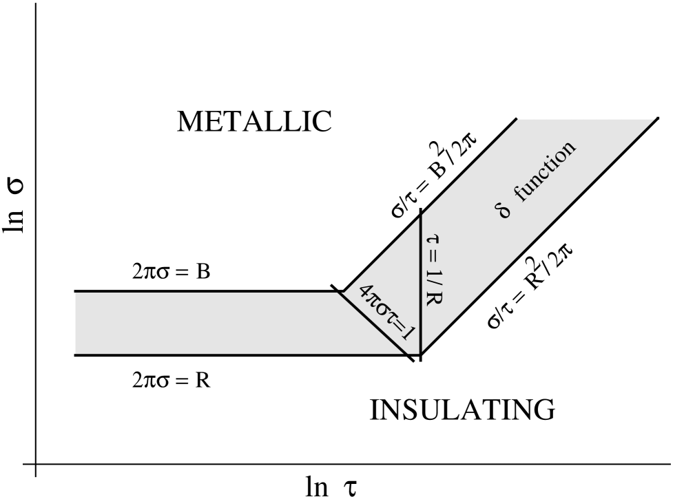
FIG. 1.: Schematic diagram to illustrate when ohmic losses are important for photoemission studies of cubic materials described by a Drude model. $\sigma_{0}$ is the DC conductivity and $\tau$ is the relaxation time. R is the resolution of the detector or the size of the smallest feature of interest. B is the bandwidth or the total energy range of interest. Ohmic losses are not important in either the metallic or insulating regime. They are potentially important in the shaded region in between these two limits. Within the shaded region the loss function can be characterized as follows. To the left of the $4\pi\sigma_{0}\tau$ line $P(\omega)$ is peaked about zero frequency. To the right it is peaked about $\omega_{0}=\sqrt{2\pi\sigma_{0}/\tau}$. To the right of the $\tau=1/R$ line $P(\omega)$ may be approximated by a delta function at $\omega_{0}$.

REFERENCES

- [1] K. Schulte, M.A. James, P.G. Steeneken, G.A. Sawatzky, R. Suryanarayanan, G. Dhalenne and A. Revcolevschi, Phys. Rev. B. 63, 165429 (2001).
- [2] R. Joynt, Science 284, 777 (1999).
- [3] D. Lynch and C.G. Olson Photoemission Studies of High-temperature Superconductors, (Cambridge Univ. Press, New York, 1999), p. 50ff.
- [4] D.L. Mills, Phys. Rev. B 62, 11197 (2000).
- [5] R. Haslinger and R. Joynt, J. Elect. Spect. 117, 31 (2001).
- [6] H. Ibach and D. L. Mills Electron Energy Loss Spectroscopy and Surface Vibrations (Academic, San Francisco, 1982).
- [7] H. Ibach, Surface Science 299/300, 116 (1994) reviews this work.
- [8] H. Ibach, Phys. Rev. Lett. 24, 1416 (1970).
- [9] T. Ishikawa, K. Tobe, T. Kimura, T. Katsufuji and Y. Tokura, Phys. Rev. B. 62, 12354 (2000).