On the Occurrence of Finite-Time-Singularities in Epidemic Models of Rupture, Earthquakes and Starquakes

Abstract

We present a new kind of critical stochastic finite-time-singularity, relying on the interplay between long-memory and extreme fluctuations. We illustrate it on the well-established epidemic-type aftershock (ETAS) model for aftershocks, based solely on the most solidly documented stylized facts of seismicity (clustering in space and in time and power law Gutenberg-Richter distribution of earthquake energies). This theory accounts for the main observations (power law acceleration and discrete scale invariant structure) of critical rupture of heterogeneous materials, of the largest sequence of starquakes ever attributed to a neutron star as well as of earthquake sequences.

A large portion of the current work on rupture and earthquake prediction is based on the search for precursors to large events in the seismicity itself. Observations of the acceleration of seismic moment leading up to large events and “stress shadows” following them have been interpreted as evidence that seismic cycles represent the approach to and retreat from a critical state of a fault network Sorsammis . This “critical state” concept is fundamentally different from the long-time view of the crust as evolving spontaneously in a statistically stationary critical state, called self-organized criticality (SOC) BakTangSorSor . In the SOC view, all events belong to the same global population and participate in shaping the self-organized critical state. Large earthquakes are inherently unpredictable because a big earthquake is simply a small earthquake that did not stop. By contrast, in the critical point view, a great earthquake plays a special role and signals the end of a cycle on its fault network. The dynamical organization is not statistically stationary but evolves as the great earthquake becomes more probable. Predictability might then become possible by monitoring the approach of the fault network towards the critical state. This hypothesis first proposed in Sorsammis is the theoretical induction of a series of observations of accelerated seismicity SykesJaum1 ; BufeVarnes which has been later strengthened by several other observations HarrisSimpson ; Bowmanetal ; Zoller ; Yin . Theoretical support has also come from simple computer models of critical rupture critrupd and experiments of material rupture expcrit , cellular automata, with Anghel and without Huang long-range interaction, and from granular simulators Mora . Models of regional seismicity with more faithful fault geometry have been developed that also show accelerating seismicity before large model events Heibenkin ; BK ; benzion .

There are at least five different mechanisms that are known to lead to critical accelerated seismicity of the form

$$N(t)\propto 1/(t_{c}-t)^{m}$$ (1)

ending at the critical time $t_{c}$, where $N(t)$ is the seismicity rate (or acoustic emission rate for material rupture). Such finite-time-singularities are quite common and have been found in many well-established models of natural systems, either at special points in space such as in the Euler equations of inviscid fluids, in vortex collapse of systems of point vortices, in the equations of General Relativity coupled to a mass field leading to the formation of black holes, in models of micro-organisms aggregating to form fruiting bodies, or in the more prosaic rotating coin (Euler’s disk). They all involve some kind of positive feedback, which in the rupture context can be the following (see SamsorPNAS for a review): sub-critical crack growth DasScholz , geometrical feedback in creep rupture Krajcinovic , feedback of damage on the elastic coefficients with strain dependent damage rate benzion , feedback in a percolation model of regional seismicity SamsorPNAS , feedback in a stress-shadow model for regional seismicity BK ; SamsorPNAS .

While these mechanisms are plausible, their relevance to the earth crust remains unproven. Here, we present a novel mechanism leading to a new kind of critical stochastic finite-time-singularity in the seismicity rate, using the well-established epidemic-type aftershock sequence (ETAS) model for aftershocks, introduced by KK ; Ogata1 , based solely on the most solidly documented stylized facts of seismicity mentioned above. The adjective “stochastic” emphasizes the fact that the critical time $t_{c}$ is determined in large part by the specific sets of innovations of the random process. We show that, in a finite domain of its parameter space, the rate of seimic activity in the ETAS model diverges in finite time according to (1). The underlying mechanism relies on large deviations occuring in an explosive branching process. One of the advantage of this discovery is to be able to account for the observations of accelerated seismicity and acoustic emission in material failure, without invoking any new ingredient other than those already well-established empirically. We apply this insight to quantify the longest available starquake sequence of a neutron star soft $\gamma$-ray repeaters.

We shall use the example of earthquakes but the model applies similarly to microcracking in materials. The ETAS model is a generalization of the modified Omori law, in that it takes into account the secondary aftershock sequences triggered by all events. The modified Omori’s law states that the occurrence rate of the direct aftershock-daughters from an earthquake decreases with the time from the mainshock according to the “bare propagator” $K/{(t+c)}^{p}$. In the ETAS model, all earthquakes are simultaneously mainshocks, aftershocks and possibly foreshocks. Contrary to the usual definition of aftershocks, the ETAS model does not impose an aftershock to have an energy smaller than the mainshock. This way, the same law describes both foreshocks, aftershocks and mainshocks. An observed “aftershock” sequence of a given earthquake (starting the clock) is the result of the activity of all events triggering events triggering themselves other events, and so on, taken together. The corresponding seismicity rate (the “dressed propagator”), which is given by the superposition of the aftershock sequences of all events, is the quantity we derive here.

Each earthquake (the “mother”) of energy $E_{i}\geq E_{0}$ occurring at time $t_{i}$ gives birth to other events (“daughters”) of any possible energy, chosen with the Gutenberg-Richter density distribution $P(E)=\mu/(E/E_{0})^{1+\mu}$ with exponent $\mu\simeq 2/3$, at a later time between $t$ and $t+dt$ at the rate

$$\phi_{E_{i}}(t-t_{i})=\rho(E_{i})~{}\Psi(t-t_{i})~{}.$$ (2)

$\rho(E_{i})=K~{}(E_{i}/E_{0})^{a}$ gives the number of daughters born from a mother with energy $E_{i}$, with the same exponent $a$ for all earthquakes. This term accounts for the fact that large mothers have many more daughters than small mothers because the larger spatial extension of their rupture triggers a larger domain. $E_{0}$ is a lower bound energy below which no daughter is triggered. $\Psi(t-t_{i})={\theta~{}c^{\theta}\over(t-t_{i}+c)^{1+\theta}}$ is the normalized waiting time distribution (local Omori’s law or “bare propagator”) giving the rate of daughters born a time $t-t_{i}$ after the mother.

The ETAS model is fundamentally a “branching” model Branching with no “loops”, i.e., each event has a unique “mother-mainshock” and not several. This “mean-field” or random phase approximation allows us to simplify the analysis while still keeping the essential physics in a qualitative way. The problem is to calculate the “dressed” or “renormalized” propagator (rate of seismic activity) that includes the whole cascade of secondary sequences sorsor . The key parameter is the average number $n$ (or “branching ratio”) of daughter-earthquakes created per mother-event, summed over all possible energies. $n$ is equal to the integral of $\phi_{E_{i}}(t-t_{i})$ over all times after $t_{i}$ and over all energies $E_{i}\geq E_{0}$. This integral converges to a finite value $n<\infty$ for $\theta>0$ (local Omori’s law decay faster than $1/t$) and for $a<\mu$ (not too large a growth of the number of daughters as a function of the energy of the mother). The resulting average rate $N(t)$ of seismicity is the solution of the Master equation helmsor

$$N(t)=\int_{0}^{t}d\tau~{}N(\tau)\int_{E_{0}}^{E_{\rm max}(t)}dE^{\prime}~{}P(E^{\prime})~{}\phi_{E^{\prime}}(t-\tau)$$ (3)

giving the number $N(t)dt$ of events occurring between $t$ and $t+dt$ of any possible energy. We have made explicit the upper bound $E_{\rm max}(t)$ equal to the typical maximum earthquake energy sampled up to time $t$. For $a<\mu$, this upper bound has no impact on the results and can be replaced by $+\infty$ helmsor . There may be a source term $S(t)$ to add to the r.h.s. of (3), corresponding to either a constant background seismicity or to a large triggering earthquake. In this last case, the rate $N(t)$ solution of (3) is the “dressed” propagator giving the renormalized Omori’s law. A rich behavior, which has been fully classified by a complete analytical treatment helmsor , has been found: sub-criticality $n<1$ sorsor and super-criticality $n>1$ helmsor , where $n$ depends on the control parameters $\mu$, $a$, $\theta$, $K$ and $c$. With a single value of the exponent $1+\theta$ of the “bare” propagator $\Psi(t)\sim 1/t^{1+\theta}$, we obtain a continuum of apparent exponents for the global rate of aftershocks helmsor which may account for the observed variability of Omori’s exponent $p$ around $p=1$ reported by many workers.

Here, we explore the regime $a\geq\mu$, for which $n$ is infinite. This signals the impact of large earthquake energies, suggesting the relevance of the upper bound $E_{\rm max}(t)$ in (3). This case is actually observed in real seismicity by Drakatos who obtained $a>\mu$ for some aftershock sequences in Greece, and by guoogata who found $a>\mu$ for 13 out of 34 aftershock sequences in Japan. This case $a>\mu$ also characterizes the seismic activity preceding the 1984 $M=6.8$ Nagano Prefecture earthquake Ogata2 . After the mainshock, the seismicity returned in the sub-critical regime $\theta>0$, $a<\mu$ and $n<1$.

This case $a\geq\mu$ is similar to that found underlying various situations of anomalous transport BG : in this regime of large fluctuations, the integral over earthquake energies is dominated by the upper bound. The maximum energy $E_{\rm max}(t)$ sampled by $N(t)\Delta t$ earthquakes is given by the standard condition $N(t)\Delta t\int_{E_{0}}^{E_{\rm max}(t)}dE^{\prime}~{}P(E^{\prime})\approx 1$. This yields the robust median estimate $E_{\rm max}(t)\sim[N(t)\Delta t]^{1/\mu}$. Actually, $E_{\rm max}(t)$ is itself distributed according to the Gutenberg-Richter distribution and thus exhibits large fluctuations from realization to realization, as we can see in Fig. 1. Putting this estimation of $E_{\rm max}(t)$ in (3), we get

$$N(t)\propto\int_{0}^{t}d\tau~{}{N(\tau)\over(t-\tau+c)^{1+\theta}}~{}[N(\tau)\Delta\tau]^{(a-\mu)/\mu}~{}.$$ (4)

Let us note the appearance of the new term $[N(\tau)\Delta\tau]^{(a-\mu)/\mu}$ resulting from the contribution of the upper bound in the integral $\int dE^{\prime}P(E^{\prime})$. This term replaces the constant found for the case $a<\mu$. Equation (4) shows that the exploration of larger and larger events in the tail in the Gutenberg-Richer distribution transforms the linear Master equation (3) into a non-linear equation: the non-linearity expresses a positive feedback according to which the larger is the rate $N(t)$ of seismicity, the larger is the maximum sampled earthquake, and the larger is the number of daughters resulting from these extreme events. This process self-amplifies and leads to the announced finite-time singularity (1). However, to complete the derivation, we need to determine the yet unspecified time increment $\Delta\tau$. If $N(\tau)$ obeys (1), $\Delta\tau$ is not a constant that can be factorized away: it is determined by the condition that, over $\Delta\tau$, $N(\tau)$ does not change “significantly” in the interval $[\tau,\tau+\Delta\tau]$, i.e., no more than by a constant factor. Using the assumed power law solution (1), this gives $\Delta\tau\propto t_{c}-\tau$. Using this and inserting (1) into (4), we get,

$$m = {a/\mu\over(a/\mu)-1}~{},~{}~{}~{}~{}~{}~{}~{}~{}~{}~{}~{}~{}~{}~{}~{}~{}~{}~{}t_{c}-t\leq c$$

$$m = {(a/\mu)-1-\theta~{}H(-\theta)\over(a/\mu)-1}~{},~{}~{}~{}t_{c}-t\gg c~{},$$ (5)

where $H$ is the Heaviside function. Note that (5) predicts an exponent $m>1$ which is independent of $\theta$ close to the critical time $t_{c}$. This is due to the fact that the time decay of the Omori’s kernel is not felt for $t_{c}-t\leq c$, where $c$ acts as an ultraviolet cut-off. It is also interesting to find that $m=1$ independently of $a$ and $\theta$ in the regime $\theta>0$ (with of course $a>\mu$) for which Omori’s kernel $\sim 1/t^{1+\theta}$ decays sufficiently fast at long times that the predominant contributions to the present seismic rate come from events in the immediate past of the present time of observation. In constrast, the case $\theta<0$ is analogous to the anomalous long-time memory regime BG which keeps for ever the impact of past events on future rates.

This prediction, based on the careful analysis of the integral in (4), has been verified by direct numerical evaluation of the equation (4). We have also checked that numerical Monte Carlo simulations of the ETAS model generates catalogs of events following this prediction, in an ensemble or median sense. Figure 1 shows the cumulative number ${\cal N}(t)=\int_{0}^{t}d\tau~{}N(\tau)$ of events for a typical realization of the ETAS model and compares it with $E_{\rm max}(t)$ to illustrate that ${\cal N}(t)$ is mostly controlled by the sampling of $E_{\rm max}(t)$, as discussed in the derivation of expression (4) leading to the finite-time-singularity (1). For the value $\mu=1$ chosen here, $E_{\rm max}(t)$ follows the same power law as the cumulative number, as observed. The dashed line is the power law prediction (1) with (5) for $a/\mu=1.5$ and $\theta=-0.2$ with slope $m-1=0.4$. We have also generated 500 such catalogs and report in the inset the distribution $d(m)$ of exponents $m$ obtained by a best fit of ${\cal N}(t)$ for each of the 500 catalogs to a power law $1/(t_{c}-t)^{m-1}$. The median of $d(m)$ is exactly equal to the prediction shown by the vertical thin line while the mode is very close to it. Note however a rather large dispersion which is expected from the highly intermittent dynamics characteristic of this extreme-dominated dynamics. We now report a few comparisons between the prediction (5) and the median value of the exponent $m$ obtained from 500 simulations for the following parameters: $\theta=-0.2$, $a=1.7,\mu=1$, predicted $m=1.29$, median $m=1.37$; $\theta=-0.2$, $a=1.3,\mu=1$, predicted $m=1.67$, median $m=1.61$; $\theta=-0.1$, $a=1.5,\mu=1$, predicted $m=1.20$, median $m=1.29$; $\theta=-0.3$, $a=1.5,\mu=1$, predicted $m=1.60$, median $m=1.62$. For $a>1.8\mu$, the fluctuations are so large that a reliable determination of the median becomes questionable from a sample of 500 realizations and many more would be needed.

Figure 1 shows that the power law singularities are decorated by quite strong steps or oscillations, approximately equidistant in the variable $\ln(t_{c}-t)$. This log-periodicity has been previously proposed as a possibly important signature of rupture and earthquake sequences approaching a critical point Sorsammis ; expcrit . Here, we present a simple novel mechanism for this observation, based on a refinement of the previous argument leading to $E_{\rm max}(t)\sim[N(t)\Delta t]^{1/\mu}$. Indeed, the most probable value for the energy $E_{n}$ of the $n$-th largest earthquake ranked from the largest $E_{1}=E_{\rm max}$ to the smallest one is given by $E_{n}(t)=\{[{\cal N}(t)\mu+1]/[n\mu+1]\}^{1/\mu}$ rank , where ${\cal N}(t)=\int_{0}^{t}N(t^{\prime})dt^{\prime}$. Let us assume that the last new record was broken at time $t_{1}$ leading to $E_{1}(t_{1})=\{[{\cal N}(t_{1})\mu+1]/[\mu+1]\}^{1/\mu}$. The next record will occur at a time $t_{2}>t_{1}$ whose typical value is such that $E_{2}(t_{2})=E_{1}(t_{1})$ (the last record $E_{1}(t_{1})$ becomes the second largest event $E_{2}(t_{2})$ when a new record $E_{1}(t_{2})$ occurs). For large ${\cal N}(t)$, this gives ${{\cal N}(t_{2})\over{\cal N}(t_{1})}=(2\mu+1)/(\mu+1)$. The prefered scaling ratio of the average log-periodicity is $\lambda\equiv(t_{c}-t_{1})/(t_{c}-t_{2})=[(2\mu+1)/(\mu+1)]^{1/(m-1)}$. For $a/\mu=1.5,\theta=-0.2,m=1.4$ corresponding to figure 1, we obtain $\lambda\approx 2.3$, which is compatible with the data.

The prediction (5) rationalizes the “inverse” Omori’s law close to $1/(t_{c}-t)$ that has been documented for earthquake forshocks KKpred . The prediction (5) as well as the log-periodicity offers a general framework to rationalize several previous experimental reports of precursory acoustic emissions rates prior to global failures expcrit . In this case, the energy release rate $e(t)$ is found to follow a power law finite-time singularity. According to our theory, $e(t)\propto N(t)E_{\rm max}(t)\propto 1/(t_{c}-t)^{m+(m-1)/\mu}$.

Finally, we also show that this could explain starquakes catalogs. Starquakes are assumed to be ruptures of a super-dense $1$-km thick crust made of heavy nuclei stressed by super-strong stellar magnetic field. They are observed through the associated flashes of soft $\gamma$-rays radiated during the rupture. Starquakes exhibit all the main stylized facts of their earthly siblings Kosso . The thick line in figure 1 shows the cumulative number of starquakes of the SGR1806-20 sequence, which is the longest sequence (of 111 events) ever attributed to the same neutron star, as a function of the logarithm of the time $t_{c}-t$ to failure. The starquake data is compatible with $\mu=1$ Kosso , $a=1.5$ and $\theta=-0.2$, leading to $m=1.4$.

We are grateful to V. Keilis-Borok and V. Kossobokov for sharing the starquake data with us and W.-X. Zhou for discussions and help in a preliminary analysis of the data.

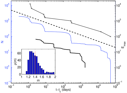
Figure 1: Cumulative number of events (scale on the left) as a function of the time from the critical point $t_{c}$ for the starquake sequence (solid black line) and one typical simulation of the ETAS model (solid thin line) generated with $\theta=-0.2$, $a/\mu=1.5$ and $c=0.001$. For the starquakes, $t_{c}$ is the time of the strongest observed starquake in the sequence. The dashed line shows the theoretical exponent $m-1=0.4$ (5) for $t_{c}-t>c$. The crosses $\times$ joined by straight segments give the time evolution of $E_{\rm max}(t)$ (scale on the right). The inset gives the distribution of exponent measured for 500 numerical simulations. The median (vertical line) of the distribution of $m$-values is equal to the theoretical exponent $m=1.4$ (formula (5)).

References

- (1) Sornette, D. and Sammis, C.G., J. Phys. I France 5, 607 (1995); J. Geophys. Res. 101, 17661 (1996).
- (2) Sornette, A. and Sornette, D., Europhys. Lett. 9, 197 (1989); Bak, P. and Tang, C., J. Geophys. Res. 94, 15,635 (1989).
- (3) Sykes L.R. and S. Jaumé, Nature 348, 595 (1990).
- (4) Bufe C.G. and D.J. Varnes, J. Geophys. Res. 98, 9871 (1993).
- (5) Harris, R.A., and R.W. Simpson, Geophysical Res. Lett. 23, 229 (1996); Knopoff et al., J. Geophys. Res. 101, 5779 (1996); Jones, L. M., and E. Hauksson, Geophys. Res. Lett. 24, 469 (1997).
- (6) Bowman, D.D., et al., J. Geophys. Res. 103, 24359 (1998); Brehm, D.J. and Braile, L.W., Bull. Seism. Soc. Am. 88, 564 (1998); Jaumé, S.C. and L.R. Sykes, Pure Appl. Geophys. 155, 279 (1999); Ouillon, G. and Sornette, D., Geophys. J. Int. 143, 454 (2000).
- (7) Zoller, G., S. Hainzl, and J. Kurths, J. Geophys. Res., 106, 2167 (2001).
- (8) Yin, X-C., preprint (2001).
- (9) Sornette, D. and C. Vanneste, Phys. Rev. Lett. 68, 612 (1992); C. Vanneste and D. Sornette, J. Phys. I France 2 1621 (1992); D. Sornette , C. Vanneste and L. Knopoff, Phys. Rev. A 45, 8351 (1992); Sahimi. M. and S. Arbabi, Phys. Rev. Lett. 77, 3689 (1996); J.V. Andersen, D. Sornette and K.-T. Leung, Phys. Rev. Lett. 78, 2140 (1997).
- (10) Anifrani, J.-C., C. Le Floc’h, D. Sornette and B. Souillard, J. Phys. I France 5, 631 (1995); Lamaignère, L., F. Carmona and D. Sornette, Phys. Rev. Lett. 77, 2738 (1996); Garcimartin, A., Guarino, A., Bellon, L. and Ciliberto, S., Phys. Rev. Lett. 79, 3202-3205 (1997); Johansen, A. and D. Sornette, Eur. Phys. J. B 18, 163 (2000).
- (11) Anghel, M. et al., EOS Trans. Am.Geophys. Union 80, F923 (1999); preprint cond-mat/0002459; Sá Martins, J.C. et al., preprint cond-mat/0101343.
- (12) Huang, Y. et al., Europhys. Lett. 41, 43 (1998); Sammis, C.G. and S.W. Smith, Pure Appl. Geophys. 155, 307 (1999).
- (13) Mora, P. et al., in “Geocomplexity and the Physics of Earthquakes”, eds Rundle, J. B., Turcotte, D. L. & Klein, W. (Am. Geophys. Union, Washington, 2000); Mora, P. and D. Place, Pure Appl. Geophys., in press.
- (14) Heimpel, M., Nature 388, 865 (1997).
- (15) Bowman, D.D. and King, G.C.P., Geophys. Res. Lett. 28, 4039 (2001).
- (16) Ben-Zion, Y. and Lyakhovsky, V., submitted to Pure Appl. Geophys. (2001).
- (17) Sammis, S.G. and D. Sornette, Proc. Nat. Acad. Sci. USA, in press (2001) (cond-mat/0107143)
- (18) Das, S. and Scholz, C.H., J. Geophys. Res. 86, 6039 (1981).
- (19) Krajcinovic, D., Damage mechanics (North-Holland Series in Applied Mathematics and Mechanics, Elsevier, Amsterdam, 1996).
- (20) Kagan, Y.Y. and L. Knopoff, J. Geophys. Res. 86, 2853 (1981); Science 236, 1563 (1987).
- (21) Ogata, Y., J. Am. Stat. Assoc. 83, 9 (1988).
- (22) Ogata, Y., Tectonophysics 169, 159 (1989).
- (23) Guo, Z. and Y. Ogata, J. Geophys. Res. 102, 2857 (1997).
- (24) Vere-Jones, D., Mathematical Geology 9, 455 (1977).
- (25) Sornette, A. and D. Sornette, Geophys. Res. Lett. 6, 1981 (1999).
- (26) Helmstetter, A. and D. Sornette, J. Geophys. Res., 107, 2237, doi:10.1029/2001JB001580, 2002.
- (27) Drakatos, G. and J. Latoussakis, Journal of Seismology 5, 137 (2001).
- (28) Bouchaud, J.-P. and Georges, A., Phys. Rep. 195, 127 (1990); Sornette, D., Critical Phenomena in Natural Sciences (Springer Series in Synergetics, Heidelberg, 2000).
- (29) Jones, L. and P. Molnar, Nature 262, 677 (1976) Kagan, Y.Y. and L. Knopoff, Geophys. J. Roy. Astron. Soc. 55, 67- (1978); Jones, L.M. and P. Molnar, J. Geophys. Res. 84, 3596 (1979).
- (30) Kossobokov, V.G., Keilis-Borok, V.I. and Cheng, B.L., Phys. Rev. 61 N4 PTA:3529-3533 (2000).
- (31) Sornette, D. et al., J. Geophys. Res. 101, 13883 (1996).