Multi-overlap simulations of spin glasses

Abstract

We present results of recent high-statistics Monte Carlo simulations of the Edwards-Anderson Ising spin-glass model in three and four dimensions. The study is based on a non-Boltzmann sampling technique, the multi-overlap algorithm which is specifically tailored for sampling rare-event states. We thus concentrate on those properties which are difficult to obtain with standard canonical Boltzmann sampling such as the free-energy barriers $F^{q}_{B}$ in the probability density $P_{\cal J}(q)$ of the Parisi overlap parameter $q$ and the behaviour of the tails of the disorder averaged density $P(q)=[P_{\cal J}(q)]_{\rm av}$.

1 Introduction

A widely studied class of spin-glass materials[1, 2, 3, 4] consists of dilute solutions of magnetic transition metal impurities in noble metal hosts, for instance[5] Au-2.98% Mn or[6] Cu-0.9% Mn, which is one of the best investigated metallic spin glasses. In these systems, the interaction between impurity moments is caused by the polarization of the surrounding Fermi sea of the host conduction electrons, leading to an effective interaction of the so-called RKKY form[7]

$$J_{\rm eff}(R)=\frac{\cos(2k_{F}R)}{R^{3}}\enspace,\qquad k_{F}R\gg 1\enspace,$$ (1)

where $k_{F}$ is the Fermi wave number. For an illustration, see Fig. 1. This constitutes the two basic ingredients necessary for spin-glass behaviour, namely

• randomness – in course of the dilution process the positions of the impurity moments are randomly distributed, and

• competing interactions – due to the oscillations in (1) as a function of the distance $R$ between the spins some of the interactions are positive and some are negative.

The competition among the different interactions between the moments means that no single configuration of spins is uniquely favoured by all of the interactions, a phenomenon which is commonly called “frustration”. This leads to a rugged free-energy landscape with probable regions (low free energy) separated by rare-event states (high free energy), illustrated in many previous articles by vague sketches similar to our Fig. 2. Experimentally this may be inferred from the phenomenon of aging which is typical of measurements of the remanent magnetization in the spin-glass phase[8].

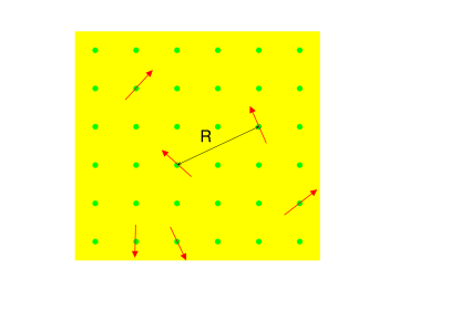
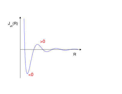
Figure 1: The two basic ingredients for spin-glass behaviour: Randomly distributed spin moments of transition metal impurities (e.g. Mn) in a noble metal host (e.g. Cu), and the characteristic oscillatory form of their effective RKKY interactions with competing positive (ferromagnetic) and negative (antiferromagnetic) regions.

However, despite the large amount of experimental, theoretical and simulational work done in the past thirty years to elucidate the spin-glass phase,[1, 2, 3, 4] the physical mechanisms underlying its peculiar properties are not yet fully understood. To cope with the enormous complexity of the problem various levels of simplified models have been studied theoretically. A simplified lattice model which reflects the two basic ingredients for spin-glass behaviour is the Edwards-Anderson[9] Ising (EAI) model defined through the energy

$$E=-\sum_{\langle ik\rangle}J_{ik}\,s_{i}s_{k}\ ,$$ (2)

where the fluctuating spins $s_{i}$ can take the values $\pm 1$. The coupling constants $J_{ik}$ are quenched, random variables taking positive and negative signs, thereby leading to competing interactions. In our study we worked with a bimodal distribution, $J_{ik}=\pm 1$ with equal probabilities, but other choices such as the Gaussian distribution, ${\cal P}(J_{ik})\propto\exp(-J_{ik}^{2}/2\Delta^{2})$ with $\Delta$ parameterizing its width, have also been considered, in particular in analytical work. In (2), the lattice sum runs over all nearest-neighbour pairs of a $d$-dimensional (hyper-) cubic lattice of size $N=L^{d}$ with periodic boundary conditions.

figure=Figures/sketch.eps,width=10cm

Figure 2: Typical sketch of the rugged free-energy landscape of spin glasses with many minima separated by rare-event barriers.

An analytically more tractable mean-field model, commonly known as the Sherrington-Kirkpatrick[10] (SK) model, emerges when each spin is allowed to interact with all others. Alternatively one may consider the mean-field treatment as an approximation which is expected to become accurate in high dimensions[11]. In physical dimensions, however, its status is still unclear and an alternative droplet approximation[12] has been proposed. The two treatments yield conflicting predictions which have prompted quite a controversial discussion over many years. Numerical approaches such as Monte Carlo (MC) simulations can, in principle, provide arbitrarily precise results in physical dimensions. In practice, however, the simulational approach is severely hampered by an extremely slow (pseudo-) dynamics of the stochastic process.

To overcome the slowing-down problem various novel simulation techniques have been devised in the past few years. While some of them only aim at improving the (pseudo-) dynamics of the MC process, others are in addition also well suited for a quantitative characterization of the free-energy barriers responsible for the slowing-down problem. Among the latter category is the multi-overlap algorithm[13] which has recently been employed in quite extensive MC simulations[14, 15, 16, 17] of the EAI spin-glass model in three and four dimensions. The purpose of this note is to give an overview of the recent progress achieved with this method.

2 Model Parameters and Simulation Method

As order parameter of the EAI model one usually takes the Parisi overlap parameter[11]

$$q=\frac{1}{N}\sum_{i=1}^{N}s^{(1)}_{i}\,s^{(2)}_{i}\ ,$$ (3)

where the spin superscripts label two independent (real) replicas for the same realization of randomly chosen exchange coupling constants ${\cal J}=\{J_{ik}\}$. For given ${\cal J}$ the probability density of $q$ is denoted by $P_{\cal J}(q)$, and thermodynamic expectation values are computed as $\langle\dots\rangle_{\cal J}\equiv\sum_{\{s\}}(\dots)\exp(-\beta H[{\cal J}])/\sum_{\{s\}}\exp(-\beta H[{\cal J}])$, where $\beta=1/k_{B}T$ is the inverse temperature in natural units. The freezing temperature is known to be at $\beta_{c}=0.90(3)$ in 3D (Ref. 18) and at $\beta_{c}=0.485(5)$ in 4D (Ref. 19), respectively.

On finite lattices the results necessarily depend on the randomly chosen quenched disorder. To get a better approximation of the infinite system (apart from special problems with so-called non-self-averaging), one performs averages over many hundreds or even thousands of (quenched) disorder realizations denoted by

$$P(q)=\left[P_{\cal J}(q)\right]_{\rm av}=\frac{1}{\#{\cal J}}\sum_{\cal J}P_{\cal J}(q)\ ,\qquad[\langle\dots\rangle_{\cal J}]_{\rm av}=\frac{1}{\#{\cal J}}\sum_{\cal J}\langle\dots\rangle_{\cal J}\ ,$$ (4)

where $\#{\cal J}$ ($\rightarrow\infty$) is the number of realizations considered. Below the freezing temperature, in the infinite-volume limit $N\rightarrow\infty$, a non-vanishing part of $P(q)$ between its two delta-function peaks at $\pm q_{\rm max}$ characterizes the mean-field picture[11] of spin glasses, whereas in ferromagnets as well as in the droplet picture[12] of spin glasses $P(q)$ exhibits only the two delta-function peaks. Most studies so far considered mainly the averaged quantities.

For a better understanding of the free-energy barriers sketched in Fig. 2, the probability densities for individual realizations ${\cal J}$ play the central role. It is, of course, impossible to get complete control over the full state space, and to give a well-defined meaning to “system state” (the $x$-axis in Fig. 2), one has to concentrate on one or a few characteristic properties. In our work we focused on the order parameter and thus those free-energy barriers $F_{B}^{q}$ which are reflected by the minima of $P_{\cal J}(q)$. A few typical shapes of $P_{\cal J}(q)$ as obtained in our simulations are shown in Fig. 3. Conventional, canonical MC simulations are not suited for such a study because the likelihood to generate the corresponding rare-event configurations in the Gibbs canonical ensemble is very small. This problem is overcome by non-Boltzmann sampling[20, 21] with the multi-overlap weight[13]

$$w_{\cal J}(q)=\exp\left[\beta\sum_{\langle ik\rangle}J_{ik}\left(s_{i}^{(1)}s_{k}^{(1)}+s_{i}^{(2)}s_{k}^{(2)}\right)+S_{\cal J}(q)\right]\ ,$$ (5)

where the two replicas are coupled by $S_{\cal J}(q)$ in such a way that a broad multi-overlap histogram $P_{\cal J}^{\rm muq}(q)$ over the entire accessible range $-1\leq q\leq 1$ is obtained, see Fig. 4. When simulating with the multi-overlap weight (5), canonical expectation values of any quantity $\cal O$ can be reconstructed by reweighting, $\langle{\cal O}\rangle_{\cal J}^{\rm can}=\langle{\cal O}e^{-S_{\cal J}}\rangle_{\cal J}/\langle e^{-S_{\cal J}}\rangle_{\cal J}$.

Figure 3: Typical probability densities $P_{\cal J}(q)$ as obtained in multi-overlap simulations of the 3D EAI spin-glass model on a $12^{3}$ lattice at $T=1\approx 0.88T_{c}$.

$$~{}~{}~{}~{}~{}P_{\cal J}^{\rm muq}(q)=P_{\cal J}^{\rm can}(q)\exp[{S_{\cal J}(q)}]$$

Figure 4: Illustration of the relation between canonical densities $P_{\cal J}^{\rm can}(q)$ depicted in Fig. 3 and ideally flat multi-overlap densities $P_{\cal J}^{\rm muq}(q)$.

The multi-overlap algorithm may be summarized as follows:

• An iterative construction of the weight function $W_{\cal J}(q)\equiv\exp(S_{\cal J}(q))$, for each of the quenched disorder realizations separately.

• An equilibration period with fixed weight function.

• The production run with fixed weight function.

Ideally $W_{\cal J}$ should satisfy $P_{\cal J}^{\rm muq}(q)=P^{\rm can}_{\cal J}(q)W_{\cal J}(q)={\rm const.}$, i.e., should give rise to a completely flat multi-overlap probability density $P_{\cal J}^{\rm muq}(q)$ as sketched in Fig. 4. Of course, $P^{\rm can}_{\cal J}(q)$ is a priori unknown and one has to proceed by iteration. Let us thus assume some approximate $W_{{\cal J},n}$ is given. The simulation would then yield $P_{{\cal J},n}^{\rm muq}$ which, in general, is not yet perfectly flat. If $P_{{\cal J},n}^{\rm muq}$ was sampled with arbitrary precision, the desired weight function would be $W_{\cal J}\propto W_{{\cal J},n}/P_{{\cal J},n}^{\rm muq}$. For the update procedure we are actually only interested in relative transition amplitudes and it is therefore useful to rephrase the iteration in terms of

$$R_{\cal J}(q)\equiv W_{\cal J}(q+\Delta q)/W_{\cal J}(q)=R_{{\cal J},n}(q)P_{{\cal J},n}^{\rm muq}(q)/P_{{\cal J},n}^{\rm muq}(q+\Delta q)\ ,$$ (6)

where $\Delta q=2/N$ is the step-width in $q$ as defined in Eq. (3). When updating the spins in the nth iteration, $R_{{\cal J},n}(q)=W_{{\cal J},n}(q+\Delta q)/W_{{\cal J},n}(q)$ has to be considered as a given, fixed function of $q$. The multi-overlap histogram $P_{{\cal J},n}^{\rm muq}(q)$, however, is always a noisy estimator whose statistical errors can be estimated by $\sqrt{P_{{\cal J},n}^{\rm muq}(q)}$ (neglecting auto- and cross-correlations and assuming unnormalized histograms counting the number of hits). By taking the logarithm in Eq. (6) it is then straightforward to obtain the squared error on $\ln R_{\cal J}(q)$,

$$\epsilon^{2}_{\ln R_{\cal J}(q)}\equiv 1/p(q)=1/P_{{\cal J},n}^{\rm muq}(q)+1/P_{{\cal J},n}^{\rm muq}(q+\Delta q)\ .$$ (7)

We now have two noisy estimators, $R_{{\cal J}}(q)$ and $R_{{\cal J},n}(q)$ (with squared inverse errors $p(q)$ and $p_{n}(q)$), which may be linearly combined to yield an optimized estimator $\ln R_{{\cal J},n+1}(q)=\kappa_{n}(q)\ln R_{\cal J}(q)+[1-\kappa_{n}(q)]\ln R_{{\cal J},n}(q)$, with

$$\kappa_{n}(q)=p(q)/[p(q)+p_{n}(q)]\ ,$$ (8)

such that the statistical error of the linear combination is minimized. By exponentiating the optimized estimator and using Eq. (6), we finally arrive at the recursion

$$R_{{\cal J},n+1}(q) = R_{\cal J}(q)^{\kappa_{n}(q)}R_{{\cal J},n}(q)^{1-\kappa_{n}(q)}$$ (9)

$$= R_{{\cal J},n}(q)\left[P_{{\cal J},n}^{\rm muq}(q)/P_{{\cal J},n}^{\rm muq}(q+\Delta q)\right]^{\kappa_{n}(q)},$$

$$p_{n+1}(q) = p(q)+p_{n}(q)\ .$$ (10)

Once $W_{\cal J}(q)=\exp(S_{\cal J}(q))$ is determined and kept fixed, the system is equilibrated and the data production can be performed.

We measure the (pseudo-) dynamics of the multi-overlap algorithm in terms of the autocorrelation time $\tau_{\cal J}^{\rm muq}$ which is defined by counting the average number of sweeps it takes to complete the cycle $q=0\to|q|=1\to 0$. Adopting the usual terminology[20, 21] for a first-order phase transition, we shall call such a cycle a “tunnelling” event. The weight iteration was stopped after at least 10 “tunnelling” events occurred, and in the production runs we collected at least 20 “tunnelling” events. To allow for standard reweighting in temperature we stored besides $P_{\cal J}(q)$ and the time series of $q$ also the energies and magnetizations of the two replicas. The number of sweeps between measurements was adjusted by an adaptive data compression routine to ensure that each time series consists of $2^{16}=65\,536$ measurements separated by approximately $\tau_{\cal J}^{\rm muq}$ sweeps.

3 Results

Due to the large number of realizations to be simulated, the final results are relatively costly. The studied cases are summarized in Table 1, where also the simulation temperatures are given: $T=1\approx 0.88T_{c}$ and $T=1.14\approx T_{c}$ in 3D, and $T=1/0.6\approx 0.85T_{c}$ in 4D. The $J_{ik}$ realizations were drawn using the pseudo random number generators RANMAR [22] and RANLUX [23, 24] (luxury level 4). For the spin updates we always employed the faster RANMAR generator.

	3D		4D
$L$	$T=1.00$	$T=1.14$	$T=1/0.6$
4	8 192	8 192	4 096
6	8 192	8 192	4 096
8	8 192	8 192	1 024
12	640	1 024
16		256

Table 1: Number of simulated realizations #$\cal J$.

By fitting the averaged autocorrelation times to the power-law ansatz $\ln([\tau_{\cal J}^{\rm muq}]_{\rm av})=a+z\,\ln(N)$, we obtained[15] $z=2.32(7)$ and $z=1.94(2)$ in the 3D and 4D spin-glass phase, respectively. Even though the quality of the fits is quite poor and an exponential behaviour can hardly be excluded, they clearly show that the slowing down is quite off from the theoretical optimum $z=1$ one would expect if the multi-overlap autocorrelation time $\tau_{\cal J}^{\rm muq}$ is dominated by a random-walk behaviour between $q=-1$ and $+1$. In multicanonical simulations of the 3D model with broad energy histograms an even larger exponent of $z=2.8(1)$ has been observed[25]. The large values of $z$ suggest that the canonical overlap barriers are not the exclusive cause for the slowing down of spin-glass dynamics below the freezing point, i.e., the projection of the multi-dimensional state space onto the $q$-direction hides important features of the free-energy landscape of the model.

3.1 Free-Energy Barriers $F_{B}^{q}$

To define effective free-energy barriers $F_{B}^{q}$ we first construct an auxiliary 1D Metropolis-Markov chain[26] which has the canonical $P_{\cal J}(q)$ probability density as its equilibrium distribution. The tridiagonal transition matrix

$$T=\left(\begin{array}[]{cccc}1-w_{2,1}&w_{1,2}&0&\ldots\cr w_{2,1}&1-w_{1,2}-w_{3,2}&w_{2,3}&\ldots\cr 0&w_{3,2}&1-w_{2,3}-w_{4,3}&\ldots\cr 0&0&w_{4,3}&\ldots\cr\vdots&\vdots&\vdots&\ddots\cr\end{array}\right)\$$ (11)

is given in terms of the probabilities $w_{i,j}=\frac{1}{2}\min\Bigl{(}1,P_{\cal J}(q_{i})/P_{\cal J}(q_{j})\Bigr{)}$ ($i\neq j)$ for jumps from state $q=q_{j}$ to $q=q_{i}=i/N$ in steps of $\Delta q=\pm 2/N$ or 0. Since $T$ fulfills the detailed balance condition (with $P_{\cal J}$) it has only real eigenvalues. The largest eigenvalue $\lambda_{0}$ equals unity and is non-degenerate. The second largest eigenvalue $\lambda_{1}$ determines the autocorrelation time of the chain (in units of sweeps),

$$\tau_{B}^{q}=-\frac{1}{N\ln\lambda_{1}}\approx\frac{1}{N(1-\lambda_{1})}\ ,$$ (12)

which we use to define the associated effective free-energy barrier in the overlap parameter $q$ as

$$F_{B}^{q}\equiv\ln(\tau_{B}^{q})\ .$$ (13)

Our finite-size scaling (FSS) analyses of the thus defined overlap barriers are based on the (cumulative) distribution function $F(x)$. More precisely, we constructed[27] a peaked distribution function $F_{Q}(x)$ by reflecting $F(x)$ at its median value 0.5,

$$F_{Q}(x)\equiv\left\{\begin{array}[]{ll}F(x)&\quad{\rm for}\ F(x)\leq 0.5\ ,\\ 1-F(x)&\quad{\rm for}\ F(x)\geq 0.5\ .\\ \end{array}\right.$$ (14)

For self-averaging data the function $F_{Q}$ collapses in the infinite-volume limit to $F_{Q}(x)=0.5\ {\rm for}\ x=[x]_{\rm av}$ and 0 otherwise. For non-self-averaging quantities the width of $F_{Q}$ stays finite. The concept carries over to quantities which diverge in the infinite-volume limit, when for each lattice size scaled variables $x/x_{\rm med}$ are used, where $x_{\rm med}$ denotes the median defined through $F(x_{\rm med})=F_{Q}(x_{\rm med})=0.5$.

The behaviour of $F_{Q}(F_{B}^{q}/F^{q}_{B_{\rm med}})$ shown on the l.h.s. of Fig. 5 for the 3D case at $T=1$ clearly suggests that $F^{q}_{B}$ is a non-self-averaging quantity. In 4D the evidence is even stronger than in 3D. Non-self-averaging was also observed[15] for the autocorrelation times $\tau_{\cal J}^{\rm muq}$ of our algorithm while the energy is an example for a self-averaging quantity; cf. the r.h.s. of Fig. 5. For non-self-averaging quantities one has to investigate many samples and should report the FSS behaviour for fixed values of the cumulative distribution function $F$.

figure=Figures/FqB_3d.eps,width=6.3cm figure=Figures/FqE_3d.eps,width=6.3cm

Figure 5: Distribution function $F_{Q}$ (14) for the 3D overlap barriers (13) (left) and the energy (right) in the spin-glass phase at $T=1$ in units of their median values.

figure=Figures/3d_expfits.eps,width=6.4cm figure=Figures/3d_powfits.eps,width=6.4cm

Figure 6: FSS fits of the 3D overlap barriers $F_{B}^{q}$ in the spin-glass phase at $T=1$ for fixed values of the distribution function, $F=i/16$, $i=1,\dots,15$ (from bottom to top). Shown are the results for the mean-field prediction (15) (left) and the logarithmic ansatz (16) (right).

In Ref. 15 we performed FSS fits for $F=i/16$, $i=1,\dots,15$, assuming an ansatz suggested by mean-field theory[28, 29],

$$F_{B}^{q}=a_{1}+a_{2}\,N^{1/3}\ ,$$ (15)

corresponding to $\tau_{B}^{q}\propto e^{a_{2}\,N^{1/3}}$. In both dimensions the goodness-of-fit parameter[30] $Q$ turned out to be unacceptably small. The 3D fits are depicted on the l.h.s. of Fig. 6. We therefore also tried fits to the ansatz

$$F_{B}^{q}=\ln(c)+\alpha\,\ln(N)\ ,$$ (16)

corresponding to $\tau_{B}^{q}\propto N^{\alpha}$; cf. the r.h.s. of Fig. 6. Since in 3D as well as in 4D the average $Q$-value is now within the statistical expectation, the latter ansatz (16) is strongly favoured over the mean-field prediction (15). As a function of $F$ ($=1/16$ – $15/16$) the exponent $\alpha=\alpha(F)$ in the power law (16) varies smoothly from 0.8 to 1.1 in 3D and from 0.8 to 1.3 in 4D. A similar analysis[15] for the autocorrelation times $\tau_{\cal J}^{\rm muq}$ of the multi-overlap algorithm gives exponents $\alpha(F)$ which are larger, $\alpha^{\rm muq}(F)\approx\alpha^{q}_{B}(F)+1$. This is in agreement with our observation that other relevant barriers exist, which cannot be detected in the overlap parameter $q$.

3.2 Averaged Probability Densities $P(q)$

The averaged canonical densities $P(q)$ of the 3D model are shown in Fig. 7 for both $T=1\approx 0.88T_{c}$ and $T=1.14\approx T_{c}$. At least close to $T_{c}$ one expects that, up to finite-size corrections, the probability densities scale with system size. A method to confirm this visually is to plot $P^{\prime}(q)\equiv\sigma P(q)$ versus $q^{\prime}=q/\sigma$, where $\sigma$ is the standard deviation. By fitting the standard deviation to the expected FSS form $\sigma=c_{1}L^{-\beta/\nu}$ we obtained[17],

$$\frac{\beta}{\nu} = 0.312(4)\ ,\ \,Q=0.32\ {\rm~{}for}\ T=1.14\,,~{}~{}{\rm and}$$ (17)

$$\frac{\beta}{\nu} = 0.230(4)\ ,\ \,Q=0.99\ {\rm~{}for}\ T=1\,.$$ (18)

On the l.h.s. of Fig. 8 we show the scaling plot[17] for $T=1.14$ which demonstrates that the five probability densities collapse onto a single master curve.

figure=Figures/Pq_allboth_b100_full_p3.eps,width=6.25cm figure=Figures/Pq3d_EAITc.eps,width=6.65cm

Figure 7: Overlap probability densities for the 3D EAI model in the spin-glass phase (left) and close to criticality (right).

3.3 Tails of $P(q)$

The multi-overlap algorithm becomes particularly powerful when studying the tails of the probability densities which are highly suppressed compared to the peak values; see the r.h.s. of Fig. 8 which shows $P(q)$ at $T=1.14$ over more than 150 orders of magnitude. Based on the replica mean-field approach,  theoretical  predictions  for the scaling behaviour of the tails have been derived by Parisi and collaborators[31]. They showed that $P(q)=P_{\max}\,f(N\,(q-q_{\max}^{\infty})^{x})$ for $q>q_{\max}^{\infty}$ and concluded more quantitatively that

$$P(q)\sim\exp\left[-c_{1}\,N\,(q-q_{\max}^{\infty})^{x}\right]~{}~{}{\rm for}~{}~{}N\,(q-q_{\max}^{\infty})^{x}~{}~{}{\rm large}\ ,$$ (19)

with a mean-field exponent of $x=3$. By allowing for an overall normalization factor $c_{0}^{(N)}$ and taking the logarithm twice we have performed fits of the form[32, 33]

$$Y\equiv\ln\left[-\ln(P/c_{0}^{(N)})\right]-\ln N=\ln c_{1}+x\,\ln(q-q_{\max}^{\infty})\ .$$ (20)

Leaving the exponent $x$ as a free parameter, we arrived at the estimates $x=12(2)$ in 3D at $T=1$ and $x=5.3(3)$ in 4D at $T=1/0.6$ which are both much larger than the mean-field value of $x=3$.

By looking for reasonable alternatives we realized that for many other systems the statistics of extremes as pioneered by Fréchet, Fisher and Tippert, and von Mises[34, 35] has let to a good ansatz with universal properties[36, 37]. It is based on a standard result[34, 35], due to Fisher and Tippert, Kawata, and Smirnow, for the universal distribution of the first, second, third, $\dots$ smallest of a set of $N$ independent identically distributed random numbers. For an appropriate, exponential decay of the random number distribution their probability densities are given by the Gumbel form

$$f_{a}(x)\ =\ C_{a}\,\exp\left[\,a\,\left(x-e^{x}\,\right)\right]\ ,$$ (21)

in the limit of large $N$. The exponent $a$ takes the values $a=1,2,3,\dots$, corresponding, respectively, to the first, second, third, $\dots$ smallest random number of the set, $x$ is a scaling variable which shifts the maximum value of the probability density to zero, and $C_{a}$ is a normalization constant. For certain spin-glass systems the possible relevance of this universal distribution has been pointed out by Bouchaud and Mézard[38], and for instance also in applications to the 2D XY model in the spin-wave approximation[36, 37] the Gumbel ansatz (21) fitted well, albeit with a modified value of $a=\pi/2$.

In our case we set $x=b(q^{\prime}-q^{\prime}_{\rm max})$ and modified the first $x$ on the r.h.s. of (21) to $c\tanh(x/c)$, where $c>0$ is a constant, in order to reproduce the flattening of the densities towards $q^{\prime}=0$. Notice that in the tails of the densities, i.e. for large, positive $x$, this term is anyway subleading. A symmetric expression for $P^{\prime}(q^{\prime})$ reflecting its $q^{\prime}\to-q^{\prime}$ invariance is obtained by multiplying the above construction with its reflection about the $q^{\prime}=0$ axis,

$$P^{\prime}(q^{\prime})=C\exp\left\{a\left[c\tanh\left(\frac{b}{c}\,(q^{\prime}-q^{\prime}_{\max})\right)-e^{+b\,(q^{\prime}-q^{\prime}_{\max})}\right]\right\}\times(q^{\prime}\to-q^{\prime})\ .$$ (22)

Of course, the important large-$x$ behaviour of Eq. (21) is not at all affected by our manipulations.

By fitting this ansatz to our 3D data we obtained final estimates of $a=0.448(40)$ for $T=1.14$ and $a=0.446(37)$ for $T=1$, respectively. For $T=1.14$ our best fit is already included on the l.h.s. of Fig. 8. We see a good consistency between the data and the fit over a remarkably wide range of $q^{\prime}$. Even more impressive is the excellent agreement in the tails of the densities. Taking the $T=1.14$, $L=16$ result at face value, we find[17] a very good fit over a remarkable range of $200/\ln(10)\approx 87$ orders of magnitude!

figure=Figures/Pp3d_EAITc.eps,width=6.5cm figure=Figures/Ppln3d_EAI.eps,width=6.5cm

Figure 8: Rescaled overlap probability densities for the EAI spin-glass model on $L^{3}$ lattices at the critical temperature on a linear (left) and expanded logarithmic (right) scale. In the lower part of the plots the deviation $P^{\prime}_{16}(q^{\prime})-P^{\prime}_{\rm fit}(q^{\prime})\pm\triangle P^{\prime}_{16}(q^{\prime})$ of some $L=16$ data from the modified Gumbel fit (22) is shown (with an unimportant offset added in order to fit inside the figure).

4 Summary and Conclusions

Employing non-Boltzmann sampling with the multi-overlap MC algorithm we have investigated the probability densities $P_{\cal J}(q)$ of the Parisi order parameter $q$. The free-energy barriers $F_{B}^{q}$ as defined in Eq. (13) turn out to be non-self-averaging. The logarithmic scaling ansatz (16) for the barriers at fixed values $F$ of their cumulative distribution function is found to be favoured over the mean-field ansatz (15). Further, relevant barriers are still reflected in the autocorrelations of the multi-overlap algorithm.

The averaged densities exhibit a pronounced FSS collapse onto a common master curve even in the spin-glass phase. For the scaling of their tails towards $q=\pm 1$ we find qualitative agreement with the decay law predicted by mean-field theory, but with an exponent $x$ that is, in particular in 3D, much larger than theoretically expected. A much better fit over more than 80 orders of magnitude is obtained in 3D by using a modified Gumbel ansatz, rooted in extreme order statistics[34, 35]. The detailed relationship between the EAI spin-glass model and extreme order statistics remains to be investigated, and it is certainly a challenge to extend the work of Bouchaud and Mézard[38] to the more involved scenarios of the replica theory.

References

- [1] K. Binder and A.P. Young, Spin glasses: Experimental facts, theoretical concepts and open questions, Rev. Mod. Phys. 56, 801 (1986).
- [2] M. Mézard, G. Parisi, and M.A. Virasoro, Spin Glass Theory and Beyond (World Scientific, Singapore, 1987).
- [3] K.H. Fischer and J.A. Hertz, Spin Glasses (University Press, Cambridge, 1991).
- [4] A.P. Young (ed.), Spin Glasses and Random Fields (World Scientific, Singapore, 1997).
- [5] C.A.M. Mulder, A.J. van Duyneveldt, and J.A. Mydosh, Frequency and field dependence of the ac susceptibility of the Au Mn spin-glass, Phys. Rev. B 25, 515 (1982).
- [6] C.A.M. Mulder, A.J. van Duyneveldt, and J.A. Mydosh, Susceptibility of the Cu Mn spin-glass: Frequency and field dependences, Phys. Rev. B 23, 1384 (1981).
- [7] M.A. Ruderman and C. Kittel, Indirect exchange coupling of nuclear magnetic moments by conduction electrons, Phys. Rev. 96, 99 (1954); T. Kasuya, A theory of metallic ferro and antiferromagnetism on Zerner’s model, Prog. Theor. Phys. 16, 45 (1956); K. Yosida, Magnetic properties of Cu-Mn alloys, Phys. Rev. 106, 893 (1957).
- [8] P. Granberg, P. Svedlindh, P. Nordblad, L. Lundgren, and H.S. Chen, Time decay of the saturated remanent magnetization in a metallic spin glass, Phys. Rev. B 35, 2075 (1987); E. Vincent, J. Hammann, M. Ocio, J.-P. Bouchaud, and L.F. Cugliandolo, Slow dynamics and aging in spin glasses, in: Complex Behaviour of Glassy Systems, ed. M. Rubi, Lecture Notes in Physics, Vol. 492 (Springer-Verlag, Berlin, 1997), pp. 184-219 [cond-mat/9607224], and references given therein.
- [9] S.F. Edwards and P.W. Anderson, Theory of spin glasses, J. Phys. F 5, 965 (1975).
- [10] D. Sherrington and S. Kirkpatrick, Solvable model of a spin-glass, Phys. Rev. Lett. 35, 1792 (1975).
- [11] G. Parisi, Infinite number of order parameters for spin glasses, Phys. Rev. Lett. 43, 1754 (1979).
- [12] D.S. Fisher and D.A. Huse, Equilibrium behavior of the spin-glass ordered phase, Phys. Rev. B 38, 386 (1988).
- [13] B.A. Berg and W. Janke, Multioverlap simulations of the 3D Edwards-Anderson Ising spin glass, Phys. Rev. Lett. 80, 4771 (1998).
- [14] W. Janke, B.A. Berg, and A. Billoire, Energy barriers of spin glasses from multi-overlap simulations, Ann. Phys. (Leipzig) 7, 544 (1998); Multi-overlap simulations of free-energy barriers in the 3D Edwards-Anderson Ising spin glass, Comp. Phys. Comm. 121-122, 176 (1999).
- [15] B.A. Berg, A. Billoire, and W. Janke, Spin-glass overlap barriers in three and four dimensions, Phys. Rev. B 61, 12143 (2000).
- [16] W. Janke, B.A. Berg, and A. Billoire, Exploring overlap barriers in spin glasses with Monte Carlo simulations, in: Multiscale Computational Methods in Chemistry and Physics, Proceedings of the NATO Advanced Research Workshop, Eilat, Israel, April 2000, eds. A. Brandt, J. Bernholc, and K. Binder (IOS Press, Amsterdam, 2001), p. 198.
- [17] B.A. Berg, A. Billoire, and W. Janke, Functional form of the Parisi overlap distribution for the three-dimensional Edwards-Anderson Ising spin glass, preprint cond-mat/0108034, submitted to Phys. Rev. E.
- [18] N. Kawashima and A.P. Young, Phase transition in the three-dimensional Ising spin glass, Phys. Rev. B 53, R484 (1996).
- [19] D. Badoni, J.C. Ciria, G. Parisi, F. Ritort, J. Pech, and J.J. Ruiz-Lorenzo, Numerical evidence of a critical line in the 4d Ising spin glass, Europhys. Lett. 21, 495 (1993).
- [20] B.A. Berg, Introduction to multicanonical Monte Carlo simulations, Fields Inst. Commun. 26, 1 (2000) [cond-mat/9909236].
- [21] W. Janke, Multicanonical Monte Carlo simulations, Physica A 254, 164 (1998).
- [22] G. Marsaglia, A. Zaman, and W.W. Tsang, Toward a universal random number generator, Stat. Prob. Lett. 9, 35 (1990).
- [23] M. Lüscher, A portable high-quality random number generator for lattice field theory simulations, Comp. Phys. Comm. 79, 100 (1994).
- [24] F. James, RANLUX: A FORTRAN implementation of the high-quality pseudorandom number generator of Lüscher, Comp. Phys. Comm. 79, 111 (1994).
- [25] B.A. Berg, U.E. Hansmann, and T. Celik, Ground-state properties of the three-dimensional Ising spin glass, Phys. Rev. B 50, 16444 (1994).
- [26] N. Metropolis, A.W. Rosenbluth, M.N. Rosenbluth, A.H. Teller, and E. Teller, Equation of state calculations by fast computing machines, J. Chem. Phys. 21, 1087 (1953).
- [27] B.A. Berg, Introduction to Monte Carlo Simulations and Their Statistical Analysis, in preparation.
- [28] N.D. Mackenzie and A.P. Young, Lack of ergodicity in the infinite-range Ising spin-glass, Phys. Rev. Lett. 49, 301 (1982); Statics and dynamics of the infinite range Ising spin glass model, J. Phys. C 16, 5321 (1983); K. Nemoto, Metastable states of the SK spin glass model, J. Phys. A 21, L287 (1988); G.J. Rodgers and M.A. Moore, Distribution of barrier heights in infinite-range spin glass models, J. Phys. A 22, 1085 (1989); D. Vertechi and M.A. Virasoro, Energy barriers in the SK spin glass model, J. Phys. (France) 50, 2325 (1989).
- [29] R.N. Bhatt, S.G.W. Colborne, M.A. Moore, and A.P. Young, unpublished, as quoted by Rodgers and Moore (Ref. 28). See also S.G.W. Colborne, A Monte Carlo study of the dynamics of the Ising SK model, J. Phys. A 23, 4013 (1990); H. Kinzelbach and H. Horner, Dynamics of the finite SK spin-glass, Z. Phys. B 84, 95 (1991); A. Billoire and E. Marinari, Correlation time scales in the Sherrington-Kirkpatrick model, preprint cond-mat/0101177, to appear in J. Phys. A (in print).
- [30] W.H. Press, B.P. Flannery, S.A. Teukolsky, and W.T. Vetterling, Numerical Recipes (University Press, Cambridge, 1986).
- [31] S. Franz, G. Parisi, and M.A. Virasoro, The replica method on and off equilibrium, J. Phys. I (France) 2, 1869 (1992); G. Parisi, F. Ritort, and F. Slanina, Several results on the finite-size corrections in the Sherrington-Kirkpatrick spin-glass model, J. Phys. A 26, 3775 (1993); J.C. Ciria, G. Parisi, and F. Ritort, Four-dimensional Ising spin glass: scaling within the spin-glass phase, J. Phys. A 26, 6731 (1993).
- [32] W. Janke, B.A. Berg, and A. Billoire, Multi-overlap Monte Carlo studies of spin glasses, in: Non-Perturbative Methods and Lattice QCD, Proceedings of the International Workshop, Zhongshan University, Guangzhou (Canton), China, May 15–20, 2000, eds. X.-Q. Luo and E.B. Gregory (World Scientific, Singapore, 2001), p. 242.
- [33] W. Janke, B.A. Berg, and A. Billoire, Free-energy barriers in spin glasses from multi-overlap simulations, Journal of Computational Methods in Applied Sciences and Engineering (in print).
- [34] E.J. Gumbel, Statistics of Extremes (Columbia University Press, New York, 1958).
- [35] J. Galambos, The Asymptotic Theory of Extreme Order Statistics, 2nd Edition (Krieger Publishing, Malabar, Florida, 1987).
- [36] S.T. Bramwell, K. Christensen, J.-Y. Fortin, P.C.W. Holdsworth, H.J. Jensen, S. Lise, J.M. López, M. Nicodemi, J.-F. Pinton, and M. Sellitto, Universal fluctuations in correlated systems, Phys. Rev. Lett. 84, 3744 (2000).
- [37] S.T. Bramwell, J.-Y. Fortin, P.C.W. Holdsworth, S. Peysson, J.-F. Pinton, B. Portelli, and M. Sellitto, Magnetic fluctuations in the classical XY model: The origin of an exponential tail in a complex system, Phys. Rev. E 63, 041106 (2001).
- [38] J.-P. Bouchaud and M. Mézard, Universality classes for extreme value statistics, J. Phys. A 30, 7997 (1997).