Theory of proximity effect in superconductor/ferromagnet heterostructures

Abstract

We present a microscopic theory of proximity effect in the ferromagnet/superconductor/ferromagnet (F/S/F) nanostructures where S is $s$-wave low-$T_{c}$ superconductor and F’s are layers of 3$d$ transition ferromagnetic metal. Our approach is based on the direct analytical solution of Gor’kov equations for the normal and anomalous Green’s functions together with a self-consistent evaluation of the superconducting order parameter. We take into account the elastic spin-conserving scattering of the electrons assuming $s$-wave scattering in the S layer and $s$-$d$ scattering in the F layers. In accordance with the previous quasiclassical theories, we found that due to exchange field in the ferromagnet the anomalous Green’s function $F(z)$ exhibits the damping oscillations in the F-layer as a function of distance $z$ from the S/F interface. In the given model a half of period of oscillations is determined by the length $\xi_{m}^{0}=\pi v_{F}/\varepsilon_{\rm ex}$, where $v_{F}$ is the Fermi velocity and $\varepsilon_{\rm ex}$ is the exchange field, while damping is governed by the length $l_{0}=(1/l_{\uparrow}+1/l_{\downarrow})^{-1}$ with $l_{\uparrow}$ and $l_{\downarrow}$ being spin-dependent mean free paths in the ferromagnet. The superconducting transition temperature $T_{c}(d_{F})$ of the F/S/F trilayer shows the damping oscillations as a function of the F-layer thickness $d_{F}$ with period $\xi_{F}=\pi/\sqrt{m\varepsilon_{\rm ex}}$, where $m$ is the effective electron mass. The oscillations of $T_{c}(d_{F})$ are a consequence of the oscillatory behavior of the superconducting order parameter at the S/F interface vs thickness $d_{F}$, that in turn is caused by the oscillations of $F(z)$ in the F-region. We show that strong spin-conserving scattering either in the superconductor or in the ferromagnet significantly suppresses these oscillations. The calculated $T_{c}(d_{F})$ dependences are compared with existing experimental data for Fe/Nb/Fe trilayers and Nb/Co multilayers.

I Introduction

The artificially fabricated layered nanostuctures with alternating superconducting (S) and ferromagnetic (F) layers provide a possibility to study the physical phenomena arising due to proximity of two materials (S and F) with two antagonistic types of long range ordering. One of such interesting effects is the existence of so-called $\pi$-phase superconducting state in which the order parameter in adjacent S-layers has opposite sings. The $\pi$-junctions were originally predicted to be possible due to spin-flip processes in magnetic layered structures containing paramagnetic impurities in the barrier between S layers Bulaevskii . Later on, Buzdin et al. Buzdin_JETPLett ; Buzdin_JETP and Radović et al. Buzdin_PRB showed that, due to oscillatory behavior of the Cooper pair wave function in the ferromagnet, $\pi$-coupling can be realized also for S/F multilayers. The $\pi$-coupling leads to a nonmonotonic oscillatory dependence of the superconducting transition temperature $T_{c}$ as a function of ferromagnetic layer thickness $d_{F}$Buzdin_JETPLett ; Buzdin_JETP ; Buzdin_PRB . The effect occurs because of periodically switching of the ground state between $0$- and $\pi$-phase, so that the system chooses the state with higher transition temperature $T_{c}$.

These theoretical predictions stimulated a considerable interest to proximity effect in S/F structures also from experimental point of view. First the oscillatory behavior of $T_{c}(d_{F})$ was observed by Wong et al. Wong in V/Fe multilayers and later on these results were well explained by theoretical calculations of Radović et al. Buzdin_PRB However, in subsequent experiments with V/Fe multilayers Koorevaar , the oscillatory $T_{c}(d_{F})$ dependence was not observed. The following experimentsJiang ; Muhge ; Strunk ; Muhge1 ; Verbanck ; Obi ; Aarts revealed the different and even controversial behavior of $T_{c}(d_{F})$ for different structures. The nonmonotonic oscillation-like behavior of $T_{c}(d_{F})$ was reported by Jiang et al. Jiang for Nb/Gd multilayers and Nb/Gd/Nb trilayers, by Mühge et al. Muhge for Fe/Nb/Fe trilayers and recently by Obi et al. Obi for Nb/Co and V/Co multilayers. However, negative results were reported for Nb/Gd/Nb trilayers by Strunk et al. Strunk , for V/V_1-xFe_x multilayers by Aarts et al. Aarts , for Fe/Nb bilayers by Mühge et al. Muhge1 and Nb/Fe multilayers by Verbanck et al. Verbanck . For interpretation of experimental results, along with mechanisms of $\pi$-coupling and suppression of $T_{c}$ due to strong exchange field in the ferromagnet, another mechanisms were suggested such as complex behavior of the ”magnetically dead” interfacial S/F layer (see details in Ref. Muhge, ), the effects of a finite interface transparency Aarts , and spin-orbit scattering SO .

The original theory of proximity effect proposed by Buzdin et al. Buzdin_JETP ; Buzdin_PRB is based on the quasiclassical Usadel equations Usadel applied for S/F structures. In this case the Usadel equations must be supplemented by boundary conditions for the quasiclassical Green’s functions at the S/F interface. This essential point was recently discussed in Ref. Khusainov, . On the other hand, the boundary conditions for microscopic Green’s functions can be written obviously for ideal S/F interfaces if one uses Gor’kov equations Gorkov . These equations, however, are more complex to resolve than the quasiclassical ones. In the given paper, we present a theoretical investigation of $T_{c}(d_{F})$ behavior for F/S/F trilayer structures based on Gor’kov equations. We consider that F layers are 3$d$ transition metals and assume that the main mechanism of spin-conserving electron scattering in F layers is $s$-$d$ scattering, while S layer is $s$-wave superconductor with $s$-$s$ scattering. We find the characteristic lengths determining the periods of oscillations and damping of critical temperature $T_{c}$ and Cooper pair wave function, and show that in the given model these lengths differ from length scales predicted by quasiclassical theories Buzdin_JETP ; Buzdin_PRB ; Demler ; Khusainov . We show that strong spin-conserving scattering either in the superconductor or in the ferromagnet significantly suppresses the oscillations of $T_{c}$. We compare our results with existing data on $T_{c}(d_{F})$ for Fe/Nb/Fe trilayers Muhge and V/Co multilayers Obi , where F’s are 3$d$ ferromagnets, and find reasonable agreement with theory and experiment.

II Gor’kov equations and Green’s functions

We consider a trilayer structure F₁/S/F₃ where S is low-$T_{c}$ superconductor and F’s are 3$d$-metal ferromagnetic layers. The thicknesses $d_{S}$ and $d_{F}$ of the S- and F-layers are supposed to be much smaller than the in-plane dimension of the structure, so that the system can be considered as homogeneous in the $xy$-plane (parallel to the interfaces). We denote the axis perpendicular to the $xy$-plane as $z$-axis. Let $z=\pm a$ be the positions of the outer boundaries of the F-layers and $z=\pm d$ be the positions of S/F interfaces, then $d_{S}=2d$ and $d_{F}=a-d$. We adopt that S is a simple $s$-wave superconductor with $s$-$s$ mechanism of electron scattering. According to Ref. Weber, , for superconducting Nb which is usually used in preparing the S/F heterostructures, $s$-wave scattering is indeed prevailing. Concerning the ferromagnetic layers, we adopt the simplified modelEhrenreich considering that two types of electrons form the total band structure of 3$d$ transition metals: almost free-like spin-up and spin-down electrons from $sp$ bands (these electrons are referred as $s$ electrons) and localized $d$ electrons from narrow strongly exchange split bands. The main mechanism of spin-conserving electron scattering in 3$d$ ferromagnetic metals is $s$-$d$ scattering Brouers because of a dominant contribution of $d$ density of states (DOS) to the total DOS at the Fermi energy $\varepsilon_{F}$. The mean free path of the conduction $s$ electrons depends on the spin due to $s$-$d$ scattering and the different $d$ density of states at $\varepsilon_{F}$ for majority and minority spin bands. In the present work we consider only the scattering on nonmagnetic impurities.

As a starting point, we take the system of Gor’kov equations Gorkov for the normal and anomalous Green’s functions $G^{ss}_{\uparrow\uparrow}(x_{1},x_{2})=-\bigl{\langle}T_{\tau}\psi_{\uparrow}(x_{1})\psi_{\uparrow}^{\dagger}(x_{2})\bigr{\rangle}$ and $F^{ss}_{\downarrow\uparrow}(x_{1},x_{2})=\bigl{\langle}T_{\tau}\psi_{\downarrow}^{\dagger}(x_{1})\psi_{\uparrow}^{\dagger}(x_{2})\bigr{\rangle}$, where $x=(\tau,\mathbf{r})$ is a four-component vector and the creation and annihilation field operators are associated with $s$ electrons. By carrying out the Fourier transformation in the $xy$-plane and over the imaginary time $\tau$, we get the following system for the Green’s functions:

i) for the F-layers:

$$\Biggl{[}i\omega+\frac{1}{2m}\left(\frac{\partial^{2}}{\partial z^{2}}-\kappa^{2}\right)+\varepsilon_{F}+h(z)-x_{0}\gamma^{2}_{sd}G^{dd}_{\uparrow\uparrow}(z,z)\Biggr{]}$$

$$\times\ G^{ss}_{\uparrow\uparrow}(z,z^{\prime})+\Delta(z)F^{ss}_{\downarrow\uparrow}(z,z^{\prime})=\delta(z-z^{\prime}),$$

$$\Delta^{*}(z)G^{ss}_{\uparrow\uparrow}(z,z^{\prime})+\Biggl{[}i\omega-\frac{1}{2m}\left(\frac{\partial^{2}}{\partial z^{2}}-\kappa^{2}\right)\qquad\qquad\ \$$ (1)

$$-\ \varepsilon_{F}+h(z)-x_{0}\gamma^{2}_{sd}G^{dd}_{\downarrow\downarrow}(z,z)\Biggr{]}F^{ss}_{\downarrow\uparrow}(z,z^{\prime})=0,$$

ii) for the S-layer:

$$\Biggl{[}i\omega^{\prime}+\frac{1}{2m}\left(\frac{\partial^{2}}{\partial z^{2}}-\kappa^{2}\right)+\varepsilon_{F}\Biggr{]}G^{ss}_{\uparrow\uparrow}(z,z^{\prime})\qquad\qquad\quad$$

$$+\ \Delta_{\omega}(z)F^{ss}_{\downarrow\uparrow}(z,z^{\prime})=\delta(z-z^{\prime}),$$

$$\Delta^{*}_{\omega}(z)G^{ss}_{\uparrow\uparrow}(z,z^{\prime})+\hskip 136.5733pt$$ (2)

$$\Biggl{[}i\omega^{\prime}-\frac{1}{2m}\left(\frac{\partial^{2}}{\partial z^{2}}-\kappa^{2}\right)-\varepsilon_{F}\Biggr{]}F^{ss}_{\downarrow\uparrow}(z,z^{\prime})=0$$

with

$$\omega^{\prime} = \omega+icu_{0}^{2}G^{ss}_{\uparrow\uparrow}(z,z),$$

$$\Delta_{\omega}(z) = \Delta(z)+cu_{0}^{2}F^{*ss}_{\downarrow\uparrow}(z,z).$$ (3)

In Eqs. (1)–(2) $\kappa$ is the in-plane momentum, parallel to the S/F interface, $m$ is the effective electron mass which is assumed to be the same for both metals, $h(z)$ is exchange field in the ferromagnet, $\omega=\pi T(2n+1)$ are Matsubara frequencies (the units are $\hbar=1=k_{B}$). The scattering processes are introduced in the Born approximation. The parameters $u_{0}$ and $\gamma_{sd}$ are the strengths of impurity potentials, $c$ and $x_{0}$ are impurity concentrations in the S- and F-layers. We assume that a BCS coupling constant is zero for the ferromagnet, therefore $\Delta(z)=0$ in the F-layers. We also neglect by the possible deviation of $\Delta(z)$ from zero in the F-region due to scattering, since this correction is of the order of $\gamma_{sd}^{4}$ which is small.

The superconductor order parameter has to be found self-consistently,

$$\Delta(z)=\lambda\ T\sum_{\omega}\int_{0}^{k_{F}}\frac{\kappa d\kappa}{2\pi}\ F^{*}(\omega,\kappa,z=z^{\prime}),$$ (4)

where summation over $\omega$ goes up to Debye frequency $\omega_{D}$, $\lambda>0$ is the BCS coupling constant in a superconductor, and $F=F_{\downarrow\uparrow}^{ss}$. The critical temperature $T_{c}$ is defined as the first zero of equation $\Delta(z)=0$ when $T$ decreases from high temperatures.

Below in this section and in Sec. III we present a scheme to evaluate the Green’s functions considering as the first step the non-self-consistent solution of Eqs. (1,2) where $\Delta(z)=\Delta$ is a real number which does not depend on $z$. Sec. IV is devoted to the self-consistent evaluation of $\Delta(z)$. We will assume, that the mutual orientation of magnetizations in the F layers is antiparallel (AP), therefore $h(z)=h>0$ in the F₁-layer, and $h(z)=-h$ in the F₃-layer. The advantage of the AP configuration is that in this case the self-consistency can be achieved for real values of $\Delta(z)$ in the S region. The study of the influence of the mutual orientation of magnetizations on $T_{c}$ (Refs. Vedyayev, ; Tagirov, ; Buzdin_new, ) in the framework of the given model requires to consider $\Delta(z)$ as a complex valued function. These question is beyond the present study and will be discussed in the forthcoming publication. However, as can be seen further, the general conclusions of the given paper are not sensitive to the particular configuration of the magnetizations. At the first step we also suppose that there is no scattering in the S layer. The scattering processes in the S layer (Eq. 3) are taken into account at the last step of the evaluation of the critical temperature (Sec. V).

By introducing the Green’s functions $\widetilde{G}^{ss}_{\downarrow\downarrow}(x_{1},x_{2})=-\bigl{\langle}T_{\tau}\psi_{\downarrow}^{\dagger}(x_{1})\psi_{\downarrow}(x_{2})\bigr{\rangle}$ and $\widetilde{F}^{ss}_{\uparrow\downarrow}(x_{1},x_{2})=\bigl{\langle}T_{\tau}\psi_{\uparrow}(x_{1})\psi_{\downarrow}(x_{2})\bigr{\rangle}$ the system of Gor’kov equations can be written in the matrix form Svidz

$$\Bigl{[}i\omega\hat{I}-\hat{\cal A}\Bigr{]}\left(\begin{array}[]{cc}G&\widetilde{F}\\ F&\widetilde{G}\end{array}\right)=\hat{I}\delta(z-z^{\prime}),$$ (5)

where $\hat{I}$ is the unit matrix, and $\hat{\cal A}$ is the $(2\times 2)$-matrix differential operator, the components of which can be found by comparing the Eqs. (1)–(2) and Eq. (5).

In order to find the matrix Green’s function, consider the Schrödinger’s equation with the Hamiltonian $\hat{\cal A}$:

$$\Bigl{[}i\omega\hat{I}-\hat{\cal A}\Bigr{]}\psi(z)=0.$$ (6)

This equation has four linear independent solutions,

$$\varphi_{\mu}(z)=\left(\begin{array}[]{c}\varphi_{\mu}^{+}(z)\\ \varphi_{\mu}^{-}(z)\end{array}\right)\quad(\mu=\uparrow,\downarrow),$$

and

$$\psi_{\rho}(z)=\left(\begin{array}[]{c}\psi_{\rho}^{+}(z)\\ \psi_{\rho}^{-}(z)\end{array}\right)\quad(\rho=\uparrow,\downarrow).$$

We require that $\psi_{\mu}(z)$ and $\psi_{\rho}(z)$ obey zero boundary conditions at the points $z=\pm a$, and choose these independent solutions in such a way that two functions $\varphi_{\uparrow}(z)$ and $\psi_{\uparrow}(z)$ describe spin-up electrons in the ferromagnetic layers, and functions $\varphi_{\downarrow}(z)$ and $\psi_{\downarrow}(z)$ describe spin-down holes in the F-layers. Namely, in the layer F₁ $(-a<z<-d)$ the solutions $\varphi_{\mu}(z)$ have the form

$$\varphi_{\uparrow}(z) = \left(1\atop 0\right)\sin\left[p_{1}^{\uparrow}(z+a)\right],$$ (7)

$$\varphi_{\downarrow}(z) = \left(0\atop 1\right)\sin\left[p_{1}^{\downarrow}(z+a)\right],$$

and in the layer F₃ $(d<z<a)$ the solutions $\psi_{\rho}(z)$ are

$$\psi_{\uparrow}(z) = \left(1\atop 0\right)\sin\left[p_{3}^{\uparrow}(a-z)\right],$$ (8)

$$\psi_{\downarrow}(z) = \left(0\atop 1\right)\sin\left[p_{3}^{\downarrow}(a-z)\right].$$

Here $p_{1}^{\uparrow(\downarrow)}$ is an electron (hole) momentum in the layer F₁,

$$p_{1}^{\uparrow(\downarrow)}=\sqrt{2m\left(\varepsilon_{F}-\frac{\kappa^{2}}{2m}\pm h\pm\frac{i}{2}\ \tau_{\uparrow(\downarrow)}^{-1}\pm i\omega\right)},$$ (9)

and $p_{3}^{\uparrow(\downarrow)}$ are momenta in the layer F₃,

$$p_{3}^{\uparrow(\downarrow)}=\sqrt{2m\left(\varepsilon_{F}-\frac{\kappa^{2}}{2m}\mp h\pm\frac{i}{2}\ \tau_{\downarrow(\uparrow)}^{-1}\pm i\omega\right)}.$$ (10)

The inverse life-times of quasiparticles are given by $\tau_{\uparrow(\downarrow)}^{-1}=-2x_{0}\gamma_{sd}^{2}\mathrm{Im}G^{dd}_{\uparrow\uparrow(\downarrow\downarrow)}=k_{F}^{\uparrow(\downarrow)}/(ml_{\uparrow(\downarrow)})$, here $k_{F}^{\uparrow(\downarrow)}=\sqrt{2m(\varepsilon_{F}\pm h)}$ being Fermi momenta in the ferromagnet and $l_{\uparrow(\downarrow)}$ being mean free paths which are considered as parameters.

In the S-region $(-d<z<d)$ the solutions of Eq. (6) are

$$\varphi_{\mu}(z) =\displaystyle A^{\mu}_{+}\left(1\atop\alpha\right)e^{ik_{+}(z+d)}+A^{\mu}_{-}\left(1\atop\alpha\right)e^{-ik_{+}(z+d)}$$ (11)

$$\displaystyle+\ B^{\mu}_{+}\left(\alpha\atop 1\right)e^{ik_{-}(z+d)}+B^{\mu}_{-}\left(\alpha\atop 1\right)e^{-ik_{-}(z+d)},$$

$$\psi_{\rho}(z) =\displaystyle C^{\rho}_{+}\left(1\atop\alpha\right)e^{ik_{+}(z-d)}+C^{\rho}_{-}\left(1\atop\alpha\right)e^{-ik_{+}(z-d)}$$

$$\displaystyle+\ D^{\rho}_{+}\left(\alpha\atop 1\right)e^{ik_{-}(z-d)}+D^{\rho}_{-}\left(\alpha\atop 1\right)e^{-ik_{-}(z-d)},$$

where the wave vectors $k_{\pm}$ are defined as

$$k_{\pm}=\sqrt{2m\left(\varepsilon_{F}-\frac{\kappa^{2}}{2m}\pm i\sqrt{\omega^{2}+\Delta^{2}}\right)},$$

and

$$\alpha=\frac{i}{\Delta}\left[\sqrt{\omega^{2}+\Delta^{2}}-\omega\right].$$

We neglect the interfacial roughness, thus the coefficients $A_{\pm}^{\mu}$, $B_{\pm}^{\mu}$, $C_{\pm}^{\rho}$, $D_{\pm}^{\rho}$ have to be found from the conditions of continuity of the functions $\varphi_{\mu}(z)$ and $\psi_{\rho}(z)$ and their derivatives at the points $z=\pm d$, that can be done easily by solving the system of algebraic linear equations.

To evaluate the matrix Green’s function, let us introduce the matrices

$$\Phi(z)=\left(\begin{array}[]{cc}\varphi_{\uparrow}^{+}(z)&\varphi_{\downarrow}^{+}(z)\\ \varphi_{\uparrow}^{-}(z)&\varphi_{\downarrow}^{-}(z)\end{array}\right),$$

$$\Psi(z^{\prime})=\left(\begin{array}[]{cc}\psi_{\uparrow}^{+}(z^{\prime})&\psi_{\downarrow}^{+}(z^{\prime})\\ \psi_{\uparrow}^{-}(z^{\prime})&\psi_{\downarrow}^{-}(z^{\prime})\end{array}\right),$$

and let $J$ be the matrix of ”currents”,

$$J=\left(\begin{array}[]{cc}j_{\uparrow\uparrow}&j_{\uparrow\downarrow}\\ j_{\downarrow\uparrow}&j_{\downarrow\downarrow}\end{array}\right),$$

with components

$$j_{\mu\rho}=\varphi_{\mu}^{+}(z)\stackrel{{\scriptstyle\leftrightarrow}}{{\nabla}}_{z}\psi_{\rho}^{+}(z)-\varphi_{\mu}^{-}(z)\stackrel{{\scriptstyle\leftrightarrow}}{{\nabla}}_{z}\psi_{\rho}^{-}(z),$$ (12)

here $\mu,\rho=\uparrow,\downarrow$, and $\stackrel{{\scriptstyle\leftrightarrow}}{{\nabla}}_{z}=(\stackrel{{\scriptstyle\rightarrow}}{{\nabla}}_{z}-\stackrel{{\scriptstyle\leftarrow}}{{\nabla}}_{z})$ is the antisymmetric gradient operator. The matrix $J$ is the Wronskian of the system (6) which does not depend on $z$, i.e., $\partial J(z)/\partial z=0$. Finally, the matrix Green’s function introduced in (5) is given by

$$\hat{G}(z,z^{\prime})=2m\ \Phi(z)[J^{-1}]^{T}\Psi(z^{\prime}).$$ (13)

Here $T$ denotes the transposition operation. The obtained expression allows to evaluate the normal and anomalous Green’s functions in both layers (S and F).

III Anomalous Green’s function

III.1 S-layer

Consider first the anomalous Green’s function (Cooper pair wave function) $F(\omega,\kappa,z=z^{\prime})$ in the S-region. Denote $\theta_{\pm}=2ik_{\pm}d$, and $\theta_{\pm}=\theta\pm i\delta$, i.e., $\theta$ and $\delta$ are real and imaginary parts of phases $\theta_{\pm}$. Using solutions (11) of Eq. (6) in the superconductor, we get the exact expressions for currents

$$j_{\mu\rho}=(1-\alpha^{2})j_{\mu\rho}^{0},$$

where

$$j_{\mu\rho}^{0} = 2ik_{+}\left[A_{-}^{\mu}C_{+}^{\rho}e^{-i\theta_{+}}-A_{+}^{\mu}C_{-}^{\rho}e^{i\theta_{+}}\right]$$

$$- 2ik_{-}\left[B_{-}^{\mu}D_{+}^{\rho}e^{-i\theta_{-}}-B_{+}^{\mu}D_{-}^{\rho}e^{i\theta_{-}}\right].$$

Since the currents $j_{\mu\rho}$ do not depend on $z$, the same expressions can be obtained using the solutions of Eq. (6) in the ferromagnetic layers.

It is convenient to introduce an energy variable $\xi=\varepsilon_{F}-\kappa^{2}/2m$. The typical dependence of $F(\xi)$ on $\xi$ under given arguments $\omega$ and $\Delta$ at the point $z=z^{\prime}=0$ is shown in Fig. 1. Function $F(\xi)$ exhibits the quantum oscillations which are the result of exponentials $e^{\pm i\theta_{\pm}}$ in Eq. (III.1) with rapidly varying phases. Since the superconducting order parameter is determined by the integral of $F(\xi)$ over $\xi$, one can average $F(\xi)$ over the oscillations.

Denote $a_{\mu\rho}$ ($\mu,\rho=\uparrow,\downarrow$) the components of the matrix

$$[J^{-1}]^{T}=\left(\begin{array}[]{cc}a_{\uparrow\uparrow}&a_{\uparrow\downarrow}\\ a_{\downarrow\uparrow}&a_{\downarrow\downarrow}\end{array}\right).$$

For $a_{\mu\rho}$ we get

$$a_{\mu\rho}=\frac{\mathrm{sign}(\mu\rho)}{(1-\alpha^{2})\mathrm{Den}}j_{-\mu,-\rho}^{0}=\frac{1}{\mathrm{Den}}\Bigl{[}a_{\mu\rho}^{-}e^{-i\theta}+a_{\mu\rho}^{+}e^{i\theta}\Bigr{]},$$

where

$$a_{\mu\rho}^{-} = \frac{\mathrm{sign}(\mu\rho)}{(1-\alpha^{2})}\Bigl{[}2ik_{+}A_{-}^{-\mu}C_{+}^{-\rho}e^{\delta}$$

$$- 2ik_{-}B_{-}^{-\mu}D_{+}^{-\rho}e^{-\delta}\Bigr{]},$$

$$a_{\mu\rho}^{+} = -\frac{\mathrm{sign}(\mu\rho)}{(1-\alpha^{2})}\Bigl{[}2ik_{+}A_{+}^{-\mu}C_{-}^{-\rho}e^{-\delta}$$

$$- 2ik_{-}B_{+}^{-\mu}D_{-}^{-\rho}e^{\delta}\Bigr{]},$$

here $\theta\pm i\delta=\theta_{\pm}=2ik_{\pm}d$, and $\mathrm{Den}=\mathrm{det}J/(1-\alpha^{2})^{2}$ is the determinant of the matrix of currents:

$$\mathrm{Den}=-D_{0}+\Gamma_{+}e^{2i\theta}+\Gamma_{-}e^{-2i\theta}.$$

The expressions for $D_{0}$ and $\Gamma_{\pm}$ are given in Appendix A.

By carrying out the Fourier transformation of $a_{\mu\rho}$, we can write the first terms of the expansion:

$$\langle a_{\mu\rho}\rangle=b_{\mu\rho}^{+}e^{i\theta}+b_{\mu\rho}^{-}e^{-i\theta}+\dots,$$ (16)

where $b_{\mu\rho}^{\pm}$ are defined by the following integrals

$$b_{\mu\rho}^{\pm}=\frac{1}{2\pi}\int_{-\pi}^{+\pi}d\phi\ \frac{a_{\mu\rho}^{\mp}e^{-i\phi}+a_{\mu\rho}^{\pm}}{\Gamma_{+}e^{i\phi}+\Gamma_{-}e^{-i\phi}-D_{0}}.$$

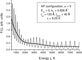
Figure 1: The typical dependence of the anomalous Green’s function $F(\omega,\xi,z)$ on the energy $\xi=\kappa^{2}/2m-\varepsilon_{F}$ under given $\Delta=9.25$ K, $\omega=0$, $z=0$ and $\varepsilon_{\rm ex}=0$, mean free paths in the F-layer are $l_{\uparrow}=120$ Å and $l_{\downarrow}=40$ Å, Fermi momentum $k_{F}=0.826$ Å^-1. $F(\xi)$ exhibits quantum oscillations, the smooth line shows function $F(\xi)$ averaged over oscillations, i.e. $F_{0}(\xi)$ (see the text for the details).

Using Eq. (13), we get expression for $F(\omega,\xi,z=z^{\prime})$:

$$F(\omega,\xi,z=z^{\prime})\ =\ 2m\sum_{\mu,\rho=\uparrow\downarrow}\varphi^{-}_{\mu}(z)\langle a_{\mu\rho}\rangle\psi^{+}_{\rho}(z)$$

where $\varphi^{-}_{\mu}(z)$ and $\psi^{+}_{\rho}(z)$ are the components of solutions $\varphi_{\mu}(z)$ and $\psi_{\rho}(z)$ in the S-layer. Denote

$$\theta_{1}\pm i\delta_{1}=k_{\pm}(d+z),\quad\theta_{2}\pm i\delta_{2}=k_{\pm}(d-z),$$

then $\theta_{1}+\theta_{2}=\theta$, $\delta_{1}+\delta_{2}=\delta$ and

$$\varphi_{\mu}^{-}(z) = \Lambda_{+}^{\mu}e^{i\theta_{1}}+\Lambda_{-}^{\mu}e^{-i\theta_{1}},$$

$$\psi_{\rho}^{+}(z) = \Sigma_{+}^{\rho}e^{i\theta_{2}}+\Sigma_{-}^{\rho}e^{-i\theta_{2}},$$

where

$$\Lambda_{+}^{\mu}=\alpha A_{+}^{\mu}e^{-\delta_{1}}+B_{+}^{\mu}e^{\delta_{1}}, \Lambda_{-}^{\mu}=\alpha A_{-}^{\mu}e^{\delta_{1}}+B_{-}^{\mu}e^{-\delta_{1}},$$

$$\Sigma_{+}^{\rho}=C_{-}^{\rho}e^{-\delta_{2}}+\alpha D_{-}^{\rho}e^{\delta_{2}}, \Sigma_{-}^{\rho}=C_{+}^{\rho}e^{\delta_{2}}+\alpha D_{+}^{\rho}e^{-\delta_{2}}.$$

The higher order terms with $e^{\pm in\theta}$, where $n\geq 2$, can be dropped in the expansion (16) because they are responsible for rapid oscillations of $F(\xi)$. Finally, we come to the following expression for the anomalous Green’s function in the S-layer,

$$F(\omega,\xi,z=z^{\prime})=F_{0}(\omega,\xi,z)+F_{1}(\omega,\xi,z),$$

where

$$F_{0}(\omega,\xi,z) = 2m\sum_{\mu\rho}\Bigl{\{}\Lambda_{+}^{\mu}\Sigma_{+}^{\rho}b_{\mu\rho}^{-}+\Lambda_{-}^{\mu}\Sigma_{-}^{\rho}b_{\mu\rho}^{+}\Bigr{\}},$$ (17)

$$F_{1}(\omega,\xi,z) = 2m\sum_{\mu\rho}\Bigr{\{}\Lambda_{+}^{\mu}\Sigma_{-}^{\rho}\Bigl{[}b_{\mu\rho}^{+}e^{2i\theta_{1}}+b_{\mu\rho}^{-}e^{-2i\theta_{2}}\Bigr{]}$$

$$+ \Lambda_{-}^{\mu}\Sigma_{+}^{\rho}\Bigl{[}b_{\mu\rho}^{+}e^{2i\theta_{2}}+b_{\mu\rho}^{-}e^{-2i\theta_{1}}\Bigr{]}\Bigr{\}}.$$

The contribution $F_{1}$ to the function $F$ is essential only in the vicinity of S/F interfaces, $z=\pm d$, as far as $\theta_{1}\sim(z+d)$ and $\theta_{2}\sim(d-z)$. At the point $z=z^{\prime}=0$ (the middle of the S-layer) the anomalous Green’s function is determined by the function $F_{0}(\omega,\xi,z)$ which is shown by the thick smooth line in Fig. 1. The obtained result is used below in Sec. IV where we discuss the self-consistent evaluation of the order parameter.

III.2 F-layer

Due to proximity effect, the correlations between electrons are induced in the ferromagnet close to the supercoducting layer. Instead of simple decay, as it would be for the superconductor/normal-metal interface, in the case of ferromagnetic layer the Cooper pair wave function exhibits the damping oscillatory behavior in the ferromagnet with increasing a distance from the S/F interface Buzdin_JETP ; Buzdin_PRB ; Demler . The reason is that exchange splitting of bands in the F-region changes the pairing conditions for electrons, therefore the Cooper pairs are formed from quasiparticles with equal energies but with different in modulus momenta $p_{\uparrow}$ and $-p_{\downarrow}$. Due to the non-zero center of mass momentum $\Delta p$, the Cooper pair wave function obtains the spatially dependent phase in the ferromagnetic layer. In the ”clean” limit (no scattering in the ferromagnet) one can find Demler that the Cooper pair wave function oscillates with the distance $z$ into the F-layer as $\sim\sin(z/\xi_{F}^{0})/(z/\xi_{F}^{0})$ where $\xi_{F}^{0}=v_{F}/\varepsilon_{\rm ex}$.

This result holds also in the case of ”dirty” ferromagnet. The microscopic theory of S/F multilayers based on the quasiclassical Usadel equations Buzdin_JETP ; Buzdin_PRB predicts that the anomalous Green’s function behaves in the ferromagnet as $\sim\exp\{-(1+i)\sqrt{h/D_{M}}z\}$, where $D_{M}=v_{F}l/3$ is the diffusion coefficient and $l$ is the electron mean free path in the F-layer. Therefore, a length scale for oscillations and damping is the same and this scale is set by the length $\xi_{M}=\sqrt{2l\xi_{F}^{0}/3}$. Below in this section it is shown that in the framework of our model the scales for oscillations and damping of the anomalous Green’s function are determined by different lengths.

We can find the anomalous Green’s function $F(\omega,\xi,z=z^{\prime})$ in the F-region $(d<z<a)$ following the same approach that was used to evaluate the $F$-function in the superconductor. The solutions $\psi_{\uparrow(\downarrow)}(z)$ in the layer F₃ $(d<z<a)$ are given by Eq. (8). For the solutions $\varphi_{\mu}(z)$ ($\mu=\uparrow,\downarrow$) we can write

$$\varphi_{\mu}(z) =\displaystyle X^{\mu}_{+}\left(1\atop 0\right)e^{ip_{3}^{\uparrow}(a-z)}+X^{\mu}_{-}\left(1\atop 0\right)e^{-ip_{3}^{\uparrow}(a-z)}$$

$$\displaystyle+\ Y^{\mu}_{+}\left(0\atop 1\right)e^{ip_{3}^{\downarrow}(a-z)}+Y^{\mu}_{-}\left(0\atop 1\right)e^{-ip_{3}^{\downarrow}(a-z)},$$

where $X^{\mu}_{\pm}$ and $Y^{\mu}_{\pm}$ can be found from conditions of continuity of the functions $\varphi_{\mu}(z)$ and their derivatives at $z=d$, assuming perfect S/F interface.

The anomalous Green’s function averaged over oscillations is

$$F(\omega,\xi,z=z^{\prime}) = 2m\sum_{\mu}\varphi_{\mu}^{-}(z)\langle a_{\mu\uparrow}\rangle\psi_{\uparrow}^{+}(z)$$ (18)

$$= 2m\sum_{\mu}F_{\mu}\langle a_{\mu\uparrow}\rangle.$$

It turns out that function $\varphi_{\mu}^{-}(z)$ contains four terms with multipliers $e^{\pm\theta_{+}}$ and $e^{\pm\theta_{-}}$. Denoting $\theta_{\pm}=\theta\pm i\delta$, we can write $F_{\mu}$ in the form

$$F_{\mu}=\Phi_{\mu}^{+}e^{i\theta}+\Phi_{\mu}^{-}e^{-i\theta},$$ (19)

where

$$\Phi_{\mu}^{+} = \Bigl{[}\Theta_{+}^{\mu}\cos(p_{3}^{\downarrow}z_{1})+\Xi_{+}^{\mu}\sin(p_{3}^{\downarrow}z_{1})\Bigr{]}$$ (20)

$$\times \sin[p_{3}^{\uparrow}(d_{F}-z_{1})],$$

$$\Phi_{\mu}^{-} = \Bigl{[}\Theta_{-}^{\mu}\cos(p_{3}^{\downarrow}z_{1})+\Xi_{-}^{\mu}\sin(p_{3}^{\downarrow}z_{1})\Bigr{]}$$

$$\times \sin[p_{3}^{\uparrow}(d_{F}-z_{1})],$$

here $z_{1}=z-d$ is the distance from the S/F interface, and

$$\Theta^{\mu}_{+} = B^{\mu}_{+}e^{\delta}+\alpha A^{\mu}_{+}e^{-\delta},$$

$$\Theta^{\mu}_{-} = \alpha A^{\mu}_{-}e^{\delta}+B^{\mu}_{-}e^{-\delta},$$

$$\Xi^{\mu}_{+} = \frac{ik_{-}}{p_{3}^{\downarrow}}B_{\mu}^{+}e^{\delta}+\alpha\frac{ik_{+}}{p_{3}^{\downarrow}}A^{\mu}_{+}e^{-\delta},$$

$$\Xi^{\mu}_{-} = -\left(\alpha\frac{ik_{+}}{p_{3}^{\downarrow}}A^{\mu}_{-}e^{\delta}+\frac{ik_{-}}{p_{3}^{\downarrow}}B^{\mu}_{-}e^{-\delta}\right).$$

Using Eqs. (16), (18), (19) we get the expression for function $F$ averaged over the rapid oscillations

$$F(\omega,\xi,z=z^{\prime})=2m\sum_{\mu}\left[\Phi_{\mu}^{-}b_{\mu\uparrow}^{+}+\Phi_{\mu}^{+}b_{\mu\uparrow}^{-}\right].$$

It follows from Eq. (20) for $\Phi_{\mu}^{\pm}$, that the dependence of function $F(\omega,\xi,z)$ on variable $z$ or $z_{1}=z-d$ is given by a sum of the terms with sine and cosine from arguments $(p_{3}^{\uparrow}+p_{3}^{\downarrow})z_{1}$ and $(p_{3}^{\uparrow}-p_{3}^{\downarrow})z_{1}$. The terms with phases $(p_{3}^{\uparrow}+p_{3}^{\downarrow})z_{1}$ determine the short-periodic oscillations with respect to oscillations with larger period $\sim(p_{3}^{\uparrow}-p_{3}^{\downarrow})^{-1}$. Neglecting the nonessential terms with short-periodic oscillations, the anomalous Green’s function can be presented in the form

$$F(\omega,\xi,z=z^{\prime}) = \widetilde{\Theta}(\omega,\xi)\cos(\Delta p_{3}z_{1})$$

$$+ \widetilde{\Xi}(\omega,\xi)\sin(\Delta p_{3}z_{1}),$$

where $z_{1}=z-d$, $\Delta p_{3}=p_{3}^{\uparrow}-p_{3}^{\downarrow}$, and $p_{3}^{\uparrow(\downarrow)}$ are given by Eqs. (9), (10).

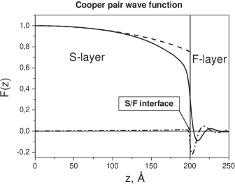
Figure 2: The behavior of the anomalous Green’s function $F(z)$ along the F/S/F structure with $d_{S}=400$ Å, $d_{F}=50$ Å, $\varepsilon_{\rm ex}=1.156$ eV, $l_{\uparrow}=133$ Å, $l_{\downarrow}=35$ Å. The point $z=200$ Å is the S/F interface. Solid line — Re $F(z)$, dashed dotted line — Im $F(z)$. The contribution Re $F_{0}(z)$ [see Eq. (17)] to the function Re $F(z)$ in the S-layer is shown by dashed line.

The real and imaginary parts of the function

$$F(z)=T\sum_{\omega}\int_{0}^{\varepsilon_{F}}d\xi\ F(\omega,\xi,z)$$

normalized on the value of its real part at the point $z=0$ (the middle of the S-layer) are shown in Fig. 2. The dashed line in Fig. 2 shows the contribution $F_{0}(z)$ [see Eq. (17)] to the function $F(z)$ in the S-layer. We can estimate the lengths responsible for the oscillations and decay using Eq. (10) for momenta $p_{3}^{\uparrow}$ and $p_{3}^{\downarrow}$. Neglecting $\pm i\omega$ in Eq. (10), since $|\omega|\leq\omega_{D}$, we obtain

$$p_{3}^{\uparrow(\downarrow)}=\sqrt{2m(\xi\pm h)}\left[1\pm\frac{i}{4}\tau^{-1}_{\downarrow(\uparrow)}\frac{1}{\xi\pm h}+\dots\ \right]$$

As far as the integration over $\xi$ goes from $0$ till $\varepsilon_{F}$, then the damping of oscillations is determined by the value

$$\sim\frac{1}{l_{0}}=\frac{1}{l_{\uparrow}}+\frac{1}{l_{\downarrow}}.$$

Neglecting $\pm i\tau^{-1}_{\downarrow(\uparrow)}$ and $\pm i\omega$ in Eq. (10), we get

$$p_{3}^{\uparrow(\downarrow)}=\sqrt{2m\xi}\left[1\pm\frac{h}{2\xi}+\dots\ \right].$$

If $\xi\sim\varepsilon_{F}$, then

$$\Delta p_{3}z_{1}\sim\frac{\varepsilon_{\rm ex}}{v_{F}}z_{1}=\frac{\pi z_{1}}{\xi_{m}^{0}},$$

where $\xi_{m}^{0}=\pi v_{F}/\varepsilon_{\rm ex}=\pi\xi_{F}^{0}$ is the half-period of oscillations of $F(z)$ (the distance between the nearest zeros). Note, that $\xi_{m}^{0}\neq\pi l_{0}$ in contrast to what is found by using a quasiclassical approach.

The oscillatory terms in Eq. (III.2) arise due to quantum interference between two plane waves describing an electron and a hole propagating in the ferromagnetic layer with different momenta $p_{3}^{\uparrow}$ and $-p_{3}^{\downarrow}$ along the $z$-axis. If $h\neq 0$ then $\Delta p_{3}\neq 0$, and the oscillatory dependence of the Cooper pair wave function occurs due to the exchange field in the ferromagnet. If $h=0$, then $F(z)$ exhibits only the exponential decay into the F-layer with characteristic length $l_{0}$. As it was already pointed out by many authors, the physical picture of the proximity effect is similar to the nonuniform Fulde-Ferrel-Larkin-Ovchinnikov (FFLO) state FF ; LO which is characterized by the oscillatory dependent order parameter and arises in a homogeneous superconductor in the presence of a strong enough uniform exchange field.

IV Self-consistent evaluation of the order parameter

In this section we proceed further by constructing the self-consistent solution of Eqs. (1,2,4). In case of antiparallel orientation of magnetizations in the ferromagnetic layers the self-consistency can be reached if the order parameter $\Delta(z)$ takes the real values. We will search the self-consistent solution of Eq. (4) in the S-layer assuming that in this equation the function $F(\omega,\xi,z)$ is replaced by its first contribution $F_{0}(\omega,\xi,z)$ given by Eq. (17). Function $F_{0}(z)$ is shown by dashed line in Fig. 2 and can be approximated by a simple analytical function on $z$ like $\propto\cos(qz)$, where $q$ is a parameter. In order to take into account the correction $F_{1}(z)$ one has to choose a more complex class of sample functions for $\Delta(z)$. However, this will not change the results significantly.

Let us look for $\Delta(z)$ in the form

$$\Delta(z)=\Delta\cos(qz)\simeq\Delta\left(1-\frac{q^{2}z^{2}}{2}\right),$$

where the wave vector $q$ (which has to be found) is small. The magnitude $\Delta(d)=(1-\delta_{0})\Delta$ defines the amplitude of the superconducting order parameter at the S/F interface (see Fig. 2), here $\delta_{0}=q^{2}d^{2}/2\sim 0.1$ is a small parameter. Following the well-known WKB-approximation WKB , we search the solutions of Schrödinger’s equation (6) in the form

$$\psi(z)=\left(e^{i\xi_{+}(z)}\atop e^{i\xi_{-}(z)}\right).$$

For $\xi_{\pm}$ we get the system of equations

$$\left[i\omega+\xi+\frac{1}{2m}\left(i\xi^{\prime\prime}_{+}-\xi_{+}^{\prime 2}\right)\right]e^{i\xi_{+}}+\Delta(z)e^{i\xi_{-}}=0,$$ (22)

$$\Delta^{*}(z)e^{i\xi_{+}}+\left[i\omega-\xi-\frac{1}{2m}\left(i\xi^{\prime\prime}_{-}-\xi_{-}^{\prime 2}\right)\right]e^{i\xi_{-}}=0,$$

where $\xi=\varepsilon_{F}-\kappa^{2}/2m$ and primes above $\xi_{\pm}$ denote the derivatives by $z$.

In case of $q=0$, $\Delta(z)=\Delta$, four solutions of system (22) are $\xi_{+}^{0}=\pm k_{+}z$, $\xi_{-}^{0}=\pm k_{+}z+i\log\alpha$ and $\xi_{+}^{0}=\pm k_{-}z+i\log\alpha$, $\xi_{-}^{0}=\pm k_{-}z$ which give four initial eigenfunctions of the non-perturbed Eq. (6) ($q=0$):

$$u_{\pm}^{0}(z)=\left(1\atop\alpha\right)e^{\pm ik_{+}z},\quad v_{\pm}^{0}(z)=\left(\alpha\atop 1\right)e^{\pm ik_{-}z}.$$

Consider, for example, the perturbed solution $u_{+}(z)$ which corresponds to $u_{+}^{0}(z)$ in the case of $q\neq 0$. We look for the phases $\xi_{\pm}$ in the form $\xi_{\pm}=\xi_{\pm}^{0}+\eta_{\pm}$, where $\xi_{+}^{0}=k_{+}z$, $\xi_{-}^{0}=k_{+}z+i\log\alpha$ for $u_{+}^{0}(z)$. The typical order of $\eta_{\pm}$ is $\sim qz\sim qd=\sqrt{2\delta_{0}}<1$. By linearizing the system (22) with respect to $\eta_{\pm}$ we come to the following equations

$$-\frac{1}{\alpha}\frac{k_{+}}{m}\ \eta_{+}^{\prime}+i\Delta(\eta_{-}-\eta_{+})=\Delta\frac{q^{2}z^{2}}{2},$$ (23)

$$\alpha\frac{k_{+}}{m}\ \eta_{-}^{\prime}-i\Delta(\eta_{-}-\eta_{+})=\Delta\frac{q^{2}z^{2}}{2}.$$

We also have dropped the terms with $\eta_{\pm}^{\prime 2}$ and $\eta_{\pm}^{\prime\prime}$ which are small as compared to $k_{\pm}\eta_{\pm}^{\prime}$, since $\eta_{\pm}^{\prime 2}\sim\eta_{\pm}^{\prime}\eta_{\pm}/d\sim\eta_{\pm}^{\prime}\sqrt{2\delta_{0}}/d\ll k_{\pm}\eta_{\pm}^{\prime}$ if $d\sim 200$ Å and $k_{\pm}\sim 0.5$ Å^-1, and $\eta_{\pm}^{\prime\prime}\sim\eta_{\pm}^{\prime}/d\ll k_{\pm}\eta_{\pm}^{\prime}$. The equations similar to Eqs. (23) can be written also for phases $\eta_{\pm}$ which determine other three solutions $u_{-}(z)$ and $v_{\pm}(z)$. Solving these equations we get

$$u_{\pm}(z)=\left({\ e^{\pm i[k_{+}z+\eta_{+}^{(\pm)}(z)]}}\atop{\alpha e^{\pm i[k_{+}z+\eta_{-}^{(\pm)}(z)]}}\right),$$

with

$$\eta_{\pm}^{(+)}(z) = \tau_{3}^{\pm}z^{3}+\tau_{2}^{\pm}z^{2}+\tau_{1}^{\pm}z+\tau_{0}^{\pm},$$

$$\eta_{\pm}^{(-)}(z) = \tau_{3}^{\pm}z^{3}-\tau_{2}^{\pm}z^{2}+\tau_{1}^{\pm}z-\tau_{0}^{\pm};$$

and

$$v_{\pm}(z)=\left({\alpha e^{\pm i[k_{-}z+\zeta_{+}^{(\pm)}(z)]}}\atop{\ e^{\pm i[k_{-}z+\zeta_{-}^{(\pm)}(z)]}}\right),$$

where

$$\zeta_{\pm}^{(+)}(z) = \rho_{3}^{\pm}z^{3}+\rho_{2}^{\pm}z^{2}+\rho_{1}^{\pm}z+\rho_{0}^{\pm},$$

$$\zeta_{\pm}^{(-)}(z) = \rho_{3}^{\pm}z^{3}-\rho_{2}^{\pm}z^{2}+\rho_{1}^{\pm}z-\rho_{0}^{\pm}.$$

The expressions for coefficients $\tau^{\pm}_{i}$ and $\rho^{\pm}_{i}$ of polynomials are given in Appendix B.

Next the procedure of evaluation of the anomalous Green’s function in the S-layer is similar to one described in details in Secs. II and III for the case of $\Delta(z)=\Delta$. By representing the solutions $\varphi_{\mu}(z)$ and $\psi_{\mu}(z)$ of Eq. (6) as a linear combination of eigenfunctions $u_{\pm}(z)$ and $v_{\pm}(z)$ similar to representation (11), we can find the new coefficients $A^{\mu}_{\pm}$, $B^{\mu}_{\pm}$, $C^{\mu}_{\pm}$, $D^{\mu}_{\pm}$ solving the system of 4 linear equations. By evaluating the currents $j_{\mu\rho}$ at the point $z=0$ ($j_{\mu\rho}$ do not depend on $z$), we obtain the expressions for $j_{\mu\rho}$ similar to Eq. (III.1) where $k_{\pm}$ should be replaced by

$$\widetilde{k}_{+}=k_{+}+\frac{\tau_{1}^{+}-\alpha^{2}\tau_{1}^{-}}{1-\alpha^{2}},\quad\widetilde{k}_{-}=k_{-}+\frac{\rho_{1}^{-}-\alpha^{2}\rho_{1}^{+}}{1-\alpha^{2}},$$

and $\theta_{\pm}=2ik_{\pm}d=\theta\pm i\delta$. The substitutions $k_{\pm}\to\widetilde{k}_{\pm}$ also have to be made in Eq. (III.1) for $a_{\mu\rho}$ and in the expression for $\mathrm{det}J$ (see Appendix A). Finally, the anomalous Green’s function $F(\omega,\xi,z)$ is given by Eqs. (17) where $\Lambda_{\pm}^{\mu}$ and $\Sigma_{\pm}^{\rho}$ are replaced by new functions $\widetilde{\Lambda}_{\pm}^{\mu}$ and $\widetilde{\Sigma}_{\pm}^{\rho}$:

$$\widetilde{\Lambda}^{\mu}_{+} = \alpha A^{\mu}_{+}e^{-\delta_{1}+i\eta_{-}^{(+)}}+B^{\mu}_{+}e^{\delta_{1}+i\zeta_{-}^{(+)}},$$

$$\widetilde{\Lambda}^{\mu}_{-} = \alpha A^{\mu}_{-}e^{\delta_{1}-i\eta_{-}^{(-)}}+B^{\mu}_{-}e^{-\delta_{1}-i\zeta_{-}^{(-)}},$$

$$\widetilde{\Sigma}^{\rho}_{+} = C^{\rho}_{-}e^{-\delta_{2}-i\eta_{+}^{(-)}}+\alpha D^{\rho}_{-}e^{\delta_{2}-i\zeta_{+}^{(-)}},$$

$$\widetilde{\Sigma}^{\rho}_{-} = C^{\rho}_{+}e^{\delta_{2}+i\eta_{+}^{(+)}}+\alpha D^{\rho}_{+}e^{-\delta_{2}+i\zeta_{+}^{(+)}},$$

here $\delta_{1}$, $\delta_{2}$, $\eta_{\pm}^{(\pm)}$ and $\zeta_{\pm}^{(\pm)}$ are functions on $z$. The fixed point $q=q_{*}$ which determines the order parameter $\Delta(z)$ has to be found numerically by solving Eq. (4) using the iterative procedure.

V Critical temperature $T_{c}$

If the anomalous Green’s function in the S-region $F(\omega,\xi,z)=F(\omega,\xi,z=0)\cos(q_{*}z)$ is known, the superconducting transition temperature $T_{c}$ can be found. Up to now we assume the ”clean” limit for a superconductor. The corrections (3) due to scattering will be taking into account further. Let us introduce the function

$$F_{\omega}=\frac{1}{k_{F}}\int_{0}^{\varepsilon_{F}}d\xi\ F(\omega,\xi,z=0),$$

where $k_{F}$ is Fermi momentum in the S-layer. This integral can be evaluated only numerically. However, we can approximate $F_{\omega}$ by the analytical function of argument $\omega$. Let us represent $F_{\omega}$ in the form

$$F_{\omega}=\frac{\Delta}{\sqrt{\omega^{2}+\Delta^{2}}}\ F^{(1)}_{\omega}.$$

For the bulk superconductor $F^{(1)}_{\omega}=1$. Let $T\to T_{c}$, therefore $\Delta\ll\Delta(0)$, where $\Delta(0)$ is the order parameter at $T=0$. If $\omega$ takes values from $0$ till $\sim 5\omega_{D}$, $F^{(1)}_{\omega}$ can be well approximated by the following function

$$F^{(1)}_{\omega}\simeq A_{0}\tanh\left(\frac{\gamma_{0}|\omega|}{2\omega_{D}}\right).$$ (24)

The coefficients $A_{0}$ and $\gamma_{0}$ are found numerically by minimizing the norm of a difference between the exact and approximate function. These coefficients are non-monotonic functions of the F-layer thickness $d_{F}$ when $d_{S}$ is fixed. For typical values of the parameters describing the F/S/F structure the magnitudes of $A_{0}$ and $\gamma_{0}$ are $A_{0}\sim 0.9$ and $\gamma_{0}\sim 4.0$.

The scattering in the S-layer is introduced by Eq. (3). Numerical analysis shows that in Eq. (3) the Green’s function $G_{\uparrow\uparrow}^{ss}(z,z)$ does not depend on $z$ in the S-region and its real part is negligibly small. Obviously, $\Delta_{\omega}(z)=\Delta_{\omega}\cos(q_{*}z)$. From numerical analysis it follows that $G_{\omega}$ in the S-layer can be represented as

$$G_{\omega} = \frac{1}{k_{F}}\int_{0}^{\varepsilon_{F}}d\xi\ G_{\uparrow\uparrow}^{ss}(\omega,\xi,z=0)$$ (25)

$$\approx -A_{0}\frac{i\omega}{\sqrt{\omega^{2}+\Delta^{2}}}.$$

Taking into account Eqs. (24) and (25), equations (3) can be written in the form similar to the case of bulk superconductor Svidz :

$$\omega^{\prime} \approx \omega+\frac{A_{0}}{2\tau_{0}}\ \frac{\omega^{\prime}}{\sqrt{\omega^{{}^{\prime}2}+\Delta_{\omega}^{2}}},$$

$$\Delta_{\omega} \approx \Delta+\frac{A_{0}}{2\tau_{0}}\ \frac{\Delta_{\omega}}{\sqrt{\omega^{{}^{\prime}2}+\Delta_{\omega}^{2}}},$$ (26)

where $\tau_{0}^{-1}=2\pi cu_{0}^{2}N(\varepsilon_{F})$ is the inverse life-time of quasiparticles in the superconductor, and $N(\varepsilon_{F})=mk_{F}/2\pi^{2}$ is density of states at the Fermi energy. Deriving Eq. (26) we took into account that, if $\frac{1}{2}\tau_{0}^{-1}\sim\omega_{D}\sim 300$ K corresponding to mean free path $l_{s}\sim 130$ Å, then for $\omega^{\prime}\simeq\omega+{A_{0}}/{2\tau_{0}}$ and $\gamma_{0}\sim 4.0$ we have $\tanh\left(\gamma_{0}|\omega^{\prime}|/2\omega_{D}\right)\approx 1$.

Equations (26) can be written as Svidz

$$\omega^{\prime}=\omega\eta(\omega),\quad\Delta_{\omega}=\Delta\eta(\omega),$$

$$\eta(\omega)=1+\frac{A_{0}}{2\tau_{0}\sqrt{\omega^{2}+\Delta^{2}}}.$$ (27)

Using (27) and (4) we come to the equation for $T_{c}$:

$$\pi\rho T_{c}\sum_{\omega}\frac{1}{|\omega|}\tanh\left(\frac{\gamma_{0}|\omega^{\prime}|}{2\omega_{D}}\right)=1,$$ (28)

where

$$\omega^{\prime}=\omega+\frac{A_{0}}{2\tau_{0}},\quad\rho=\rho_{0}A_{0}<\rho_{0},$$

and $\rho_{0}=\lambda N(\varepsilon_{F})$ is the renormalized coupling constant. By carrying out the summation over Matsubara frequencies $\omega=\pi T_{c}(2n+1)$ in Eq. (28), we get the equation for reduced critical temperature $\tau=T_{c}/T_{c}^{0}$:

$$\tau=\exp\left\{\left(\frac{1}{\rho_{0}}-\frac{1}{\rho}\right)-\Phi\Bigl{[}\eta_{0}(\tau)\Bigr{]}\right\},$$ (29)

where

$$\Phi(\eta_{0})=\sum_{n=0}^{+\infty}\frac{4\Gamma_{0}e^{-(2n+1)\eta_{0}}}{(2n+1)(1+\Gamma_{0}e^{-(2n+1)\eta_{0}})},$$

$$\eta_{0}(\tau)=\frac{\gamma_{0}\pi T_{0}}{\omega_{D}}\tau,\quad\tau=T_{c}/T_{c}^{0},$$

$$\Gamma_{0}=\exp\left(-\frac{\gamma_{0}A_{0}}{2\tau_{0}\omega_{D}}\right),$$

and $T_{c}^{0}=2\pi^{-1}\omega_{D}\gamma e^{-1/\rho_{0}}$ ($\gamma=e^{C},\ C=0.577\dots\$) is transition temperature of the bulk superconductor.

VI Results and discussion

In this section we present the results of numerical calculation of the critical temperature $T_{c}$. We first focus on the general features of a behavior of the system. Next we consider selected experimental data which can be interpreted in the framework of the given model.

VI.1 Oscillatory behavior of $T_{c}$

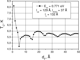
Figure 3: Critical temperature $T_{c}$ for the F/S/F trilayer as a function of the ferromagnetic layer thickness $d_{F}$. The parameters are $\varepsilon_{\rm ex}=0.771$ eV (exchange field in the ferromagnet), $l_{\uparrow}=129$ Å, $l_{\downarrow}=37$ Å, $l_{s}=132$ Å(mean free paths in the F and S layers), $k_{F}=0.826$ Å^-1 (Fermi momentum in the superconductor), $\omega_{D}=275$ K, $T_{c}^{0}=9.25$ K.

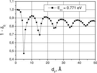
Figure 4: The dependence of the normalized amplitude $(1-\delta_{0})$ of the superconducting order parameter at the S/F interface as a function of the F-layer thickness $d_{F}$ for the same parameters as in Fig. 3.

The typical dependence of critical temperature $T_{c}(d_{F})$ with respect to ferromagnetic layer thickness $d_{F}$ with $d_{S}=400$ Å is shown in Fig. 3 where the model parameters are given in the figure caption. The effective electron mass is $m=m_{e}$ ($m_{e}$ is a bare electron mass). For superconductor we took $\omega_{D}=276$ K and $T_{c}^{0}=9.25$ K which are the parameters of bulk Nb. The corresponding normalized magnitude $(1-\delta_{0})$ of the order parameter at the S/F interface as a functions of $d_{F}$ is shown in Fig. 4.

Both functions $(1-\delta_{0})$ and $T_{c}(d_{F})$ show the pronounced damping oscillatory behavior with the same period. The oscillatory behavior of $T_{c}(d_{F})$ is a consequence of oscillations of the amplitude $\Delta(d)=\Delta(1-\delta_{0})$ of the order parameter at the S/F interface when $d_{F}$ is varying. The minima of $\Delta(d)$ correspond to minima of $T_{c}$ and the maxima of $\Delta(d)$ correspond to the maxima of $T_{c}$, as they should. The oscillations of $\Delta(d)$ in turn are caused by the oscillations of the anomalous Green’s function $F(z)$ in the F-layer. Function $F(z)$ must satisfy the zero boundary condition at the ferromagnet/vacuum interface. Because of oscillations of $F(z)$ in the F-region, the order parameter at the S/F interface is forced to adjust in such a way that the condition $F(a)=0$ is fulfilled at the outer boundary $z=a$ of the F-layer.

Table 1: The comparison of the periods of oscillations $\xi_{F}$ predicted by formula (30) with the period $\widetilde{\xi}_{F}$ obtained from numerical analysis for different values of exchange field $\varepsilon_{\rm ex}$, effective electron mass $m$ and a superconductor layer thickness $d_{S}$. Other model parameters are the same as in Fig. 3. The accuracy of determining of $\widetilde{\xi}_{F}$ is restricted by a finite step for $d_{F}$ in numerical calculations.

$\varepsilon_{\rm ex}$ (eV)	$m\ (m_{e})$	$d_{S}$ (Å)	$\xi_{F}$ (Å)	$\widetilde{\xi}_{F}$ (Å)
0.385	1.0	400	13.97	14.0
0.771	1.0	400	9.98	10.0
1.156	1.0	400	8.06	8.0
2.027	1.0	400	6.09	6.0
0.610	0.45	600	16.55	16.5

The results of numerical analysis, presented in Table I for different values of exchange field $\varepsilon_{\rm ex}$ and effective electron mass $m$, show that the period $\xi_{F}$ of $T_{c}$-oscillations is defined as

$$\xi_{F}=\frac{\pi}{\sqrt{m\varepsilon_{\rm ex}}}=\sqrt{\pi\xi_{m}^{0}k_{F}^{-1}},$$ (30)

here $k_{F}$ is the Fermi momentum in a superconductor. The period $\xi_{F}$, therefore, does not depend on the electron mean free paths in the S- and F-layers. The first minimum of $T_{c}(d_{F})$ occurs at the thickness $\xi_{F}/2$, while the location of first maximum is $\xi_{F}$.

As can be seen from Fig. 5, the strong scattering in the ferromagnetic layers significantly damps the oscillations of $T_{c}$, but their period remains unchanged for any values of the mean free paths $l_{\uparrow}$ and $l_{\downarrow}$. As it follows from the analysis presented in Sec. III, the reason of such a behavior is that the strong scattering in the F-region affects only the length $l_{0}$ of decay of the Cooper pair wave function $F(z)$ but not the period $\sim\xi_{m}^{0}$ of its oscillations. The less pronounced are the oscillations of $F(z)$ with respect to $z_{1}=z-d$ in case of strong electron scattering, the less is the amplitude of oscillations of $\Delta(d)$ and $T_{c}$ with respect to the ferromagnetic layer thickness $d_{F}$. In case of extremely strong scattering, the coherent coupling which was established due to these oscillations between two boundaries of ferromagnetic layer is destroyed and thus the oscillations of $T_{c}$ are suppressed completely.

We also observed that strong scattering in the S layer (small mean free path $l_{s}$) suppresses the amplitude of $T_{c}$ oscillations (look at Fig. 6). The critical temperature is higher for smaller values of $l_{s}$ . The reason for it is that in the thin superconducting films $T_{c}$ is reduced with respect to $T_{c}^{0}$ due to dimensional effect, and the magnitude of $T_{c}$ depends on $d_{S}$ only via the dimensionless thickness $d_{S}/\xi_{S}$, where $\xi_{S}\propto\sqrt{\xi_{0}l_{s}}$ is a coherence length for the dirty superconductor, $\xi_{0}$ is a BCS coherence length. Small mean free path $l_{s}$, therefore, corresponds to large value of the effective film thickness $d_{S}/\xi_{S}$.

VI.2 Comparison with experiment

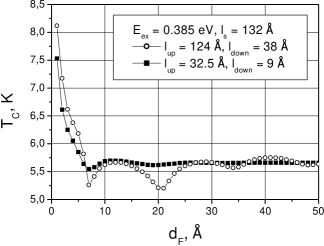
Figure 5: The critical temperature $T_{c}(d_{F})$ for the case of weak and strong scattering in the ferromagnetic layers; $\varepsilon_{\rm ex}=0.385$ eV, $l_{s}=132$ Å. Dots (weak scattering): $l_{\uparrow}=124$ Å, $l_{\downarrow}=38$ Å; squares (strong scattering): $l_{\uparrow}=32.5$ Å, $l_{\downarrow}=9$ Å.

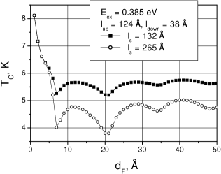
Figure 6: The critical temperature $T_{c}(d_{F})$ for different values of the mean free paths in the S-layer; $\varepsilon_{\rm ex}=0.385$ eV, $l_{\uparrow}=124$ Å, $l_{\downarrow}=38$ Å. Squares: $l_{s}=132$ Å; dots: $l_{s}=265$ Å.

Experimental situation on the oscillatory behavior of $T_{c}(d_{F})$ in the S/F structures is known to be controversial. Nevertheless, there are two groups of experiments described in the literature where oscillations of $T_{c}(d_{F})$ were clearly observed and the 3$d$ ferromagnets were used as F layers — these are reports on Fe/Nb/Fe trilayers by Mühge et al.Muhge , and Nb/Co and V/Co multilayers by Obi et al.Obi .

In Fig. 7 the fitting is shown to experimental data by Mühge et al. Muhge for Fe($d_{F}$)/Nb(400 Å)/Fe($d_{F}$) trilayers prepared by rf sputtering. According to formula (30) the period $\xi_{F}$ of oscillations is determined by exchange splitting energy in the ferromagnet. If we take the value $\varepsilon_{\rm ex}^{d}\simeq 0.149~{}{\rm Ry}=2.03$ eV (Ref. Moruzzi, ) of exchange splitting of the Fe $d$-bands near the Fermi energy and put $m=m_{e}$, we obtain $\xi_{F}^{(d)}=6.09$ Å (see Table I) which is too small as compared to the location of a maximum at $d_{F}\sim 10\div 15$ Å in Fig. 7. However, we can assume that in the S and F layers the Cooper pairs are formed by $s$ electrons of Nb and Fe. The value of exchange splitting $\varepsilon_{\rm ex}^{s}=0.028~{}{\rm Ry}=0.381$ eV at the bottom of Fe $s$ bands ($\Gamma$ point, Ref. Moruzzi, ) together with $m=m_{e}$ gives the period $\xi_{F}=14.05$ Å. Thus, the first minimum of $T_{c}(d_{F})$ is at the point $\xi_{F}/2\approx 7$ Å, and the first maximum is at $\xi_{F}\approx 14$ Å. From Fig. 7 it follows that these values correlate with positions of minimum and maximum of $T_{c}$ which can be roughly determined from the scattered experimental points. We have put $\varepsilon_{F}=0.387$ Ry corresponding to the $s$ band of Nb (Ref. Moruzzi, ) which gives the Fermi momentum value $k_{F}=1.18$ Å^-1 for $m=m_{e}$. We used $\omega_{D}=276$ K and $T_{c}^{0}=9.25$ K for Nb. The fitting parameters are the values of mean free paths in Fe and Nb which were estimated approximately as $l_{\uparrow}=120$ Å, $l_{\downarrow}=40$ Å, and $l_{s}=269$ Å. Note, that magnetic measurements by Mühge et al. showed that thin Fe layers were not magnetic for $d_{F}\leq 7$ Å, and it was assumed that magnetically ”dead” Fe-Nb alloy of a thickness about 7 Å was formed at the interfacial S/F region for all samples with different $d_{F}$. Mühge et al. qualitatively explained the observed non-monotonic behavior of $T_{c}(d_{F})$ in terms of a rather complex behavior of this magnetically ”dead” Fe-Nb layer when $d_{F}$ was varying (see details in Ref. Muhge, ). They also argued that a non-monotonic $T_{c}(d_{F})$ behavior in their case could not be possible due to the mechanism of $\pi$ coupling as it was predicted for the S/F multilayers because of a single S layer in the trilayer system. Indeed, the well-known theoretical prediction by Buzdin et al. Buzdin_JETP ; Buzdin_PRB ascribes the oscillatory behavior of $T_{c}(d_{F})$ to the periodical switching of the ground state energy between 0- and $\pi$-phases of the order parameter if the neighboring S-layers in the S/F multilayer are coupled. However, it follows from the above analysis that the oscillatory behavior of $T_{c}(d_{F})$ does not necessary require the $\pi$ coupling and can occur also for a trilayer (or bilayer) F/S/F structure.

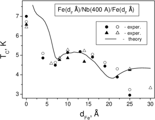
Figure 7: The comparison of the theoretical $T_{c}(d_{F})$ curve with experiment by Mühge et al. (Ref. Muhge, ) for Fe/Nb(400Å)/Fe trilayers. The fitting parameters are $l_{\uparrow}=120$ Å, $l_{\downarrow}=40$ Å, $l_{s}=269$ Å.

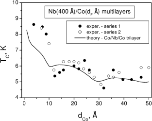
Figure 8: The comparison of the theoretical $T_{c}(d_{F})$ curve with experiment by Obi et al. (Ref. Obi, ) for Nb(400Å)/Co multilayers. The fitting parameters are $l_{\uparrow}=240$ Å, $l_{\downarrow}=80$ Å, $l_{s}=188$ Å.

Let us consider the experiments on Nb/Co multilayers by Obi et al. Obi . The theoretical curve $T_{c}(d_{F})$ in comparsion with experimental data is shown in Fig. 8. The exchange splitting of Co spin-up and down $s$ bands at $\Gamma$ point is $\varepsilon_{\rm ex}=0.014$ Ry (Ref. Moruzzi, ) which gives $\xi_{F}=19.87$ Å ($m=m_{e}$). The first and second minimum of $T_{c}(d_{F})$ should, therefore, be placed at points $d^{1}_{\rm min}=10$ Å and $d^{2}_{\rm min}=30$ Å. These values correlate with values 12 Å and 32 Å obtained from experiment. The fitting mean free paths are $l_{\uparrow}=240$ Å, $l_{\downarrow}=80$ Å, and $l_{s}=188$ Å. We have to note that in experiment Nb/Co structures are multilayers. A qualitative resemblance of theoretical $T_{c}$ curve calculated for a trilayer structure with experimental points for a multilayer and the agreement between theoretical and experimental values of $d^{1}_{\rm min}$ and $d^{2}_{\rm min}$ allows us to assume that neighboring S layers were decoupled in the experiment. As it was observed by Strunk et al. Strunk for similar Nb/Fe multilayered system (where F-layer is 3$d$ transition metal), the decoupling regime is set when $d_{F}$ is larger than some critical value $d_{c}^{\rm dc}$ which in turn is less than the critical thickness $d_{c}^{F}$ of the onset of ferromagnetism. This threshold value was $d_{c}^{F}\approx 7$ Å in experiments by Obi et al. Obi In Ref. Obi, it was noted that $d_{c}^{F}$ was less than the first minimum of $T_{c}$ at $d^{1}_{\rm min}\approx 12$ Å, so that for Nb/Co system the first minimum could not be ascribed to the onset of ferromagnetism as it was argued by Mühge et al. for the Fe/Nb/Fe systemMuhge . Our theoretical explanation assuming the decoupling regime is incorrect only for very thin Fe layers with $d_{F}<d_{c}^{\rm dc}$ when, probably, the Fe films are nonmagnetic due to alloying effect.

Note also, that experiments by Obi at el. Obi on Nb_1-xTi_x/Co multilayers with Nb_1-xTi_x alloy being superconductor with small coherence length did not reveal the oscillatory behavior of $T_{c}$ but showed only a small reduction of the critical temperature $T_{c}\approx 8$ K for large $d_{F}$ as compared to the bulk value $T_{c}^{0}\approx 9.2$ K (see Fig. 3 in Ref. Obi, ). Therefore, the observation of increasing of $T_{c}$ when the scattering is strong in S-layer together with damping of oscillations for small $l_{s}$ (see Fig. 6) is in a qualitative agreement with these experimental observations.

VII Summary

In conclusion, we have presented a theory of proximity effect in F/S/F trilayer nanostructures where S is a superconductor and F are layers of 3$d$ transition ferromagnetic metal. As a starting point of our calculations, we took the system of Gor’kov equations, which determine the normal and anomalous Green’s functions. The solution of these equations was found together with a self-consistent evaluation of the superconductor order parameter. In accordance with the known quasiclassical theories of proximity effect for S/F multilayers Buzdin_JETP ; Buzdin_PRB ; Demler ; Khusainov , we found that due to a presence of exchange field in the ferromagnet the anomalous Green’s function $F(z)$ exhibits damping oscillations in the F-layer as a function of a distance $z$ from the S/F interface. In the presented model a half-period of oscillations of $F(z)$ is determined by the length $\xi_{m}^{0}=\pi v_{F}/\varepsilon_{\rm ex}$, where $v_{F}$ is the Fermi velocity, $\varepsilon_{\rm ex}$ is the exchange field, and the length of damping is given by $l_{0}=(1/l_{\uparrow}+1/l_{\downarrow})^{-1}$, where $l_{\uparrow}$ and $l_{\downarrow}$ are spin-dependent mean free paths in the ferromagnetic layer. The oscillations of the anomalous Green’s function (Cooper pair wave function) in the F-region and a zero boundary condition at the ferromagnet/vacuum interface give rise to the oscillatory dependence of the superconductor order parameter at the S/F interface vs the F-layer thickness $d_{F}$. These oscillations result in oscillations of the superconductor transition temperature $T_{c}(d_{F})$ with a period $\xi_{F}=\pi/\sqrt{m\varepsilon_{\rm ex}}$. Thus we have demonstrated that the nonmonotonic oscillatory dependence of critical temperature $T_{c}(d_{F})$ does not necessarily require the mechanism of $\pi$-coupling between neighboring superconducting layers as it takes place in the S/F multilayers Buzdin_JETP ; Buzdin_PRB . The strong electron scattering either in the superconductor or in the ferromagnet significantly suppresses the oscillations. In case of extremely strong scattering in the ferromagnet the length of damping $l_{0}$ becomes very short and the oscillations of $T_{c}$ are suppressed completely. The reason of that is the loss of coherent ”coupling” between two boundaries of ferromagnetic layer that was established due to oscillations of Cooper pair wave function $F(z)$. We compared our results with existing data on $T_{c}(d_{F})$ for Fe/Nb/Fe trilayers Muhge and V/Co multilayers Obi , where F’s are 3$d$ ferromagnets, and found reasonable agreement with theory and experiment.

Appendix A

The determinant $\mathrm{Den}=\mathrm{det}J/(1-\alpha^{2})^{2}$ of the matrix of currents (Eq. 12) is given by the expression

$$\mathrm{Den}=-D_{0}+\Gamma_{+}e^{2i\theta}+\Gamma_{-}e^{-2i\theta},$$

where

$$D_{0} = 4k_{+}^{2}\left|\begin{array}[]{cc}A^{\uparrow}_{+}&A^{\downarrow}_{+}\\ A^{\uparrow}_{-}&A^{\downarrow}_{-}\end{array}\right|\times\left|\begin{array}[]{cc}C^{\uparrow}_{+}&C^{\downarrow}_{+}\\ C^{\uparrow}_{-}&C^{\downarrow}_{-}\end{array}\right|$$ (35)

$$+ 4k_{-}^{2}\left|\begin{array}[]{cc}B^{\uparrow}_{+}&B^{\downarrow}_{+}\\ B^{\uparrow}_{-}&B^{\downarrow}_{-}\end{array}\right|\times\left|\begin{array}[]{cc}D^{\uparrow}_{+}&D^{\downarrow}_{+}\\ D^{\uparrow}_{-}&D^{\downarrow}_{-}\end{array}\right|$$ (40)

$$+ 4k_{+}k_{-}e^{2\delta}\left|\begin{array}[]{cc}A^{\uparrow}_{-}&A^{\downarrow}_{-}\\ B^{\uparrow}_{+}&B^{\downarrow}_{+}\end{array}\right|\times\left|\begin{array}[]{cc}C^{\uparrow}_{+}&C^{\downarrow}_{+}\\ D^{\uparrow}_{-}&D^{\downarrow}_{-}\end{array}\right|$$ (45)

$$+ 4k_{+}k_{-}e^{-2\delta}\left|\begin{array}[]{cc}A^{\uparrow}_{+}&A^{\downarrow}_{+}\\ B^{\uparrow}_{-}&B^{\downarrow}_{-}\end{array}\right|\times\left|\begin{array}[]{cc}C^{\uparrow}_{-}&C^{\downarrow}_{-}\\ D^{\uparrow}_{+}&D^{\downarrow}_{+}\end{array}\right|,$$ (50)

$$\vskip 6.0pt plus 2.0pt minus 2.0pt\Gamma_{+} = 4k_{+}k_{-}\left|\begin{array}[]{cc}A^{\uparrow}_{+}&A^{\downarrow}_{+}\\ B^{\uparrow}_{+}&B^{\downarrow}_{+}\end{array}\right|\times\left|\begin{array}[]{cc}C^{\uparrow}_{-}&C^{\downarrow}_{-}\\ D^{\uparrow}_{-}&D^{\downarrow}_{-}\end{array}\right|,\vskip 6.0pt plus 2.0pt minus 2.0pt$$ (55)

$$\Gamma_{-} = 4k_{+}k_{-}\left|\begin{array}[]{cc}A^{\uparrow}_{-}&A^{\downarrow}_{-}\\ B^{\uparrow}_{-}&B^{\downarrow}_{-}\end{array}\right|\times\left|\begin{array}[]{cc}C^{\uparrow}_{+}&C^{\downarrow}_{+}\\ D^{\uparrow}_{+}&D^{\downarrow}_{+}\end{array}\right|,$$ (60)

and $A^{\mu}_{\pm}$, $B^{\mu}_{\pm}$, $C^{\mu}_{\pm}$, $D^{\mu}_{\pm}$ are coefficients introduced in Eq. (11).

Appendix B

Let us define the quantities

$$\lambda^{-1}_{\pm} = \frac{2m}{k_{\pm}}\sqrt{\omega^{2}+\Delta^{2}},$$

$$W_{\pm} = \frac{\Delta^{2}}{3}\left(\frac{m}{k_{\pm}}\right)^{2}q^{2},$$

$$V_{\pm} = \frac{q^{2}}{2}\left(\frac{m}{k_{\pm}}\right)\biggl{[}\frac{\omega^{2}}{\sqrt{\omega^{2}+\Delta^{2}}}\mp\omega\biggr{]}.$$

In case of $q\neq 0$ four linear independent solutions of Eq. (6) have the form:

i) solution $u_{+}(z)$:

$$u_{+}(z)=\left({\ e^{ik_{+}z+i\eta_{+}^{(+)}(z)}}\atop{\alpha e^{ik_{+}z+i\eta_{-}^{(+)}(z)}}\right),$$

where

$$\eta_{+}^{(+)}(z) = -\ i\lambda_{+}W_{+}z^{3}+i\lambda_{+}V_{+}z^{2}$$

$$+\ 2i\lambda_{+}^{2}V_{+}z+2i\lambda_{+}^{3}V_{+}$$

$$\equiv \tau_{3}^{+}z^{3}+\tau_{2}^{+}z^{2}+\tau_{1}^{+}z+\tau_{0}^{+},$$

$$\eta_{-}^{(+)}(z) = \frac{1}{\alpha^{2}}\ \eta_{+}^{(+)}(z)+\frac{\Delta}{3\alpha}\left(\frac{m}{k_{+}}\right)q^{2}z^{3}$$

$$\equiv \tau_{3}^{-}z^{3}+\tau_{2}^{-}z^{2}+\tau_{1}^{-}z+\tau_{0}^{-};$$

ii) solution $u_{-}(z)$:

$$u_{-}(z)=\left({\ e^{-ik_{+}z-i\eta_{+}^{(-)}(z)}}\atop\alpha{e^{-ik_{+}z-i\eta_{-}^{(-)}(z)}}\right),$$

where

$$\eta_{\pm}^{(-)}(z) = -\eta_{\pm}^{(+)}(-z)$$

$$= \tau^{\pm}_{3}z^{3}-\tau_{2}^{\pm}z^{2}+\tau_{1}^{\pm}z-\tau_{0}^{\pm};$$

iii) solution $v_{+}(z)$:

$$v_{+}(z)=\left({\alpha e^{ik_{-}z+i\zeta_{+}^{(+)}(z)}}\atop{\ e^{ik_{-}z+i\zeta_{-}^{(+)}(z)}}\right),$$

where

$$\zeta_{+}^{(+)}(z) = \ i\lambda_{-}W_{-}z^{3}+i\lambda_{-}V_{-}z^{2}$$

$$-\ 2i\lambda_{-}^{2}V_{-}z+2i\lambda_{-}^{3}V_{-}$$

$$\equiv \rho_{3}^{+}z^{3}+\rho_{2}^{+}z^{2}+\rho_{1}^{+}z+\rho_{0}^{+},$$

$$\zeta_{-}^{(+)}(z) = \alpha^{2}\zeta_{+}^{(+)}(z)+\frac{\alpha\Delta}{3}\left(\frac{m}{k_{-}}\right)q^{2}z^{3}$$

$$\equiv \rho_{3}^{-}z^{3}+\rho_{2}^{-}z^{2}+\rho_{1}^{-}z+\rho_{0}^{-};$$

iv) solution $v_{-}(z)$:

$$v_{-}(z)=\left({\alpha e^{-ik_{-}z-i\zeta_{+}^{(-)}(z)}}\atop{\ e^{-ik_{-}z-i\zeta_{-}^{(-)}(z)}}\right),$$

where

$$\zeta_{\pm}^{(-)}(z) = -\zeta_{\pm}^{(+)}(-z)$$

$$= \rho^{\pm}_{3}z^{3}-\rho_{2}^{\pm}z^{2}+\rho_{1}^{\pm}z-\rho_{0}^{\pm}.$$

References

• (1) L. N. Bulaevskii, V. V. Kuzii, A. A. Sobyanin, Pis’ma Zh. Éksp. Teor. Fiz. 25, 314 (1977) [Sov. Phys. JETP Lett. 25, 290 (1977)]
• (2) A. I. Buzdin, M. Yu. Kupriyanov, Pis’ma Zh. Éksp. Teor. Fiz. 52, 1089 (1990) [Sov. Phys. JETP Lett. 52, 487 (1990)]
• (3) A. I. Buzdin, B. Bujicic, and M. Yu. Kupriyanov, Zh. Éksp. Teor. Fiz. 101, 231 (1992) [Sov. Phys. JETP 74, 124 (1992)]
• (4) Z. Radović, M. Ledvij, L. Dobrosavljević-Grujić, A. I. Buzdin, J. R. Clem, Phys. Rev. B 44, 759 (1991)
• (5) H. K. Wong, B. Y. Jin, H. Q. Yang, J. B. Ketterson, and J. E. Hilliard, J. Low Temp. Phys. 63, 307 (1986)
• (6) P. Koorevaar, Y. Suzuki, R. Coehoorn, J. Aarts, Phys. Rev. B 49, 441 (1994)
• (7) J. S. Jiang, D. Davidović, D. H. Reich, and C. L. Chien, Phys. Rev. Lett. 74, 314 (1995); J. S. Jiang, D. Davidović, D. H. Reich, and C. L. Chien, Phys. Rev. B 54, 6119 (1996);
• (8) Th. Mühge, N. N. Garif’yanov, Yu. V. Goryunov, G. G. Khaliullin, L. R. Tagirov, K. Westerholt, I. A. Garifullin, and H. Zabel, Phys. Rev. Lett. 77, 1857 (1996); Th. Mühge, K. Westerholt, H. Zabel, N. N. Garif’yanov, Yu. V. Goryunov, I. A. Garifullin, and G. G. Khaliullin, Phys. Rev. B 55, 8945 (1997)
• (9) Y. Obi, M. Ikebe, T. Kubo, and H. Fujimori, Physica C 317-318, 149 (1999)
• (10) C. Strunk, C. Sürgers, U. Paschen, and H. v. Löhneysen, Phys. Rev. B 49, 4053 (1994)
• (11) J. Aarts, J. M. E. Geers, E. Brück, A. A. Golubov, and R. Coehoorn, Phys. Rev. B 56, 2779 (1997)
• (12) Th. Mühge, K. Theis-Bröhl, K. Westerholt, H. Zabel, N. N. Garif’yanov, Yu. V. Goryunov, I. A. Garifullin, and G. G. Khaliullin, Phys. Rev. B 57, 5071 (1998)
• (13) G. Verbanck, C. D. Potter, V. Metlushko, R. Schad, V. V. Moshchalkov, and Y. Bruynseraede, Phys. Rev. B 57, 6029 (1998)
• (14) Sangjun Oh, Yong-Hyun Kim, D. Youm, and M. R. Beasley, Phys. Rev. B 63, 052501 (2000)
• (15) E. A. Demler, G. B. Arnold, and M. R. Beasley, Phys. Rev. B 55, 15174 (1997)
• (16) M. G. Khusainov and Yu. N. Proshin, Phys. Rev. B 56, R14283 (1997); Yu. N. Proshin, and M. G. Khusainov, Zh. Éksp. Teor. Fiz. 113, 1708 (1998) [Sov. Phys. JETP 86, 930 (1998)]
• (17) L. Usadel, Phys. Rev. Lett. 25, 507 (1970)
• (18) L. P. Gorkov, Zh. Eksp. Teor. Fiz. 34, 735 (1958) [Sov. Phys. JETP 7, 505 (1958)]
• (19) A. I. Buzdin, A. V. Vedyayev, and N. V. Ryzhanova, Europhys. Lett. 48, 686 (1999)
• (20) L. R. Tagirov, Phys. Rev. Lett. 83, 2058 (1999)
• (21) I. Baladié and A. Buzdin, Phys. Rev. B 67, 014523 (2003)
• (22) H. W. Weber, E. Seidl, C. Laa, E. Schachinger, M. Prohammer, A. Junod, and D. Eckert, Phys. Rev. B 44, 7585 (1991)
• (23) H. Ehrenreich, Solid State Physics 31, 149 (1976)
• (24) F. Brouers, A. Vedyayev, and M. Giorgino, Phys. Rev. B 7, 380 (1973)
• (25) B. Dieny, V. S. Speriosy, S. S. P. Parkin, B. A. Gurney, P. Baumgart, and D. R. Wilhout, J. Appl. Phys. 69, 4774 (1991)
• (26) A.  V. Svidzinskii, Spatially Inhomogeneous Problems of Superconductivity Theory [in Russian] (Nauka, Moscow, 1982)
• (27) P. Fulde and R. A. Ferrel, Phys. Rev. 135, A550 (1964)
• (28) A. Larkin and Y. Ovchinnikov, Zh. Éksp. Teor. Fiz. 47, 1136 (1964) [Sov. Phys. JETP 20, 762 (1965)]
• (29) L. D. Landau and I. M. Lifshitz. Quantum mechanics, Course of Theoretical Physics, Vol. 3 (Pergamon, Oxford, 1977)
• (30) V. L. Moruzzi, J. F. Janak, and A. R. Williams, Calculated Electronic Properties of Metals (Pergamon, New York, 1978).
• (31) H. Schinz and F. Schwabl, J. Low Temp. Phys. 88, 347 (1992)