The Holtsmark distribution of forces and its role in gravitational clustering

Abstract

The evolution and the statistical properties of an infinite gravitating system represent an interesting and widely investigated subject of research. In cosmology, the standard approach is based on equations of hydrodynamics. In the present paper, we analyze the problem from a different perspective, which is usually neglected. We focus our attention on the fact that at small scale the distribution is point-like, or granular, and not fluid-like. The basic result is that the discrete nature of the system is a fundamental ingredient to understand its evolution. The initial configuration is a Poisson distribution in which the distribution of forces is governed by the Holtsmark function. Computer simulations show that the structure formation corresponds to the shift of the granularity from small to large scales. We also present a simple cellular automaton model that reproduces this phenomenon.

1 Introduction

The basic mechanism for the emergence of coherent structures in gravitational N-body simulations still presents important open problems, in spite of extensive studies in the past few decades. Indeed, the problem is particularly complex in various respects:

• conceptual. The gravitational potential is always attractive, it has infinite range and diverges in the origin. These features do not allow a straightforward application of the standard statistical mechanics. For example, the standard way to perform the thermodynamic limit (the limit in which the size of system and the number of particles go to infinity, while the density is kept constant) is to study the intensive features of a large, but finite system versus the number of particles. For systems with short range interactions, these properties are usually finite in the limit. If we apply the same procedure on gravitating systems, however, the thermodynamic limit of these quantities is infinite;

• computational. As a consequence of the infinite range of the interaction, each particle interacts with any other in the system. Therefore the number of computations to evaluate the force on each particle is $O(N^{2})$ in a system with $N$ particles. Furthermore, the treatment of close encounters requires a high accuracy, because of the divergence in the origin. Both these elements result in particularly heavy simulations.

• physical aspects. In particular, it is not clear whether the evolution of a self gravitating system depends crucially on initial conditions, or, on the contrary, it shows some sort of self-organization in the dynamics.

One of the strongest motivations for studying such systems and their dynamics is to understand the observed distribution of galaxies in the universe

Galaxies are actually arranged in complex structures, such as filaments and walls separated by large voids. The statistical features of such large-scale structures and the understanding of their formation is one of the main topics of the modern cosmological research. The starting point can be to describe correctly the statistical properties of the spatial distribution of the galaxies. In the past years this issue stimulated a large debate, concerning the suitable statistical tools to apply in such study. Roughly speaking we can identify two main points of view: the first, that is most popular, claims that the galaxy distribution exhibits fractal correlations with dimension $D\approx 1.3$ at small scale (i.e. up to $\sim 10\div 20Mpc\,h^{-1}$), while at larger scales there is overwhelming evidences in favor of homogeneity [1], [2] This conclusion is based on the analysis of the two point correlation function $\xi(r)$, first introduced in the analysis of galaxy catalogs by Totsuji $\&$ Kihara (1969) [3] and then widely applied and studied by many others as P.J.E.Peebles [4].

A completely different interpretation of galaxy correlations has been suggested by Pietronero and collaborators [5], [6]. By analyzing the different galaxy samples with the statistical tools suitable for the characterization of irregular (and regular) distributions, it has been found that galaxy and cluster distributions exhibit very well defined scale invariant properties with fractal dimension $D\approx 2$ up to the limits of the analyzed samples ($R_{s}\approx 50\div 100Mpc\,h^{-1}$).

In conclusion there is a general agreement that the inhomogeneities seen in galaxy catalogs correspond to a correlated fractal distribution up to $10\div 20Mpc\,h^{-1}$, but both the value of the associated fractal dimension and the properties at larger scales remain controversial.

In any case, fractal correlations appear to not be included easily in the standard framework of gravitational structure formation, which is usually based on a fluid description of the matter density field. In these models, the dynamics is described by Euler, continuity and Poisson equations for compressible fluids and the outcome strongly depends on the initial conditions.

Fractals are indeed highly non analytic structures, which are usually the result of complex and highly non-linear dynamics. Accordingly, we would like to approach the general issue of the formation of structures from a point of view which is closer to the modern approach of critical phenomena. In other words, we want to study a non perturbative, fully dynamical approach of gravitational clustering.

Considering the observational results of a fractal structure in galaxy distribution we investigate if a system of point masses evolves in a way which is not predicted by the fluid approach because of its discrete nature. Actually, we would like to put in evidence the role of non analyticity in the formation of structures in gravitating systems. We want here to tackle a specific point in the problem from a conceptual point of view, retaining only the essential elements of the problem.

Therefore we analyze the evolution of an ideal gravitating system with very simple initial conditions. We do not consider additional elements which are usually present in cosmological N-body simulations such as cosmological expansion,

We study a system with the following characteristics:

• $N$ particles with the same mass

• random initial positions

• cubic volume with periodic boundary conditions, both for the motion of particles and for the total force acting on each particle; in this way there is no special point in the system and forces from far away are taken into account, so the long-range behavior of the interaction is retained;

• simple initial velocity distributions. Typically we use zero initial velocities.

Periodic boundary conditions allow to some extent to mimic an infinite system, and prevent the system from having an a-priori preferred point. It has to be stressed, however, that, despite being infinite, the system has in fact a finite number of degrees of freedom. In order to understand the behavior of the true infinite systems, we have performed N-body simulations with the same number density but with different number of particles. This is in the spirit of the thermodynamic limit, and should allow us to identify finite size effects.

A long-debated point is that the potential in a point in an infinite non expanding system is a divergent quantity, as it can be verified with a naive computation. Actually, for an infinite, homogeneous distribution of matter, the potential at a point would diverge as $R^{2}$ for $R\rightarrow\infty$: Correspondingly, the ordinary Poisson equation gives unacceptable results. Such difficulty has often been raised to argue for the unphysical nature of such models. A formal solution to this problem was proposed by Jeans very long ago [7]. He suggested to replace Poisson equation with

$$\nabla^{2}\phi(\vec{r})=4\pi G(\rho(\vec{r})-\rho_{0})$$ (1)

where $\phi$ is the potential, $G$ is the gravitational constant, $\rho(\vec{r})$ is the local density and $\rho_{0}$ is the average density of the system. In such a way the potential is well defined and it is not divergent. This trick (Jeans’ swindle) has been largely criticized, anyway, because the addition of the extra term in the right hand side of equation (1) looks rather artificial.

This is not a problem in the presence of cosmological expansion, since the expansion effectively removes the divergence (e.g. [4]), and an equation analogue to (1) can be found.

Here, we want to take a very pragmatic attitude. What we really need in our simulations and in the real systems too, is the force acting on a particle of the system. Due to large scale statistical symmetry in our systems, this quantity is well defined, since large scale contributions average out. It is interesting to recall that the convergence of the force is not assured for any system. It can be diverging for some distributions of matter. Interesting examples are fractals with fractal dimension $D>2$ [8]; in this case the intrinsic anisotropy of the system is such that long range contributions do not balance. For gravitating fractals with $D\,<\,2$, the force is convergent, since even if the distribution of points is anisotropic, the infinite number of contributions to the force by distant particles sum up to a finite value, because of the fast decreasing density of objects.

For the systems we are interested in, the force is in fact conditionally convergent. In other words, the force converges considering spherical shells centered on the particle of the system. On the contrary, if one computes the forces by summing the contributions in different ways (i.e. considering first all those coming from particles on one side, then all those coming from particles on the other side), we obtain a diverging or undetermined result.

If we were to need the potential, we may define it as the function which is well-defined (i.e., non-diverging everywhere) and whose gradient gives the right expression for the force. One can verify that the potential in equation (1) satisfies these requirements.

We used N-body simulations to study the evolution of such system, and analyzed its statistical properties.

2 The numerical code

We use two distinct numerical algorithms for our simulations; they are described in [9],[10]. Here it is enough to recall that the code we use solves coupled equations of motion by discretising time. In this way we are able to follow the motion of each individual particle.

Basically, the code:

1. evaluates the force acting on each particle. We used a numerical method called tree code is used which speeds up the computations by performing appropriate approximations. Periodical boundary conditions are included by means of Ewald formula [11]. This method allows to include large scale effects, due to infinite replication of large overdensities by a truncated sum in Fourier space, while reproducing the relevant particle-particle interactions by a truncated sum in real space.

2. It advances the particles for a discrete time step using such forces by a second order numerical integrator (leap frog or Verlet scheme). To save computation time, we use a different time step for each particle. A particle whose dynamical state is changing fast has a very small time step, while a particle which is slow or slowly accelerating has a proportionally larger step.

3. It repeats the previous points.

We introduce a smoothing in the potential at small scales to avoid time steps too small (which would result in a very long simulation). This means we modify the potential at very small scales, such that the divergence in the origin is removed. Roughly speaking, we substitute the $-1/r$ potential on scales smaller than the smoothing length $\epsilon$ with a monotonically increasing function matching $-1/r$ at $\epsilon$ and with zero derivative in the origin.

This procedure is quite customary in astrophysical simulations (e.g. [12]), but one has to take care of how the smoothing affects the dynamics. In some cases the smoothing can also be useful to model particular situations. Typical examples are cosmological simulations for the formation and evolution of galaxies. Such processes involve a huge number of elementary particles, of the order of $10^{70}$. To simulate such system one usually represents it by some new particles, chosen such that each corresponds a large chunk of elementary particles. The simulations are then run using such particles. A large smoothing here prevents them to undergo the hard collisions typical of the two body encounters, which would be unphysical in such situation. Since the dynamics of the system is forced to be much smoother than in our case, such simulations don’t require a very careful time integration, i.e. very small time steps; therefore very large simulations can be run in a reasonable time. It is not clear, however, how faithfully such simulations can actually describe the behaviour of the original system [13, 14].

In our case, though, since we would like to study a pure gravitational system, the smoothing should have very little or no influence on the statistical properties we look for. We have verified this by running $16^{3}$ particles with smoothing lengths smaller than the one we use, and the results were in agreement.

3 Discussion of the simulations

The statistical tool we use is the standard one for the study of the correlation properties of a generic point distribution, i.e. the average conditional galaxy density $\Gamma^{*}(r)$ versus the scale $r$,

$$\Gamma^{*}(r)=\frac{<N(<r)>}{4/3\pi r^{3}}$$ (2)

$N(<r)$ is the number of galaxies contained in a sphere of radius $r$ centered on a galaxy of the sample and $<N(r)>$ is the average of $N(<r)$ computed in all the spheres centered on every galaxy of the sample.

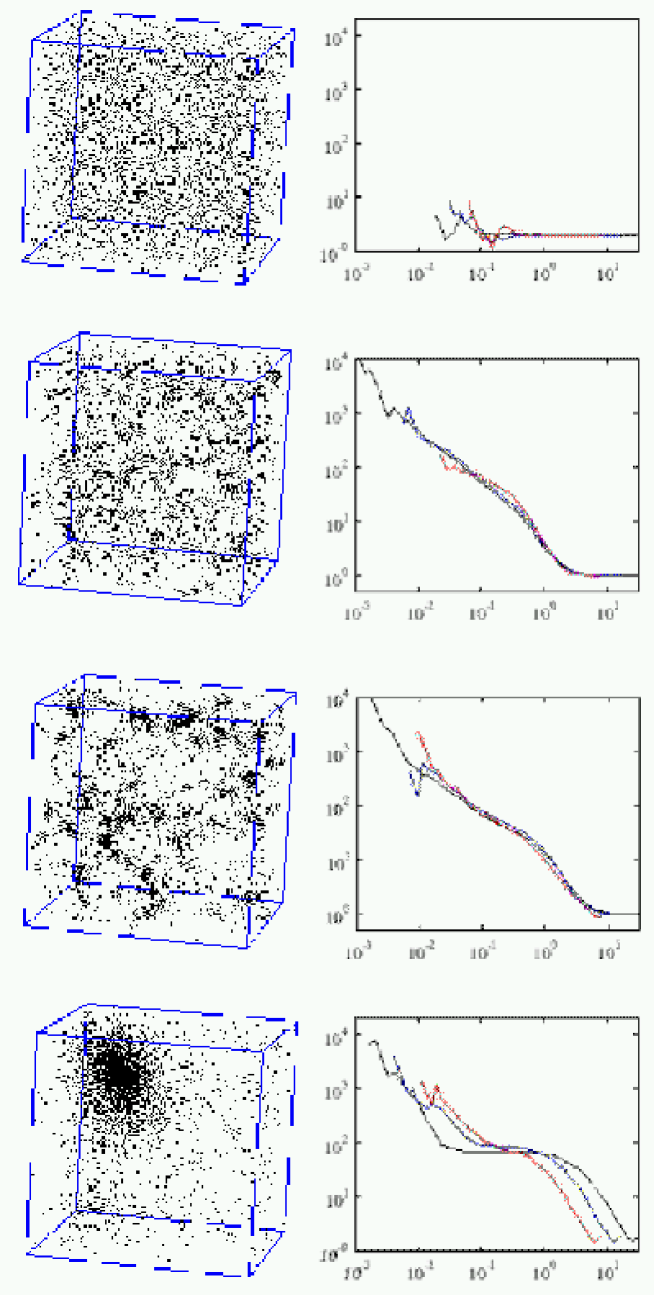
Figure 1: Evolution of particle positions for a simulation with $32^{3}$ particles (left column) and the corresponding measure of $\Gamma^{*}$ (right column). The three lines correspond to the $\Gamma^{*}$ for simulations with $N=8^{3}$, $N=16^{3}$, $N=32^{3}$ particles.

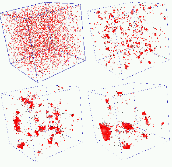
Figure 2: Evolution of particle positions for a simulation with $32^{3}$ particles.

We run a series of simulations with $N=8^{3}$, $N=16^{3}$, $N=32^{3}$. The evolution of the positions of the particles for the $N=32^{3}$ simulation is shown in the left column of figure 1. At the initial time the system is set with a homogeneous density and no velocities. After a while, clusters begin to form at small scales, while at large scales the distribution is still homogeneous. As the evolution goes on, clustering extends to larger and larger scales, up to the size of the simulation box. In the final stage of the system almost all the particles belong to a single cluster. This state is stationary.

In figure 1 we show the evolution of particle positions (left column) together with the corresponding measures of spatial correlations, performed with $\Gamma^{*}$ (right column). The three lines correspond to the results for the aforementioned three simulations. An important consideration is that the correlation properties are the same for systems with different number of particles. This is true for the intermediate states of the evolution, of which we show two snapshots at different times in the central rows of fig.1. On the contrary, this is not true for the last row, which corresponds to the final, stationary state of the systems.

We can interpret such results by saying that the intermediate stages of the evolution show a well defined thermodynamic limit, that is, the correlation properties at a fixed time are the same as $N\rightarrow\infty$, keeping $N/V=const$. This property can be understood by noting that the effective range of the gravitational interaction is finite.

This seems to be in contradiction with the long range nature of the interaction. However, the reason lies in the long range isotropy of the initial conditions.

4 The Holtsmark distribution

The distribution of the forces acting on a particle in an infinite Poisson system can be derived exactly [15], [16]. The starting point is to consider the probability of having a force $F$ on a particle due to all the $N$ particles in a sphere centered on it. Such probability can be expressed as:

$$W_{N}({\bf F})=\int d^{3}\,x_{1}\ldots d^{3}\,x_{N}\,p({\bf x_{1}})\ldots p({\bf x_{N}})\delta({\bf F}-\sum_{i=1}^{N}{\bf F(x_{i})})$$ (3)

where $p({\bf x_{i}})=3/(4\pi\,R^{3}))$ is the probability to have particle $i$ in ${\bf x_{i}}$. In the equation (3), it has been possible to write the $N$ point probability as the product of $N$ independent one-point probabilities, because the point distribution is Poissonian. The dirac $\delta$ can be now expressed in its Fourier representation. This allows to reduce the previous integral to:

$$W_{N}({\bf F})=\left(\frac{1}{2\pi}\right)^{3}\int exp(-i{\bf k}\cdot{\bf F})A({\bf k})\,d^{3}k$$ (4)

where:

$$A({\bf k})=\left[\int exp(i{\bf k}\cdot{\bf F(x)})p({\bf x})d^{3}x\right]^{N}$$ (5)

and the last integral extends over the sphere. Expressing $N$ as $N=4\pi R^{3}n/3$, where $n$ is the average density in the system, and taking the limit $R\rightarrow\infty$ and $n=const$ $A({\bf k})$ becomes:

$$A({\bf k})=\exp(-nC({\bf k}))$$ (6)

where

$$C({\bf k})=\int_{|{\bf r}|}^{+\infty}d^{3}r(1-\exp({i{\bf k}\cdot{\bf F(r)}})$$ (7)

After some algebra we eventually get Holtsmark distribution:

$$W(F)=\frac{2}{\pi F}\int_{0}^{\infty}dx\;\exp[-(x/\beta)^{\frac{3}{2}}]\;x\;\sin(x)\;$$ (8)

where $\beta=F/F_{o}$ is an adimensional force and $F_{o}=\left[2\pi(4/15)^{2/3}\right]Gm/\lambda^{2}$. In the latter expression, $\lambda$ is the average inter-particle separation $=(V/N)^{1/3}$. In the limit $F\rightarrow\infty$, the equation (8) can be written as:

$$W(F)=\frac{2}{\pi F}Im\int_{0}^{\infty}xe^{ix}\left[1-(x/\beta)^{\frac{3}{2}}+\ldots\right]dx$$ (9)

Performing a suitable change of variables and retaining only the dominant terms, we get:

$$\lim_{F\to+\infty}W(F)=\frac{15}{8}\left(\frac{2}{\pi}\right)^{1/2}\frac{1}{F_{0}}\beta^{-5/2}=2\pi n\left(Gm\right)^{3/2}F^{-5/2}$$ (10)

On the hand, it is simple to compute the distribution of the forces $W_{nn}(F)$ on a particle due to its nearest neighbour in a Poisson distribution. Actually, in this case:

$$W_{nn}(F)dF=\omega(r)dr$$ (11)

where $\omega(r)=4\pi r^{2}\,exp(-4\pi r^{3}n/3)$ is the probability to find the nearest neighbour of a particle at a distance $r$ from it. From the previous equation we get:

$$W_{nn}(F)=4\pi r^{2}n\cdot\exp(-4\pi r^{3}n/3)\left(\frac{dF}{dr}\right)^{-1}$$ (12)

which can be easily solved:

$$W_{nn}(F)=2\pi n\cdot(Gm)^{3/2}F^{-5/2}\exp\left[-4\pi n/3\cdot\left(Gm\right)^{3/2}F^{-3/2}\right]$$ (13)

In the limit $F\rightarrow\infty$ (i.e. $r<<\lambda$) the solution is simple:

$$W_{nn}(F)\approx 2\pi n\cdot(Gm)^{3/2}F^{-5/2}$$ (14)

The two expressions (10) and (14) are actually identical. This implies that the largest forces on the particles of the system are those due to the nearest neighbours. Particles quite isolated with respect to any another in the system are instead submitted to a force which comes from the interaction with a large number of particles

5 A qualitative model

At the beginning, the first particles to move are those which experience the largest forces. As we have seen, when the initial point distribution is poissonian, such particles are those with a neighbour closer than the average. The dynamics in this stage is then dominated by interactions on the scale of the nearest neighbours. In this sense the gravitational interaction at this stage has a finite effective range. This two-body interaction breaks the initial isotropy on a scale slightly larger than the mean inter-particle distance, while on large scales the system is still isotropic. Therefore, it is reasonable to argue that the dynamics we have described will act on this new scale.

The relevant dynamics therefore takes place on the scale on which the system is anisotropic. Once the particles have clustered on a scale, the isotropy is broken on a larger scales. Therefore, considerations similar to those developed for the scale of particles hold at subsequent times on larger scales, and it appears that the relevant forces are due to mass clumps present on such scales, while at very large scale the system is still isotropic. In this view long range interactions can be treated as interaction acting on a short range which increases with time.

In such a sense, gravitational dynamics proceeds from small to large scales by a transfer of discreteness from small to large scales.

When such scale is of the order of the simulation box, the evolution is dominated by finite size effects. Indeed, the particles are grouped only in few clusters and the existence of periodic boundary conditions, which prevent more particle to enter the simulation volume, forces the system toward a stationary state. As a consequence, for a system with a larger number of particles such finite size effects would take place at a later time, and therefore on a larger scale, as can be seen in the last row of figure 1. Here, the rightmost line is related to the simulation with $N=32^{3}$ particles, the leftmost line to the simulation with $N=8^{3}$.

Our description of the clustering is based on the discrete nature of the system. It is very interesting to notice that in this model the evolution of a system with long range interaction can be described in terms of a series of short range processes, which act on a progressively increasing scale. We argue that this argument could allow to describe the evolution of a true infinite self gravitating system at any time.

An important consideration which arises from this discussion is that this model of evolution depends on the statistical properties of the initial conditions. It applies to systems which are isotropic on large scales and anisotropic on small scales. On the contrary, for example, a typical initial condition used in cosmological simulations is a glass like distribution of particles, with large scale density fluctuations superimpose. In this case, the system is isotropic (regular) even on the smaller scales, so the dynamics is essentially driven by large scale fluctuations.

We take inspiration from renormalization to attempt to model the dynamics. The basic idea is that the relevant elements for the dynamics at a given time are the typical discrete objects formed at that time, i.e. clusters. We take the clusters to be structureless elements, and represent them with their total mass and their center of mass quantities. Fig. 2 can help in imagining the system in this approximation. Now we can repeat the argument we made for particles to such elements, which we can take to be a sort of macro particles. Of course there is no exact analytic expression for the force distribution at this scale; it is reasonable however to assume the the nearest macro particle will be most important for the dynamics of a given cluster.

We can modelize the system at any time as made of almost independent pairs of macropartices, and assume that the relevant dynamics can be described in such a way.

Visual inspection of the evolution of the system (fig. 2) suggests that clusters formed at a given time are the new discrete elements for the iteration of the clustering process at a larger scale.

However, this model is based on a strong assumption, i.e. that the clustering on a scales activates after the clustering on smaller scales. Of course this cannot be strictly true in general, since there are forces acting between overdensities before clusters form on a scale. We assume nevertheless that such forces are much smaller than those due to discreteness, so that the force due to it dominates the dynamics after some time.

In [17] we have illustrated this model in greater detail, giving a qualitative estimate for the growth rate of the clustering process.

6 A $1-d$ cellular automaton model

As we have discussed in previous chapter, the evolution of a random distribution of gravitationally interacting mass points can be described by nearest-neighbours interactions taking place at increasingly larger scales. This simplification is possible because the system is reasonably isotropic on scales larger than the scale of clustering. To understand in greater detail the dynamics due to a nearest neighbour interaction, we have investigated an extremely simple one-dimensional model.

We randomly distribute $10^{5}$ particles, of equal mass, on a line (of length $10^{5}$ units in our simulation), rather than on discrete lattice points as is the convention in cellular automata, and impose periodic boundary conditions. Particles move toward their nearest neighbours either by one unit at each time step or by half their separations from their nearest neighbours, whichever is shorter. If two particles are closer than a lower threshold, and in addition are mutual nearest neighbours, they coalesce at the mid-point of their separation, conserving mass. If a particle is equidistant from its left and right neighbours, which is an extremely rare event, it moves towards the right one.

Therefore this model focuses precisely on the rôle of granularity and self-similarity and leads to a schematic picture for the gravitational clustering phenomenon. One of the main differences between this model and most existing aggregation models such as DLA, Smoluchoski or 1-dimensional Burgers, is that its dynamics depends only on the positions and not on the masses and initial velocities of the aggregates.

Our model suggests a simple interpretation for the non-analytic hierarchical clustering and can reproduce the self-similar features of the real gravitational N-body simulations for white noise initial conditions.

Figure 3: The figure shows the trajectories of particles taken from a typical run of our simulation. The space-time tree is reminiscent of river networks in two-dimensional space and exhibits the property of topological scaling, a concept which is relevant for branched structures and originally arose as a means of analysing river networks.

The trajectories in space-time of the aggregates are shown in fig.(3). They show a tree-like topology. The tree structure of the aggregation process in space-time is a manifestation of topological self-similarity [18], which is a property of many branched structures such as river-networks and bronchial trees [19] and can be quantified by various scaling exponents, a most common of which is the Strahler index. For our model, this index has a value of $2$, as in Cayley tree structures [20].

Topological scaling is believed to emerge from a self-similar growth process. An appropriate way to analyse dynamical scaling is to study the mass distribution function $n(m,t)$, that is the fraction of aggregates of mass $m$ at time $t$. The results of the measures of $n(m,t)$ at different times $t$ are shown in fig.(4) as a function of $m/t$. We have found, by observing various scaling behaviours of our model [21], that the mass distribution function has the self-similar form

$$t^{2}\cdot n(m,t)=\left({m\over t}\right)^{3}e^{-(m/t)^{2}}$$ (15)

as is shown in figure 4.

The $t^{2}$ factor is a direct consequence of the mass conservation requirement of our model.

Figure 4: For more than two decades in time scale, the mass distribution obtained from our simulation shows a power-law behaviour at the low-mass end followed by a sharp exponential cut-off at the large-mass end, similar to Press-Schechter mass function which is commonly observed for real astrophysical data and cosmological N-body simulations. This selfsimilar distribution function indicate an underlying scale-invariant dynamics.

We have also analysed the density-density correlation for our model which develops a power law with exponent $-1$, followed by a flat behaviour. In 1 dimension an exponent $-1$ implies single objects (or dimension 0) followed by a smooth distribution. In this respect, the power-law behaviour of the correlation does not signal a fractal measure. In this model, unlike in fractal structures, large and small scales for mass and void distribution do not coexist, since the large mass particles are formed by the destruction of the substructures. Hence, the increase in correlation length is basically determined by the separations of the nearest neighbours and since these distances grow linearly with time, so does the correlation length.

We mainly focus on the universal features of the distribution of the masses of the aggregates and compare the self-similar features of such a function with that of Press-Schechter frequently encounters in astrophysics [22]. Press-Schechter mass function is a manifestation of the self-similar nature of gravitational hierarchical structure formation and has shown impressive agreements with simulations and observational results [22]. Although the cellular automata presented here gives rise to a mass function similar in some respect to Press-Schechter, it does not have the same exponents for white noise initial conditions. As compared to Press-Schechter distribution, here, small masses deplete rather fast and while they die out more massive objects do not form fast enough for the mass function to have a power-law decay for the small masses.

References

- [1] Davis M., in Critical dialogues in Cosmology, ed. Turok N., Word Scientific, Singapore (astro-ph/9611197) (1997)
- [2] Wu K. K. S., Lahav O. and Rees M., Nature 397, 225 (1999).
- [3] Totsuji H and Kihara T 1969 Publ. Astron. Soc. Jap. 21 221
- [4] Peebles P. J. E., The Large Scale Structure of the Universe Princeton Universe Press (1980)
- [5] Coleman P. H. and Pietronero L., Phys. Rep. 213, 311 (1992).
- [6] Sylos Labini F., Montuori M. and Pietronero L., Phys. Rep. 293, 61 (1998).
- [7] Jeans J. H., Phil. Trans. A199 1 (1902)
- [8] Gabrielli A, Sylos Labini F and Pellegrini S 1999 Europhys. Lett.46 127
- [9] Capuzzo Dolcetta R and Miocchi P. 1998 J. Comp. Phys. 143,29
- [10] Springel V, Yoshida N and White S D M New Astronomy 6, 58 (2000).
- [11] Ewald P. P.Ann. Physik64 253 (1921)
- [12] L. Hernquist, N. Katz, 1989,Ap. J. S.,70, 419
- [13] Baertschiger T. and Sylos Labini F., Europhys. Lett., in print (2001)
- [14] Kuhlman B, Melott A L, and Shandarin S,Astrophysical Journal Letters470, L41 (1996).
- [15] Holtsmark J., Ann. d. Phys.58 577 (1917)
- [16] S. Chandrasekhar, Rev. Mod. Phys. 15, 1 (1943).
- [17] Bottaccio M., Amici A., Miocchi P., Capuzzo Dolcetta R., Montuori M. and Pietronero L. Europhys. Lett., in print (2001)
- [18] T. C. Halsey, Physics Today 53, 36 (2000).
- [19] I. Rodríguez-Iturbe and A. Rinaldo, Fractal river basins, Chance and Self-rganization (CUP, Cambridge 1997).
- [20] G. Caldarelli, R. Marchetti and L. Pietronero, Euro. Phys. Lett. 52, 386 (2000).
- [21] Roya Mohayaee and Luciano Pietronero, A cellular automaton model of gravitational structure formation, Preprint (2001).
- [22] W. H. Press and P. Schechter, Astro. Phys. J. 187, 425 (1974).