Quantum transport through mesoscopic disordered interfaces, junctions, and multilayers

Abstract

The study explores perpendicular transport through macroscopically inhomogeneous three-dimensional disordered conductors using mesoscopic methods (real-space Green function technique in a two-probe measuring geometry). The nanoscale samples (containing $\sim 1000$ atoms) are modeled by a tight-binding Hamiltonian on a simple cubic lattice where disorder is introduced in the on-site potential energy. I compute the transport properties of: disordered metallic junctions formed by concatenating two homogenous samples with different kinds of microscopic disorder, a single strongly disordered interface, and multilayers composed of such interfaces and homogeneous layers characterized by different strength of the same type of microscopic disorder. This allows us to: contrast resistor model (semiclassical) approach with fully quantum description of dirty mesoscopic multilayers; study the transmission properties of dirty interfaces (where Schep-Bauer distribution of transmission eigenvalues is confirmed for single interface, as well as for the stack of such interfaces that is thinner than the localization length); and elucidate the effect of coupling to ideal leads (“measuring apparatus”) on the conductance of both bulk conductors and dirty interfaces When multilayer contains a ballistic layer in between two interfaces, its disorder-averaged conductance oscillates as a function of Fermi energy. I also address some fundamental issues in quantum transport theory—the relationship between Kubo formula in exact state representation and “mesoscopic Kubo formula” (which gives the zero-temperature conductance of a finite-size sample attached to two semi-infinite ideal leads) is thoroughly reexamined by comparing their answers for both the junctions and homogeneous samples.

I Introduction

The experimental discovery [1, 2] of a giant magnetoresistance (GMR) phenomenon has revived interest in the transport properties of macroscopically inhomogeneous conductors, such as metallic junctions [3] or multilayers. [4] Furthermore, unusual systems for traditional transport theory, like single dirty interface [5] which are ubiquitous elements in such circuits, have entailed the introduction of new concepts to replace usual quantities (e.g., mean free path $\ell$) used to describe transport in bulk samples. Although some of these problems were formulated long ago within the (semiclassical) transport theory, [6, 7, 8] new attacks have employed all (quantum and semiclassical) transport formalisms developed thus far revealing that such problems are by no means resolved. [4, 9] In particular, the reexamination of various fundamental issues in the transport theory has been brought about by the experimental and theoretical advances in mesoscopic physics. [10] Thus, the Landauer-Büttiker scattering formalism [11] has been frequently invoked to study transport in both non-magnetic [12] and magnetic multilayered conductors. [13, 14] Obviously, the thorough understanding of transport properties due to purely multilayer + disorder effects is prerequisite for the analysis of more complicated phenomena in inhomogeneous structures.

Besides providing the means to compute the (quantum) conductance of finite-size samples, mesoscopic methods give additional physical insight by delineating transmission properties of the sample (note that one can technically treat transport in macroscopic samples without really using such fully quantum-mechanical transport theories [4]). The finite-size of mesoscopic systems play an important role in determining the conductance through scattering approach, but no further limitations exist—the exactness of results obtained in this guise is heavily exploited in throughout the paper. Practical realization of this program appears in different incarnations, i.e., different Landauer-type [15] or Kubo [16] formulas for a finite-size phase-coherent sample attached to semi-infinite ideal (i.e., disorder-free) leads. These prescriptions are usually made computationally efficient by combining them with some Green function technique. [17, 18]

Here I employ mesoscopic quantum transport methods to calculate the conductance of disordered samples which are macroscopically inhomogeneous, i.e., composed of different homogeneous conductors (“layers”) joined through some interfaces (“monoatomic layers”). In homogeneous conductors, whose properties are well-studied throughout the history of localization theory, [19] impurities generate only microscopic inhomogeneity on the scale $\sim\lambda_{F}$ (Fermi wavelength). Our goal is twofold: (1) Most mesoscopic studies have been focused on the bulk homogeneous conductors [18] in the weak scattering transport regime. Only recently the systems like metallic multilayers, [12] or single dirty interfaces [5, 20] have been tackled in this guise. By employing nonperturbative numerical methods we can access strongly disordered junctions, single strongly disordered interface (when stacked together to form a bulk conductor our interfaces would form an Anderson insulator), and multilayers composed of such interfaces and bulk diffusive or ballistic mesoscopic conductors. A system is called mesoscopic if its size $L$ is smaller than the dephasing length $L_{\phi}$, which is a typical distance for electron to travel without loosing its phase coherence ($L_{\phi}\lesssim 1\,\mu$m in current low-temperature experiments), and is therefore determined by decoherence processes caused by the coupling to environment either through inelastic scattering (electron-electron and electron-phonon) or just be the change of the environment quantum state (e.g., spin-flip scattering from a magnetic impurity). The term metallic implies that conductance $G$ of a bulk homogeneous sample is much larger than the conductance quantum $G_{Q}=2e^{2}/h$. For interfaces one needs a different nomenclature: they are termed “dirty” [5] if their conductance $G/G_{Q}$ is much smaller than the number of conducting channels $N_{\rm ch}$ ($N_{\rm ch}\sim k_{F}^{2}S$ in three-dimensions, with $k_{F}=2\pi/\lambda_{F}$, and $S$ is the cross section of a sample). Lacking a better language, I denote the multilayers studied here as “dirty metallic”, meaning that scattering is due to a random potential and their conductance is $G_{M}\ll G_{Q}N_{\rm ch}$. Nevertheless, layer components are chosen to be metallic $G\gg G_{Q}$, and are well-described, in the diffusive limit $L\gg\ell$, by semiclassical transport theory. [21] In terms of material parameters, the resistivity of a bulk homogeneous material, from which nanoscopic layers are cut out, is few $100\,\mu\Omega$cm, which is typical of dirty transition metal alloys. Thus, the possible small conductance of layers is not necessarily caused by approaching the localization-delocalization transition [22] upon increasing disorder, as is usual in the homogeneous bulk samples. The conductors are modeled by a tight-binding Hamiltonian with on-site potential disorder. This corresponds to a model of free electrons (understood here as Landau quasiparticles with parameters renormalized by both band structure effects and Fermi liquid interaction) with random point scatterers, [9] which is used frequently in studies of similar systems. While isotropic scattering sets semiclassical vertex corrections to zero (which are determined by ladder diagrams [23] generating difference between momentum relaxation time and elastic mean free time, or scattering-in term in the Boltzmann theory), it does not eliminate the higher order quantum interference vertex corrections. These terms are nonlocal on the mesoscopic length scale $L_{\phi}$, and therefore invalidate [4] the concept of local position dependent conductivity $\sigma(x)$ as usual way of describing the multilayered structures (in semiclassical approximation). [9] Since I exploit here exact techniques, all quantum localization effects which are not necessarily small in dirty systems, [9, 21] are included from the onset. All three types of samples are studied for electron transport perpendicular to the layers (or interfaces), which is the so-called current perpendicular to plane (CPP) geometry. [4] Once the disorder-averaged resistance of the multilayer is computed, we can compare it to the resistance given by the resistor model, [24] (i.e., a sum of the bulk layers and interface resistances connected like classical Ohmic resistors in a series). (2) I investigate some fundamental issues in the quantum transport theory using dirty metallic junctions from above as a testing ground, as well as homogeneous disordered samples as a reference. That is, I compare the transport properties computed from the Kubo formula in exact single particle state representation (which was widely used [25] in the “premesoscopic” era [26] of the Anderson localization theory) and “mesoscopic Kubo formula” for the open finite-size system attached to two ideal leads. [16] In the former case the system is closed and the eigenproblem of the Hamiltonian is solved exactly by numerical diagonalization, while in the latter case energy levels of a sample are broadened by the coupling to the leads, and I use real-space Green functions for such open sample plugged into the Kubo formula [16] (which is then equivalent to the Landauer two-probe formula [27]) to get its conductance. Also, the influence of the leads (“measuring apparatus”) and the lead-sample coupling on the conductance (which is akin to the problems encountered in quantum measurement theory [28]) is explicitly quantified.

The paper is organized as follows. The first Sec. II deals with some general remarks on the Kubo linear response formalism and current conservation. This should serve as a guidance for proper application of Kubo formulas on the finite-size systems. In Sec. III, the Kubo formula in exact state representation is compared to the Kubo formula for the finite-size sample by evaluating them for dirty metallic junction, as well as for homogeneous samples. Section IV presents the results on the transmission properties, and conductance derived from them, of a single dirty interface as well as thin layers composed of few of such interfaces. The calculations are completed in Sec. V by examining different types of multilayers, containing disordered and/or ballistic layers concatenated through interfaces from Sec. IV. Section VI provides a summary of the technical, emphasizing physical insights gained from them.

II Kubo formulas and current conservation

The basic global transport property, for small applied voltage, is linear conductance (or equivalent resistance $R=1/G$). The conductance $G$ is defined by the Ohm’s law

$$I=G\,V,$$ (1)

relating the current $I$ to the voltage drop $V$. Since this is a plausible relation for a linear transport regime, more information is contained in the local form of the Ohm’s law

$${\bf j}(\bf{r},\omega)=\int\!d{\bf r}^{\prime}\,\mbox{\@text@baccent{$\sigma$}}({\bf r},{\bf r}^{\prime};\omega)\cdot{\bf E}({\bf r}^{\prime},\omega).$$ (2)

In what follows, the focus will be on the DC transport $\omega\rightarrow 0$. Although it is possible to treat ${\bf E}({\bf r})$ as an externally applied electric field and then include the effects of Coulomb interaction between electrons as a contribution to the vertex correction, [4] the usual approach is to use the total (local and inhomogeneous) electric field ${\bf E}({\bf r})\equiv{\bf E}_{\rm loc}({\bf r})=-\nabla\mu({\bf r})/e$, which is the sum of external field plus the field due to the charge redistribution from the system response. [47] The electrons are then treated as independent quasiparticles. The electrochemical potential $\mu$ in non-equilibrium situations (like transport) is not a well-defined quantity, and can serve only e.g., to parameterize the carrier population. [29] The relation (2) defines the meaning of the nonlocal conductivity tensor (NLCT) $\mbox{\@text@baccent{$\sigma$}}({\bf r},{\bf r}^{\prime})$ as the fundamental microscopic quantity in the linear response theory. This quantity gives the current response at ${\bf r}$ due to an electric field at ${\bf r}^{\prime}$. The requirement of current conservation in the DC transport

$$\nabla\cdot{\bf j}({\bf r})=0,$$ (3)

coupled to Eq. (2) and together with appropriate boundary conditions at the infinity or possible interfaces, [30] makes it possible to find ${\bf E}({\bf r})$. The conductance (dissipated power by the voltage $V$ squared) is then given by

$$G = \frac{1}{V^{2}}\int\limits_{\Omega}d{\bf r}\,{\bf E}({\bf r})\cdot{\bf j}({\bf r})$$ (4)

$$= \frac{1}{V^{2}}\int\limits_{\Omega}d{\bf r}\,d{\bf r}^{\prime}\,{\bf E}({\bf r})\cdot\mbox{\@text@baccent{$\sigma$}}({\bf r},{\bf r}^{\prime})\cdot{\bf E}({\bf r}^{\prime}),$$ (5)

where $\Omega$ is the sample volume, and at first sight requires the knowledge of local electric fields within the sample. However, it was shown in the course of recent reexamination of transport theory, [31] driven by the problems of mesoscopics, that current conservation imposes stringent requirements on the form of NLCT

$$\nabla\cdot\mbox{\@text@baccent{$\sigma$}}({\bf r},{\bf r}^{\prime})=\mbox{\@text@baccent{$\sigma$}}({\bf r},{\bf r}^{\prime})\cdot\nabla^{\prime}=0,$$ (6)

where absence of magnetic field is assumed to get this special case of a more general theorem. [27] This allows us to use arbitrary electric field factors in Eq. (4), including ${\bf E}({\bf r})\neq{\bf E}({\bf r}^{\prime})$ [a homogenous field $E=V/L$ is usually implied in the textbook literature [23]].

When a finite-size sample is attached to two semi-infinite ideal leads, the condition (6) is sufficient to show that [27]

$$G=-\int\limits_{S_{1}}\!\int\limits_{S_{2}}d{\bf S}_{1}\cdot\mbox{\@text@baccent{$\sigma$}}({\bf r},{\bf r}^{\prime})\cdot d{\bf S}_{2},$$ (7)

by using the divergence theorem to push the integration from the bulk onto the boundary surface [32] going through the leads and around the disordered sample (the integration over this insulating boundary obviously gives zero contribution because no current flows out of it). The surface integration in the two-probe conductance formula (7) is over surfaces $S_{1}$ and $S_{2}$ separating the leads from the disordered sample. The vectors $d{\bf S}_{1}$ and $d{\bf S}_{2}$ are normal to the cross sections of the leads, and are directed outwards from the region encompassed by the overall surface (composed of $S_{1}$, $S_{2}$ and insulating boundaries of the sample). It is assumed that voltage in one of the leads is zero, e.g., $\mu_{L}=0$ and $\mu_{R}=eV$. The meaning of current conservation and expression (7) is quite transparent—current $I$ at a given cross section depends only on the voltages in the leads (in experiment one either fixes this voltages by a voltage source, or fixes the current by a current source) and not on the precise electric field configurations. The formula (7) can be generalized [27] to arbitrary multi-probe geometry, while the volume-averaged conductance (4) is meaningful only for the two-probe measurement. The expression (7) is valid even in the presence of interactions, where many-body effects can be introduced using Kubo formalism to get $\mbox{\@text@baccent{$\sigma$}}({\bf r},{\bf r}^{\prime})$ microscopically. However, this route is tractable and useful especially in the case of noninteracting quasiparticle systems. When a sample is attached to ideal leads (see below), this established rigorous equivalence [27] between two different linear response formulations—Kubo and Landauer-Büttiker [11] (to work out the proof, $S_{1}$ and $S_{2}$ should be placed far enough into the leads so that all evanescent modes from the sample have died out and do not contribute to the conductance [4]). In the scattering approach to transport, pioneered by Landauer through heuristic and subtle arguments, the conductance of a noninteracting system is then expressed in terms of the transmissions probabilities between different quantized transverse propagating modes defined by the leads as asymptotic scattering states [see Eq. (11)].

Although Boltzmann formalism can provide semiclassical expression for NLCT (which is nonlocal on the scale of the sample size because of the classical requirement of current conservation [33]), the standard quantum route to it is the Kubo linear response theory (KLRT). Linear response theory gives a full quantum description of transport (i.e., it includes quantum interference effects in the motion of electrons [34]) in non-equilibrium systems that are still close enough to equilibrium for vanishingly small applied external electric field. [35] Therefore, the formulas above involve the equilibrium expectation values of the corresponding quantum-mechanical operators, in accordance with fluctuation-dissipation theorem underlying KLRT [e.g., it is assumed that ${\bf j}(\bf{r})$ is the expectation value of the current density operator in the quantum formalism]. While the current is response to the total electric field (external + induced), the NLCT is obtained as a response to the external field only [36, 37] because the current induced by the external field is already linear in the field. Therefore, in the linear response one does not need the corrections due to induced non-equilibrium charges (electron-electron interaction is taken in the equilibrium, e.g. through renormalized parameters of the Landau quasiparticles and the self-consistent screening effect on the impurity scattering).

Since Kubo NLCT is not experimentally measurable quantity, macroscopic conductivity $\sigma$ is obtained by volume averaging NLCT through Eq. (4) where $\sigma=G\,L/S$ for a cubic sample of length $L$ and cross section $S$ (limit $\Omega=LS\rightarrow\infty$ is assumed, while keeping the impurity concentration finite). This usually implies a homogeneous ${\bf E}({\bf r})$ factors, which is justified by the fact that Kubo expression for NLCT is divergenceless (as can be easily proven [31] from its current-current correlation form, [23]) i.e., it satisfies Eq. (6). Thus, the volume-averaged conductivity $\sigma$ relates the spatially averaged current ${\bf j}=\int d{\bf r}\,{\bf j}({\bf r})/\Omega$ to the spatially-averaged electric field,

$${\bf j}=\sigma{\bf E}.$$ (8)

For a noninteracting system of fermions this leads to a Kubo formula in exact single-particle state representation (KFESR)

$$\sigma_{xx} = \frac{2\pi\hbar e^{2}}{\Omega}\sum_{\alpha,\,\alpha^{\prime}}|\langle\alpha|\hat{v}_{x}|\alpha^{\prime}\rangle|^{2}$$ (10)

$$\times\delta(E_{\alpha}-E_{F})\delta(E_{\alpha^{\prime}}-E_{F}),$$

where the factor of two for spin degeneracy will be explicit in all formulas. The delta functions in Eq. (10) emphasize that conductivity is a Fermi surface ($E_{F}$ is the Fermi energy) property at low temperatures [$T\rightarrow 0\Rightarrow-\partial f(E)/\partial E\simeq\delta(E_{F}-E)$, $f(E)$ being the Fermi-Dirac distribution function]. Here $\hat{v}_{x}$ is the $x$-component of the velocity operator and $|\alpha\rangle$ are eigenstates of a single-particle Hamiltonian, $\hat{H}|\alpha\rangle=E_{\alpha}|\alpha\rangle$. The velocity operator $\hat{\bf v}$ is determined through the equation of motion for the position operator $\hat{\bf r}$

$$i\hbar\hat{{\bf v}}=i\hbar\frac{d\hat{{\bf r}}}{dt}=[\hat{{\bf r}},\hat{H}],$$ (11)

where $\hat{H}$ is the Hamiltonian before the application of the external electric field (in the spirit of FDT).

In the general case, conductivity is a tensor, but since symmetries are restored after disorder-averaging, one can use $\sigma=(\sigma_{xx}+\sigma_{yy}+\sigma_{zz})/3$ as the scalar conductivity. This is valid only in the case of homogenously disordered sample. For example, in our metal junction or multilayers $\sigma_{xx}$ is different from $\sigma_{yy}$ and $\sigma_{zz}$. To get the conductivity (as an intensive quantity) in KLRT, the thermodynamic limit $\Omega$ is always understood (no stationary regime can be reached in a system which in neither infinite nor coupled to some thermostat). In the disorder electron physics this also bypasses the ambiguity of conductivity which scales [38] with the length of the system (although scaling is unimportant [22] in the metallic regime $G\gg G_{Q}$). Nonetheless, the computation of transport properties from exact single particle eigenstates, obtained by the numerical diagonalization of Hamiltonian of a finite-size system, has been frequently employed in the development of disordered electron physics. [25] In fact, it is still the standard method for computing the conductivity of many-body systems by diagonalizing small clusters of some lattice fermion Hamiltonian. [39] However, direct application of the formula (10) leads to a trouble since eigenvalues are discrete when the sample is finite and isolated. Strictly speaking, the conductivity is then a sum of delta functions, and to obtain finite conductivity they have to be broadened into functions having a finite width larger than the level spacing. Thus, there are two numerical tricks which can be used to “circumvent” this problem: (i) one can start from the Kubo formula for the frequency dependent conductivity

$$\sigma_{xx}(\omega) = \frac{2\pi\hbar e^{2}}{\Omega}\sum_{\alpha,\,\alpha^{\prime}}|\langle\alpha|\hat{v}_{x}|\alpha^{\prime}\rangle|^{2}$$ (13)

$$\times\frac{f(E_{\alpha})-f(E_{\alpha^{\prime}})}{\hbar\omega}\delta(E_{\alpha}-E_{\alpha^{\prime}}-\hbar\omega),$$

average the result over finite $\omega$ values, and finally extrapolate [40] to the static limit $\omega\rightarrow 0$; (ii) The delta functions in Eq. (10) can be broadened into a Lorentzian

$$\delta(x)\rightarrow\bar{\delta}(x)=\frac{1}{\pi}\frac{(\eta/2)^{2}}{x^{2}+(\eta/2)^{2}},$$ (14)

where $\eta$ is the full width at half maximum of the Lorentzian. I find that both methods produce similar results. The calculations presented below use the broadened delta function $\bar{\delta}(x)$ in the formula for static Kubo conductivity.

FIG. 1.: A two-dimensional version of the actual 3D model used here for a two-probe measuring geometry. Each site hosts a single $s$-orbital which hops to six (or fewer for surface atoms) nearest neighbors. The hopping matrix element is $t$ (within the sample), $t_{\rm L}$ (within the leads), and $t_{\rm C}$ (coupling of the sample to the leads). The leads are semi-infinite and connected smoothly at $\pm\infty$ to macroscopic reservoirs biased by the chemical potential difference $\mu_{L}-\mu_{R}=eV$.

The Green operator of a noninteracting Hamiltonian (with specified boundary conditions),

$$\hat{G}^{r,a}=[E-\hat{H}\pm i\eta]^{-1},$$ (15)

contains the same information encoded in the single-particle wave function. Therefore, using the expansion of single-particle Green operator $\hat{G}^{r,a}=\sum_{\alpha}|\alpha\rangle\langle\alpha|/(E-E_{\alpha}\pm i\eta)$ in terms of exact eigenstates, the Kubo formula for the macroscopic (volume-averaged) longitudinal conductivity can be recast into the following expression [41]

$$\sigma_{xx} = \frac{2\pi e^{2}\hbar}{\Omega}\,\text{Tr}\left[\hat{v}_{x}\,\delta(E-\hat{H})\,\hat{v}_{x}\,\delta(E-\hat{H})\right],$$ (17)

$$\delta(E-\hat{H}) = -\frac{1}{\pi}\text{Im}\,\hat{G}=\frac{1}{2i}(\hat{G}^{r}-\hat{G}^{a}).$$ (18)

When employing this formula one faces the same problem as in the KFESR—in order to define [42] retarded ($r$) or advanced ($a$) Green function a small parameter $\eta\rightarrow 0^{+}$ requires numerical handling [43] analogous to the one (14) involved in the KFESR (10). However, it is possible to derive another, “mesoscopic Kubo formula”, for the finite-size sample attached to two semi-infinite clean leads. [27] This formula represent a fully quantum-mechanical expression for the zero-temperature conductance

$$G_{xx}=\frac{4e^{2}}{h}\frac{1}{L_{x}^{2}}\,{\rm Tr}\left(\hbar\hat{v}_{x}{\rm Im}\,\hat{G}\,\hbar\hat{v}_{x}{\rm Im}\,\hat{G}\right),$$ (19)

which, being measurable, is the only meaningful quantity to discuss in mesoscopics (the alternative is to introduce conductivity as the NLCT). Namely, in quantum-coherent samples ($L>L_{\phi}$) local description of transport in terms of conductivity breaks down because of the nonlocal correction (e.g., weak localization [44]) induced on the scale of $L_{\phi}\gg\ell$, which is much larger than the elastic mean free path. Thus, mesoscopic samples have to be treated as a single coherent unit (“giant molecule”), so that its conductance cannot be interpreted as a combination $G=\sigma A/L$ of the conductances of its parts (i.e., such description becomes applicable only at high enough temperatures). Although the formula (19) apparently looks like Eq. (15), the crucial difference is that the following Green operator is plugged there instead

$$\hat{G}^{r,a}=[E-\hat{H}-\hat{\Sigma}^{r,a}]^{-1}.$$ (20)

This change is not innocuous: $\hat{G}^{r}$ ($\hat{G}^{a}=[\hat{G}^{r}]^{\dagger}$, $\hat{\Sigma}^{a}=[\hat{\Sigma}^{r}]^{\dagger}$) has acquired a self-energy term from the “interaction” with the leads. [18] This looks like the self-energy term in the many-body Green functions, but this one is exactly calculable, as shown below. Thus, the leads enforce new boundary conditions. Since $\hat{\Sigma}^{r}(E)$ contains an imaginary part when energy $E$ belongs to the band of a lead, no small parameter $\eta$ is needed to define the retarded or advanced Green operator.

The lattice model of a two-probe measuring geometry, to be used in the subsequent sections for evaluation of Eq. (19), is shown in Fig. 1. The three-dimensional (3D) nanocrystal (“sample”) is placed between two ideal (disorder-free) semi-infinite “leads” which are connected smoothly to macroscopic reservoirs at infinity. The electrochemical potential difference $eV=\mu_{L}-\mu_{R}$, which drives the current, [45] is measured between the reservoirs. It is assumed that reservoirs inject thermalized electrons at electrochemical potential $\mu_{L}$ (from the left) or $\mu_{R}$ (from the right) into the system. All inelastic scattering occur in the reservoirs, which therefore ensure steady state transport in the central region. Semi-infinite leads [46] are a convenient method to take into account electrons entering of leaving the phase-coherent sample (i.e., effective Hamiltonian of an open system, $\hat{H}+\hat{\Sigma}^{r}$ in Eq. (20), is non-Hermitian). This makes it possible to bypass explicit modeling of thermodynamics of perfect (i.e., unaffected by the flow of current) macroscopic reservoirs which are introduced heuristically in the scattering approach (for a different interpretation of the role of perfectly conducting leads in the derivation of Kubo formula for a finite-size system see Ref. [47]). The leads have the same cross section as the sample, which eliminates scattering induced by the wide to narrow geometry at the sample-lead interface. [48] The whole system is described by the following Hamiltonian with nearest neighbor hopping integrals $t_{\bf mn}$

$$\hat{H}=\sum_{\bf m}\varepsilon_{\bf m}|{\bf m}\rangle\langle{\bf m}|+\sum_{\langle{\bf m},{\bf n}\rangle}t_{\bf mn}|{\bf m}\rangle\langle{\bf n}|.$$ (21)

where $\langle{\bf r}|{\bf m}\rangle$ is the $s$-orbital $\psi({\bf r}-{\bf m})$ located on site ${\bf m}$. The site representation, defined by the basis states $|{\bf m}\rangle$, can be interpreted either as a tight-binding description of electronic states or as discretization of corresponding single-particle Schrödinger equation. The sample is the central section with $N\times N_{y}\times N_{z}$ sites. The hopping in the sample set the unit of energy $t_{\bf mn}=t$. The disorder will be introduced by taking $\varepsilon_{\bf m}$ to be a random variable. The leads are clean ($\varepsilon_{\bf m}=0$) but, in general, have different hopping integrals $t_{\bf mn}=t_{\text{L}}\neq t$. Finally, the hopping which couples sample to the leads is $t_{\bf mn}=t_{\text{C}}$. Hard wall boundary conditions are set in the $\hat{y}$ and $\hat{z}$ directions. The different hopping integrals introduced here are necessary when studying disordered samples to get the conductance at Fermi energies throughout the whole band extended (compared to the clean case) by disorder, i.e., in such calculations one has to set $t_{\text{L}}>t$.

In site representation, Green operator $\hat{G}^{r,a}$ becomes a Green function matrix $\hat{G}^{r,a}({\bf n},{\bf m})=\langle{\bf n}|\hat{G}^{r,a}|{\bf m}\rangle$. The self-energy $\hat{\Sigma}^{r}=\hat{\Sigma}_{L}^{r}+\hat{\Sigma}_{R}^{r}$ “measures” the coupling of the sample to the leads. This causes the broadening of initially discrete levels and, thus, the finite lifetime of electron in the sample. Since electron which leaves the sample does not return phase-coherently, the dephasing length is by definition $L_{\phi}=L_{x}$. Each lead generates its self-energy term which has nonzero matrix elements only on the edge layers of the sample which are adjacent to the leads. They are defined as

$$\hat{\Sigma}^{r}_{L,R}({\bf n},{\bf m})=t_{\text{C}}^{2}\hat{g}_{L,R}^{r}({\bf n}_{S},{\bf m}_{S}),$$ (22)

with $\hat{g}_{L,R}^{r}({\bf n}_{S},{\bf m}_{S})$ being the surface Green function of a bare semi-infinite lead between the sites ${\bf n}_{S}$ and ${\bf m}_{S}$ in the end atomic layer of the lead [18] (adjacent to the corresponding sites ${\bf n}$ and ${\bf m}$ inside the conductor). I provide here explicit expression for these self-energy terms in the most general case when hopping integrals $t\neq t_{\text{C}}\neq t_{\text{L}}$ are different in different parts of the setup in Fig. 1

$$\hat{\Sigma}^{r}_{L,R}({\bf n},{\bf m}) = \frac{2}{N_{y}+1}\frac{2}{N_{z}+1}\sum_{k_{y},k_{z}}\sin(k_{y}n_{y}a)\sin(k_{z}n_{z}a)$$ (24)

$$\times\hat{\Sigma}^{r}(k_{y},k_{z})\sin(k_{y}m_{y}a)\sin(k_{z}m_{z}a).$$

This expression is obtained by expanding the surface Green function $\hat{g}_{L,R}^{r}({\bf n}_{S},{\bf m}_{S})$ in terms of exact eigenstates of the Hamiltonian of a semi-infinite lead, which satisfy

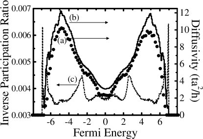
FIG. 2.: Diffusivity $\langle D_{x}(E_{F})\rangle$ of a disordered binary alloy modeled by a tight-binding Hamiltonian with quenched disorder ($\varepsilon_{A}=-2$ and $\varepsilon_{B}=2$) on a lattice $18\times 8\times 10$: (a) computed using the Kubo formula (19) in terms of the Green function for the sample with attached leads; (b) computed from the Kubo formula in exact single-particle eigenstate representation (29), where the width of the Lorentzian broadened delta function is $\eta=25\Delta(E_{F})$. Also plotted (c) is the IPR, defined in Eq. (31), which gives insight (i.e., degree of localization) into the structure of eigenstates used to evaluate the Kubo formula Eq. (29). The disorder averaging is performed over 50 samples.

particular hard wall transverse boundary conditions. Here $({\bf n},{\bf m})$ is the pair of sites on the surfaces inside the sample which are adjacent to the leads $L$ or $R$, in accordance with (22). Since electrons are confined in the $y$ and $z$ direction, electronic states in the lead have transverse wave function which are labeled by the discrete quantum numbers. They define subbands and corresponding conducting “channels” [i.e., transverse propagating modes as the product of transverse wave function and Bloch wave in the $x$-direction, $\langle{\bf m}|k_{y},k_{z}\rangle\otimes|k_{x}\rangle$], which represent a basis of scattering states for the scattering matrix of the disordered region, as envisaged in the Landauer picture of quantum transport. The self-energy $\hat{\Sigma}^{r}(k_{y},k_{z})$ of the channel $(k_{y},k_{z})$ is given by

$$\hat{\Sigma}^{r}(k_{y},k_{z})=\frac{t_{\text{C}}^{2}}{2t_{\text{L}}^{2}}\left(E_{\Sigma}-i\sqrt{4t_{\text{L}}^{2}-E_{\Sigma}^{2}}\right),$$ (25)

for $|E_{\Sigma}|<2t_{\text{L}}$. I use the shorthand notation $E_{\Sigma}=E-\varepsilon(k_{y},k_{z})$, where $\varepsilon(k_{y},k_{z})=2t_{\text{L}}[\cos(k_{y}a)+\cos(k_{z}a)]$ is the energy of quantized transverse levels in the lead. In the opposite case $|E_{\Sigma}|>2t_{\text{L}}$ we get

$$\hat{\Sigma}^{r}(k_{y},k_{z})=\frac{t_{\text{C}}^{2}}{2t_{\text{L}}^{2}}\left(E_{\Sigma}-\text{sgn}\,E_{\Sigma}\sqrt{E_{\Sigma}^{2}-4t_{\text{L}}^{2}}\right).$$ (26)

When the level spacing of the subbands is much smaller than $E_{F}$, the number of channels at $E_{F}$ is large and the finite-size model can describe a metal. The possibility to evaluate exactly these self-energies allows us to avoid the inversion of an infinite matrix which would formally give the Green function for the whole system [18] in Fig. 1. The real-space Green function technique described here, pioneered by Caroli et al. [15] long before official inception of mesoscopic physics, treats an infinite system with a continuous spectrum by evaluating only the Green function between the states inside the sample. This offers an alternative to handling a finite-size sample through periodic boundary conditions, whose discrete spectrum prevents a direct evaluation of the Kubo formulas (10) and (15). In general, the technical advantage of Green function techniques is that they can be used even when well-defined asymptotic conducting channels in the scattering approach to quantum transport are hard to defined (e.g., this is the case when leads have complicated shape, [49] making it hard to get explicitly the exact asymptotic eigenstates and their eigenspectrum).

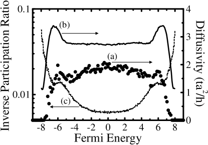
FIG. 3.: The result of the same computation of $\langle D_{x}(E_{F})\rangle$ as in Fig. 2, but for a different type of disorder, diagonal one of the strength $W=10$, introduced in the sample (the same labels apply to both figures).

The mesoscopic Kubo formula can be evaluated at any (continuous) Fermi energy. At first sight, it seems like that these leads to a much greater computational complexity than in the case of KFESR because of the need to find inverse matrix in Eq. (20) at each chosen energy, and then perform the trace over the site states ${\rm Tr}(\ldots)=\sum_{\bf m}\langle{\bf m}|(\ldots)|{\bf m}\rangle$. Namely, in the KFESR one needs to diagonalize Hamiltonian only once and then use obtained eigestates to compute matrix elements of velocity operator in the eigenbasis. However, this is only an apparent difficulty once the conservation of current is invoked. Since all Kubo formulas for conductance stem from Eq. (4), one has to assume (or choose) some electric field factors therein. Current conservation, i.e., the fact that $I$ has to be the same on each cross section, means that conductance is independent of this choice. The minimal space for tracing, when system is described by tight-binding Hamiltonian (TBH) in Eq. (21), is obtained by taking both factors ${\bf E}({\bf r})$ and ${\bf E}({\bf r}^{\prime})$ to be nonzero only on two adjacent planes of the lattice. Namely, the expectation value of the velocity operator (11) in the site representation is nonzero only between the states residing on adjacent planes,

$$\langle{\bf m}|\hat{v}_{x}|{\bf n}\rangle=\frac{i}{\hbar}t_{\bf mn}\left(m_{x}-n_{x}\right),$$ (27)

for a TBH (21) with nearest-neighbor hopping. The final result is then to be divided by $a^{2}$ [instead of $L_{x}^{2}$ in Eq. (19)].

Thus, only a block matrix $2N_{z}N_{y}\times 2N_{z}N_{y}$ of the Green function for the whole sample has to be computed explicitly (e.g., those elements which connect first two planes of the sample in Fig. 1). Because $[E-\hat{H}-\hat{\Sigma}^{r}]$ is a band-diagonal matrix of a bandwidth $2N_{y}N_{z}+1$, one can shorten the time needed to compute this block of the Green function (20) by finding the LU decomposition of a band-diagonal matrix, followed by forward-backward substitution for each needed Green function element. [50] This requires similar number of operations [51] as in the more familiar recursive Green function technique. [46]

III Transport through dirty metal junctions

This section studies the static DC transport properties of a metal junction composed of two disordered conductors with different kind of disorder introduced on each side of the contact interface. Both conductors are modeled as a disordered binary alloy (i.e., composed of two types of atoms, $A$ and $B$) using TBH of Eq. (21). The quenched disorder is simulated by taking the random on-site potential such that $\varepsilon_{\bf m}$ is either $\varepsilon_{A}$ or $\varepsilon_{B}$ with equal probability. Specifically, I take the lattice $18\times 8\times 10$ on each side of the junction and for the binary disorder: $\varepsilon_{A}=-4$, $\varepsilon_{B}=0$ on the left; and $\varepsilon_{A}=4$ and $\varepsilon_{B}=0$ on the right. Thus, the junction has naturally a rough interface [14] because of the random positions of three different types of atoms around the plane in the middle of the junction.

We commence with a description of the junction, as well as homogeneous samples used as a reference, in terms of traditional Kubo theory based on the KFESR (10). Although Ref. [46] stated as one of the motivations for undertaking the rigorous derivation of Landauer two-probe formula from KLRT, that traditional use of Kubo formula [25] was numerically demanding, today’s computers are much more powerful, and it is of interest to compare this method to a modern [16] mesoscopic use of the Kubo formula. Kubo theory permits the discussion of diffusivity $D_{\alpha}$ of an eigenstate $|\alpha\rangle$. This quantity is extracted directly from the KFESR for Fermi gas of noninteracting quasiparticles

$$\sigma=\frac{1}{\rho}=\frac{e^{2}}{\Omega}\sum_{\alpha}\left(-\frac{\partial f}{\partial E_{\alpha}}\right)D_{\alpha}=e^{2}N(E_{F})\bar{D}.$$ (28)

Thus, the quantum diffusivity is given explicitly by the following expression

$$D_{\alpha}^{x}=\pi\hbar\sum_{\alpha^{\prime}}|\langle\alpha|\hat{v}_{x}|\alpha^{\prime}\rangle|^{2}\delta(E_{\alpha}-E_{\alpha^{\prime}}).$$ (29)

In the semiclassical regime, $D_{\alpha}\rightarrow D_{k}=v_{k}\ell_{k}/3$. However, $D_{\alpha}$ can be used to characterize transport even in the nonperturbative regime where semiclassical concepts, like mean free path, loose their meaning. [21]

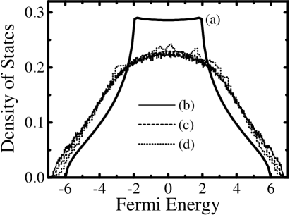
FIG. 4.: The density of states of: (a) clean metal ($W=0$); (b) dirty metal ($W=6$ on a lattice $15\times 15\times 15$ averaged over 50 disorder configurations), obtained as $N(E)=2/{\Omega}\,\sum_{\alpha}\delta(E-E_{\alpha})$ from the exact eigenspectrum $E_{\alpha}$ of a closed sample Hamiltonian; (c) dirty metal [$W=6$ on a lattice $10\times 10\times 10$ averaged over 50 disorder configurations], obtained from the imaginary part Eq. (32) of the Green function (20) of an open sample; (d) is computed in the same way as (c) except that smaller lattice $4\times 4\times 4$ is used.

To simplify calculations, I compute the quantum diffusivity $\langle D_{x}(E_{F})\rangle$ averaged over the disorder ($\langle\ldots\rangle$ denotes averaging over an impurity ensemble), as well as over a small energy interval. This is an additional transport information, obviously related to conductivity (28), which is not usually seen in the literature on disordered electron physics. [52] It has been exploited in the transport physics of glasses (e.g., to study the thermal conductivity in amorphous silicon [40]). The width $\eta$ of the Lorentzian $\bar{\delta}(E_{\alpha}-E_{\alpha^{\prime}})$ in (29) is chosen as some multiple of the local average level spacing $\Delta(E_{\alpha})$ in a small energy interval around the eigenenergy $E_{\alpha}$. The method of computing $\langle D_{x}(E_{F})\rangle$ is as follows: a set of eigenstates (the number of eigenstates is equal to the number of lattice sites $N_{s}=N\times N_{y}\times N_{z}$) is obtained by numerical diagonalization; $\mapsto$ for each eigenstate I compute $D_{\alpha}^{x}$, where summation is going over all states $|\alpha^{\prime}\rangle$ “picked” by the Lorentzian $\bar{\delta}(E_{\alpha}-E_{\alpha}^{\prime})$ (centered on $E_{\alpha}$) in an energy interval of $3\eta$ around $E_{\alpha}$; $\mapsto$ finally, I average the diffusivities over the disorder and energy interval defined by the bin of the size $\Delta E=0.0225$.

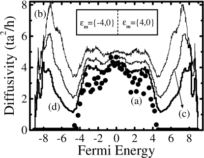
FIG. 5.: Diffusivity $\langle D_{x}(E_{F})\rangle$ for a metal junction composed of two disordered binary alloys (modeled by TBH on a lattice $36\times 8\times 10$): (a) computed using the Kubo formula (19) in terms of the Green function for the sample with attached leads; computed from the Kubo formula in exact single particle eigenstate representation (29), where the width of the Lorentzian broadened delta function is (b) $\eta=25\Delta(E_{F})$, (c) $\eta=10\Delta(E_{F})$, and (d) $\eta=5\Delta(E_{F})$. Disorder averaging is performed over 50 different samples.

The efficient way of calculating quantum-mechanical average values of some operator, like $\langle\alpha|\hat{v}_{x}|\alpha^{\prime}\rangle$ appearing in the definition of eigenstate diffusivity (29), is to multiply three matrices $\hat{\alpha}^{\dagger}\cdot\hat{v}_{x}\cdot\hat{\alpha}$, where $\hat{\alpha}$ is a matrix containing eigenvectors $|\alpha\rangle$ as columns, and then take modulus squared of each matrix element in such product. The number of operations in the naïve calculation of the expectation values of operator, where each of them is calculated separately, scales as $\sim N_{s}^{4}$, while in the method presented above it scales as $\sim N_{s}^{3}$ ($N_{s}\times N_{s}$ is the dimension of operator matrix). This procedure becomes a natural choice once we understand that it actually transforms the matrix of the operator $\hat{v}_{x}$ from the defining (site) representation into the representation of eigenstates $|\alpha\rangle$. The end result of the calculation, the average diffusivity $\langle D_{x}\rangle$, is related to the conductivity through Einstein relation

$$\sigma_{xx}=e^{2}N(E_{F})\langle D_{x}(E_{F})\rangle.$$ (30)

Here $N(E_{F})$ is the density of states (for both spin components) evaluated at the Fermi level $E_{F}$.

I first calculate $\langle D_{x}(E_{F})\rangle$ for the homogeneously disordered sample (with binary disorder $\varepsilon_{A}=-2$, $\varepsilon_{B}=2$) modeled on a lattice $18\times 8\times 10$, as shown in Fig. 2. To get an insight into the microscopic features of the eigenstates used to evaluate the KFESR (a few eigenstates around each $E_{F}$ determines the transport properties at $E_{F}$), this figure also plots the inverse participation ratio (IPR) [53]

$$I_{2}=\Delta\left\langle\sum_{{\bf m},\alpha}\,|\Psi_{\alpha}({\bf m})|^{4}\delta(E-E_{\alpha})\right\rangle,$$ (31)

averaged over disorder and energy $[\Psi_{\alpha}({\bf m})=\langle{\bf m}|\alpha\rangle]$. This is the simplest single-number measure of the degree of localization (i.e., the bigger the IPR the more localized is the state is, e.g. IPR$=N_{s}$ corresponds to a completely localized states on one lattice site). The IPR can also be related to the average return probability [19] that particle, initially launched in a state $|{\bf m}\rangle$ localized on a lattice site ${\bf m}$, will return to the same site after a very long time (which is determined by its diffusive properties encoded in $D_{\alpha}$). The second calculation, shown in Fig. 3, is for the homogeneous sample described by the standard Anderson model where $\varepsilon_{{\bf m}}\in[-W/2,W/2]$ is a uniform random variable. This results are to be compared to the reference calculation based on the mesoscopic Kubo formula.

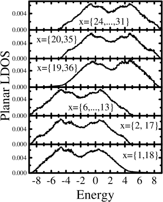
FIG. 6.: Local density of states (LDOS) integrated over the $y$ and $z$ coordinates inside the metal junction studied in Fig. 5. This “planar LDOS” $\rho(m_{x},E)$ is computed from the exact eigenstates of the TBH using Eq. (33). The result is plotted after $\rho(m_{x},E)$ is averaged over several planes along the $x$-axis (the planes used in this procedure are given on each panel).

Strictly speaking, the concept of eigenstate does not exist in open systems. Such systems can be characterized by non-Hermitian Hamiltonians, [18] which do not conserve total probability (cf. Sec. II). This is a consequence of a simple physical fact that an electron stays finite time within the sample before escaping into the surrounding leads (i.e., initial discrete energy levels are broadened by the coupling to the leads). Nonetheless, we can still get [22] the density of states (DOS) from the imaginary part of the Green function (20)

$$N(E_{F})=\sum_{{\bf m}}-\frac{1}{\pi}{\rm Im}\,\hat{G}^{r}({\bf m},{\bf m};E_{F}).$$ (32)

That such DOS of an open 3D system is indistinguishable from the one computed from the distribution of energy eigenvalues, $N(E_{F})=(2/\Omega)\,\langle\sum_{\alpha}\delta(E_{F}-E_{\alpha})\rangle$, is shown in Fig. 4. This is in spite of the fact that leads strongly perturb the edges of the system, which is clearly exhibited only on the smallest lattice in Fig. 4. Thus, the average diffusivity $\langle D_{x}(E_{F})\rangle$ can be computed in a straightforward manner from the Einstein relation (30) where conductivity is formally expressed from the disorder-averaged conductance $\sigma_{xx}=\langle G_{xx}\rangle L_{x}/S$ given by the mesoscopic Kubo formula.

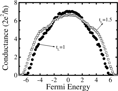
FIG. 7.: Two-probe conductance of a disordered conductor (averaged over 50 samples) modeled by the Anderson model with diagonal disorder $W=6$ on a simple cubic lattice $10^{3}$. The computation is done using the mesoscopic Kubo formula (19) for the finite sample attached to two semi-infinite leads characterized by two different values of hopping integral $t_{\rm L}$. Note that the conductance vanishes at $|E|=6t$ (band edge in a clean sample) when $t_{\rm L}=t$.

In both calculations for the homogeneous samples it appears that discrepancy between the Kubo formula in single particle representation (10) and the exact method, based on the formula (19) for the sample + lead system, is only numerical. In fact, the difference is very small in the disordered binary alloy and a bit larger in the Anderson model with continuous disorder. It originates from the ambiguity in using the width $\eta$ of the broadened delta function. Namely, nonzero $\eta$ effectively introduces inelastic scattering as an uncorrelated random event.[43] The increase of the diffusivity close to the band edges of diagonally disordered Anderson model (cf. Fig. 3) was seen long time ago in the direct simulations of the wave function diffusion performed in early days of localization theory. [52]

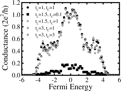
FIG. 8.: Two-probe conductance (averaged over 50 samples) of the same dirty metallic junction sample as in Fig. 5, but attached to two semi-infinite ideal leads with several different hopping integral $t_{\rm L}$ or lead-sample couplings $t_{\rm C}$ (hopping integral in the sample sets the unit of energy $t=1$). The computation is based on the mesoscopic Kubo formula Eq. (19).

The same analysis is repeated for a junction (introduced at the beginning of this section) which is composed of two different disordered binary alloys on each side. The result is shown in Fig. 5. Large fluctuations of the diffusivity (i.e., quantum conductance $G$ from which diffusivity is computed at specific $E_{F}$) are caused by the conductance being of the order of $2e^{2}/h$ (Fig. 8). Such fluctuations are less obvious in the result based on the KFESR because of the extra averaging over energy provided by the Lorentzian broadened delta function. Here the discrepancy between the two different methods is not only quantitative, but the KFESR (10) shows nonzero diffusivity (and thereby conductivity, since global DOS is nonzero all throughout the band) at Fermi energies at which there are no states on one side of the junction which can carry the current. [54] The result persist even when the width $\eta$ of the Lorentzian broadened delta function is decreased. Therefore, it is not an artifact of the numerical trick used to evaluate KFESR. The states which have nonzero amplitude all throughout the junction cease to exist at $|E_{b}|\sim 4.7$, which is seen by inspecting the local density of states (LDOS), integrated over $y$ and $z$ coordinates

$$\rho(m_{x},E) = \sum_{m_{y},m_{z}}\rho({\bf m},E)=$$ (33)

$$= \sum_{m_{y},m_{z}}\!\sum_{\alpha}\,|\Psi_{\alpha}({\bf m})|^{2}\,{\delta}(E-E_{\alpha}).$$ (34)

Such “planar LDOS” along the $x$-axis is plotted in Fig. 6. It changes abruptly while going from one side of the junction to the other side (except for the small tails near the interface). On the other hand, Fig. 5 explicitly demonstrates that Kubo formula (19) for an open finite-size sample plugged between ideal semi-infinite leads correctly describes this junction. Namely, the diffusivity vanishes at the same point at which LDOS goes to zero. It should be emphasized that once the leads are attached, two new interfaces (lead-sample) in the problem arise. The Landauer-Büttiker scattering approach to transport intrinsically takes care of these boundaries by considering the realistic finite-size system where electrons can leave or enter through some surfaces into the rest of the circuit represented by the leads. [45, 55] Thus, mesoscopic developments have clarified the way of proper application of Kubo formulism to finite-size samples (which is ultimately related to the eternal puzzle of the origins of dissipation in conservative systems, technically the only ones appearing in the Kubo analysis). [56] This in turn has justified heuristic arguments of Landauer on a rigorous basis. [46, 27]

The conductance of an infinite (sample + leads) system will go to zero at the band edge of a clean lead $|E_{b}|=6t$ if we use the same hopping parameter in the lead $t_{\rm L}=t$ as in the disordered sample. This stems from the fact that are no states in the leads which can carry the current for Fermi energies $|E_{F}|>6t$ outside of the clean TBH band. Technically, the self energy $\hat{\Sigma}^{r}$ is real at these energies, which leads to ${\rm Im}\,\hat{G}$ in (19) being zero. Thus, the conductance of the whole band of disordered sample cannot be computed unless we increase $t_{\rm L}$ in the leads. This is illustrated in Fig. 7 for the homogeneous sample described by the Anderson model where band edge of the disordered sample $|E_{b}|>6t$ lies outside of the clean metal band defined by crystal symmetry. Thus, a natural question arises when using $t_{\rm L},\,t_{\rm C}\neq t$: how sensitive is the conductance to the properties of leads or the sample-lead coupling? This problem resembles the quantum measurement problem because semi-infinite leads can also be viewed as a macroscopic apparatus necessary for measurement. [28, 58] This is further stressed in multi-probe geometries [18] where extra leads are introduced to measure the voltages along the sample (besides the two leads, used here, through which the current is fed). The measured conductance is then property of both the sample and the measurement geometry, which is one of the reasons for mesoscopic physics to employ only sample- and measurement geometry-specific quantities, like quantum conductance, instead of intensive quantity like conductivity. [36] From a transport point of view, it is clear that lead-sample interfaces introduce extra scattering for different effective masses or Fermi velocities in the sample and the lead. Thus, the exactness of the conductance calculated here is, in fact, a feature of the whole sample + leads setup in Fig. 1 (that is akin to any kind of measurement in quantum mechanics), and it is important to confirm that general conclusions about the relationship between different Kubo formulas do not depend on particular values of the chose parameters for the leads.

It is understood [57] that if broadening of the energy levels due to the coupling to semi-infinite leads is greater than the Thouless energy $E_{\rm Th}\simeq\hbar{\mathcal{D}}/L^{2}$, (${\mathcal{D}}=v_{F}\ell/3$ is the classical diffusion constant), then level discreteness of an isolated sample is unimportant and $G$ will be independent of the properties of leads. This limit corresponds to an “intrinsic” (Thouless) conductance $G/G_{Q}=2\pi E_{\rm Th}/\Delta$ ($\Delta$ is the mean level spacing) that is smaller than the conductance determined by the lead-sample contact. [59] It requires disordered enough sample [58] and leads of the same cross section as that of the sample. [59] Thus, even though attaching the sample to the leads brings dramatic changes (discrete spectrum is changed into continuous and new boundary conditions are introduced), the conductance is determined by the sample properties only, and dissipation in the reservoirs does not enter into computational algorithm. This dependence is studied in Fig. 8 by looking at the conductance of our model junction as a function of the hopping in the leads $t_{\rm L}$ and the coupling $t_{\rm C}$. The conductance is virtually independent of $t_{\rm L}$, which is a consequence of the smallness of the disordered junction conductance (as discussed above). It goes down drastically with decreasing of the coupling $t_{\rm C}$ (the same behavior is anticipated when $t_{\rm L}$ is increased substantially because of the increased reflection at the lead-sample interface).

IV Transport through strongly disordered interface

In this section we analyze quantum transport properties of a single dirty interface whose dimensionless conductance $G/G_{Q}$ is much smaller than the number of conducting channels $N_{\rm ch}$ (i.e., much smaller than the conductance of a ballistic conductor of the same cross section). For practical purposes, interface can be defined as a any scattering region whose thickness is sufficiently shorter than [5] $\lambda_{F}$ (in bulk conductors $L\gg\lambda_{F}$). Here we look at a geometrical plane of atoms as a model of interface in the strict sense. Furthermore, the evolution of transport from single dirty interface to strongly disordered thin slab (i.e., “thin Anderson insulators”, since stacking together enough finite-size interfaces, with the disorder strength chose here, would lead to a bulk Anderson insulator having exponentially small conductance). Such thin slabs are a more likely element in experimental circuits. [20] These problems are not only conceptual, namely to understand the difference between the transport in bulk conductors and interfaces, but it has been brought about by the understanding of crucial effects the interface scattering can have in the CPP transport experiments [60] on GMR magnetic multilayers (in GMR the added complication is spin-dependent interface resistance [61] which dominates the resistance and magnetoresistance for not too large layer thicknesses [62]).

The importance of interface scattering in many areas of metal and semiconductor physics has been realized in a plethora of research papers since the seminal work of Fuchs. [7] They are mainly concerned with the transport parallel to impenetrable rough interface, while recent have also risen interest in the transport normal to the interface (CPP geometry). Because the nature of the transport relaxation time in inhomogeneous systems is not well understood, [4] the first step is to understand properties of a single interface before studying them as a part of some more complicated circuit like those in Sec. V. For example, the properties of a single interface cannot be described in terms of the Boltzmann conductivity $\sigma_{B}=ne^{2}\tau/m$, i.e., using the elastic mean free path $\ell=v_{F}\tau$ (or transport mean free time $\tau$) familiar from the bulk metallic conductors whose conductivity is dominated by the semiclassical effects.

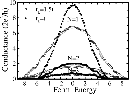
FIG. 9.: Conductance of a single dirty interface ($N=1$) and thin slabs composed of two ($N=2$) or three ($N=3$) such interfaces (modeled by the Anderson model with diagonal disorder $W_{I}=30$ on a lattice $N\times 10\times 10$). The calculation is performed using different values of the hopping parameter $t_{\rm L}$ in the attached leads, and the results are averaged over $200$ realizations of disorder.

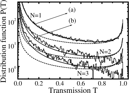
FIG. 10.: Distribution function $P(T)$ of the transmission eigenvalues (at half-filling $E_{F}=0$) for a single disordered interface $N=1$, and thin slabs composed of two $N=2$ or three $N=3$ such interfaces, modeled by the Anderson model with $W_{I}=30$ on a cubic lattice $N\times N_{y}\times N_{z}$. The disorder-average is taken over an ensemble of $1000$ conductors. The analytical functions plotted are: (a) $P(T)=(G/2G_{Q})\,1/(T^{3/2}\sqrt{1-T})$, and (b) Dorokhov distribution $P(T)=(G/2G_{Q})\,1/(T\sqrt{1-T})$.

Lacking enough experimental information, the simple theoretical models for the interface effects on electron propagation assume diffuse scattering at interdiffused atoms or interfacial roughness [63] (these free electron theories omit the complex electronic band structure of transition metals appearing in realistic GMR samples). Even disorder-free interface can have a nonzero resistance, because of mismatch of the crystal potential and band structures. [4] Here we are interested only in generic properties of mesoscopic transport through interfaces that do not depend on material-specific details. [5] Therefore, the interface roughness is modeled here by the short range random scattering potential [12] generated by the impurities located on the sites of a square lattice $1\times N_{y}\times N_{z}$ and with strong disorder $W_{I}=30$ in the corresponding TBH Eq. (21). The bulk conductor composed of such interfaces (stacked in parallel and coupled with nearest neighbor hopping $t$) is an Anderson insulator, because all states are localized already for [64] $W_{c}\simeq 16.5$. To compute the CPP transport properties using the mesoscopic Kubo formula (19), the interface is placed in our standard computational setup between the two semi-infinite disorder-free leads. Thus, the conductance is computed for an atomic monolayer of a disordered material inside an infinite clean sample of a finite cross section shown in Fig. 1. Also computed is the conductance of a thin slab composed of two (i.e., 3D conductor modeled on the lattice $2\times N_{y}\times N_{z}$) and three sheets ($3\times N_{y}\times N_{z}$) of the same disordered material, as shown in Fig. 9. The microscopic origin of different terms contributing to the interface resistance was traced back to both specular and diffusive scattering in the plane (where diffusive scattering can even open additional channels for electron transport, thereby increasing the conductance). [4]

Following the discussion in Sec. III, the influence of the leads on the interface conductance is checked by using two different hopping integrals $t_{\rm L}$ (compare to Fig. 7). Here the analysis based on comparison of relevant energy scales does not work (i.e., one can not use bulk material concepts, like $E_{\rm Th}$). Plausibly, I find that leads affect the conductance of the interface much more than the conductance of a bulk disordered conductor (with similar value of disorder-averaged conductance).

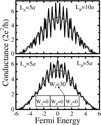
FIG. 11.: The disorder-averaged (over 200 configurations) conductance of a mesoscopic multilayer, composed of dirty interfaces and clean bulk conductors, modeled on a lattice $17\times 10\times 10$. The results are obtained from: the mesoscopic Kubo formula (19) applied to the whole multilayer (solid line); and using the semiclassical resistor model, $G_{\rm RM}=(2R_{I}-R_{\rm QPC})^{-1}$ (dotted line), where individual resistances are computed also from Eq. (19) and summed accordingly (the meaning of $R_{\rm QPC}$ is explained in Fig. 15).

Mesoscopic transport methods give the possibility not only to compute the conductance, but also to use the picture of conducting channels and their quantum-mechanical transmission properties. From a pragmatical point of view, one does not need these fully quantum techniques to study the transport in macroscopic conductors which are usually dominated by semiclassical physics. Nevertheless, the study of the distribution of transmission probabilities, which requires phase-coherent transport, enhances our insight into the conduction processes in electronic systems. The diagonalization of a Hermitian matrix ${\bf t}{\bf t}^{\dagger}$, which defines the conductance through the Landauer formula,

$$G = \frac{2e^{2}}{h}\,\text{Tr}\,({\bf tt}^{{\dagger}})=\frac{2e^{2}}{h}\sum_{n=1}^{N_{y}N_{z}}T_{n},$$ (36)

$${\bf t} = 2\sqrt{-\text{Im}\,\hat{\Sigma}_{L}}\,\hat{G}^{r}_{1N}\sqrt{-\text{Im}\,\hat{\Sigma}_{R}},$$ (37)

introduces a set of transmission eigenvalues $0\leq T_{n}\leq 1$

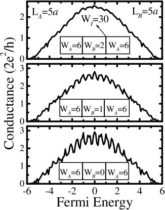
FIG. 12.: The disorder-averaged (over 200 configurations) conductance of a mesoscopic multilayer, composed of strongly disordered interfaces and (quasi)ballistic bulk conductors (e.g., $\ell\approx 9$ at half-filling for $W=2$), modeled on a lattice $17\times 10\times 10$. The results are obtained from the mesoscopic Kubo formula (19) applied to the whole multilayer as a single quantum-coherent conductor.

for each realization of disorder. The incident flux concentrated in channel $|p\rangle$ will give the wave function in the opposite lead $\sum_{q}{\bf t}_{pq}|q\rangle$, where ${\bf t}$ is the transmission matrix. Here $\hat{G}^{r}_{1N}$ is the matrix block, which connects layers $1$ and $N$ of the sample, of the full retarded real-space Green function matrix (20). The distribution function of $T_{n}$ is defined as

$$P(T)=\left\langle\sum_{n}\delta(T-T_{n})\right\rangle.$$ (38)

Using $P(T)$, the disorder-average value of any quantity that can be written down in the form of linear statistics $a(T)$ can be expressed as [65]

$$\langle A\rangle=\left\langle\sum_{n=1}^{N_{\rm ch}}a(T_{n})\right\rangle=\int\limits_{0}^{1}dT\,a(T)P(T).$$ (39)

For example, the conductance is described by a linear statistics $g(T)=T$. Contrary to the naïve expectations, stemming from comparison with Drude-Boltzmann conductance $G\simeq G_{Q}N_{\rm ch}\ell/L$, that transmission of every channel is $T\simeq\ell/L$ in the metallic diffusive ($G_{Q}N_{\rm ch}\gg G\gg G_{Q}$) bulk conductor, it was shown by Dorokhov [66] that in a homogeneous multichannel wire geometry

$$P_{\rm D}(T)=\frac{G}{2G_{Q}}\,\frac{1}{T\sqrt{1-T}},\\ \ \cosh^{-2}\left(\frac{N_{\rm ch}}{g}\right)<T<1.$$ (40)

The cutoff [5] at small $T$ is such that $\int_{0}^{1}dT\,P(T)=N_{\rm ch}$ ensuring that averages of the first and higher order moments of $T$ are not affected (on the proviso $N_{\rm ch}\gg G/G_{Q}$). The Dorokhov distribution is universal—it depends only on the disorder-averaged conductance $G$ and not on the details of disorder, dimension, shape of the sample, carrier density, spatial resistivity distribution and other sample-specific properties. [65] Thus, $P(T)$ is bimodal distribution function meaning that: most of $T_{n}$ are either $T_{n}\simeq 0$ (“closed” channels) or $T_{n}\simeq 1$ (“open” channels). This has important consequences when calculating linear statistics other than the conductance since we can get conductance (first moment of the distribution) without really knowing the details of $P(T)$ (e.g., the higher moments are probed in the case [65] of shot-noise power, Andreev conductance of metal/supercondcutor interface, etc.).

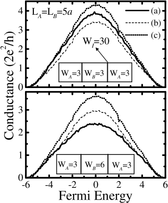
FIG. 13.: The disorder-averaged (over 200 configurations) conductance of a mesoscopic multilayer, composed of strongly disordered interfaces and weakly disordered bulk conductors, modeled on a lattice $17\times 10\times 10$ ($\ell\approx 4a$ at half-filling for $W=3$). The results are obtained from: (a) mesoscopic Kubo formula (19) evaluated for the whole multilayer; following the resistor model Eq. (43), (b) $G_{\rm RM}^{\prime}=(2R_{A}+R_{B}+2R_{I})^{-1}$, and (c) $G_{\rm RM}=(2R_{A}+R_{B}+2R_{I}-4R_{\rm QPC})^{-1}$.

The simple counting of the number of $T_{n}$ in each bin along the interval $[0,1]$ gives allows us to obtain the distribution function $P(T)$ (in this procedure the delta function in (38) is effectively broadened into a box function $\bar{\delta}(x)$ equal to one inside each bin). Figure 10 plots $P(T)$ for the dirty interface and the two thin slabs. The result is compared to $P_{\rm D}(T)$ of Eq. (40) and the one which describes the numerical data

$$P_{\rm fit}(T)=\frac{G}{2G_{Q}}\,\frac{1}{T^{3/2}\sqrt{1-T}}.$$ (41)

This formula is, up to a numerical factor, the same as the analytical prediction of Schep and Bauer [5] for a single dirty interface

$$P_{\rm SB}(T)=\frac{G}{\pi G_{Q}}\,\frac{1}{T^{3/2}\sqrt{1-T}},$$ (42)

Thus, interfaces belong to a universality class different from that of diffusive bulk conductors characterized by the Dorokhov distribution $P_{\rm D}(T)$. However, it seems that distribution is valid even for thin slabs whose thickness $L$ is grater than $\lambda_{F}$, but is smaller than the localization radius (which in our case can be estimated in the pedestrian way as the thickness at which conductance vanishes). This is in compliance with experimental confirmation of $P_{\rm SB}(T)$ in a uniform Nb/AlO_x/Nb Josephson junction, whose subharmonic gap structure in the $I-V$ characteristic is extremely sensitive to the number of conducting channels at $E_{F}$ and their transmission probabilities [67], since the thickness of the realistic AlO_x barrier is bigger than $\lambda_{F}$ in the junction electrodes (Ref. [20] gives a simple derivation of the Schep-Bauer distribution without using the assumption $L\ll\lambda_{F}$). In fact, even our extremely high disorder input in the standard Anderson model generates surface conductance in the band center, $g_{I}\simeq 9\cdot 10^{10}\ \Omega^{-1}$cm^-2 (for $a=3$ Å), that is much higher than $10^{8}\,\Omega^{-1}$cm^-2 reported for the measured value in Ref. [20] (suggesting that thin slab is more likely to play to role of a barrier in these Josephson junction than the strict geometrical plane). While being intriguing concept in disorder electron physics, universality can be frustrating for the device engineers. Not all features of the transport through dirty interface are universal. [5]

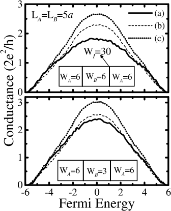
FIG. 14.: The disorder-averaged (over 200 configurations) conductance of a mesoscopic multilayer, composed of strongly disordered interfaces and weakly disordered bulk conductors, modeled on a lattice $17\times 10\times 10$. The results are obtained from: (a) mesoscopic Kubo formula (19) evaluated for the whole multilayer; following the resistor model Eq. (43), (b) $G_{\rm RM}^{\prime}=(2R_{A}+R_{B}+2R_{I})^{-1}$, and (c) $G_{\rm RM}=(2R_{A}+R_{B}+2R_{I}-4R_{\rm QPC})^{-1}$.

V Transport through multilayers

Armed with the knowledge of transport properties of dirty interfaces and metallic homogeneous layers, we can now undertake the study of circuits composed of such elements. The main feature of our circuits is that they are of nanoscale size ($\sim$ few $\lambda_{F}$) and fully phase-coherent (i.e., effectively at zero temperature). The choice of disorder and size of the system is driven by the interest here to explore the patterns of breaking (under the influence of quantum effects) of a simple description of the multilayer in terms of classical resistor network. Therefore, I study such deviations from semiclassics by computing the exact zero-temperature conductance of several multilayers, as well as of their components, using mesoscopic Kubo formula (19). This computation takes into account all quantum interference and quantum size effects from the onset. In general, resistors can be added according to the classical Ohm’s law only when their size is larger than the dephasing length $L_{\phi}$ (in this case the quantum features of diffusion can still enter through the transport properties of individual phase-coherent units of size $L_{\phi}$, example being the weak localization effect [44] at finite temperatures). For example, at high enough temperatures the system can be partitioned into the cubes of a macroscopic size $L_{\phi}$ where quantum interference between wave functions scattered in different cubes can be neglected—this makes it possible then to define an intensive quantity, [22] like conductivity, by solving a classical random resistor network problems. [69] The quantum composition law for quantum resistors in a chain is more complicated since it contains a phase variable depending on the characteristics of all scatterers. [70, 71] Thus, because of quantum interference effects (like conductance fluctuations [72]) phase-coherent resistors do not add in series, and even for homogeneous samples resistance as a function of length is not a self-averaging quantity (therefore requiring disorder-averaging to restore the Ohmic scaling [21, 73]). In the Landauer-Bẗtiker scattering formalism, resistor network description corresponds to a semiclassical concatenation of the scattering matrices of individual units (${\bf t}$ in (11) is just one block of a full scattering matrix [65]), i.e., the concatenation of “probability scattering matrices” of successive disordered regions (obtained by replacing each element of the scattering matrix by its squared modulus [68]).

The multilayers studied here are composed of three bulk conductors joined through two dirty interfaces. The whole structure is modeled by the TBH Eq. (21) on a lattice $17\times 10\times 10$ where sixth and twelfth monoatomic layers contain the same interface studied in Sec. IV. The disorder strength within the plane of the interface is fixed to $W_{I}=30$, while disorder inside the bulk layers (composed of five monolayers) is varied. The disorder strength is taken to be the same in two outer layers where diffusive bulk scattering takes place. This type of multilayer can be viewed as a period of an infinite $A/B$ multilayer: [63] layer of material $A$ on the outside (of resistivity $\rho_{A}$ and total thickness $2L_{A}=10a$, where $a$ is the lattice spacing) and interlayer material $B$ between the interfaces (of resistivity $\rho_{B}$ and thickness $L_{B}=5a$). For example, for the chosen disorder strengths $W=3$ and $W=6$ the corresponding bulk material resistivities at half-filling are $\rho\simeq 130\,\mu\Omega$cm and $500\,\mu\Omega$cm (assuming $a=3{\text{\AA}}$), respectively. I neglect any potential step at the interface (caused by the conduction band shift at the interface [4]). Such multilayers are often described semiclassicaly in terms of the resistor model [24]

$$R_{\rm RM}=N_{b}\left(\rho_{A}\frac{2L_{A}}{S}+\rho_{B}\frac{L_{B}}{S}+2R_{I}\right),$$ (43)

where $R_{\rm RM}$ is the total multilayer resistance, $N_{b}$ is the number of bilayers (I study below just one multilayer period $N_{b}=1$), and $R_{I}$ is the interface resistance (evaluated in Sec. IV in Fig. 9). Thus, the resistor model treats both bulk and interface resistances as semiclassical elements of a circuit in which resistors add Ohmically in a series. Nevertheless, quantum diffusion can be important inside each individual resistor element, as discussed above. [18] From the measurement of $R_{\rm RM}$ as a function of the layer thickness, the bulk and interface resistances can be extracted experimentally. When quantum interference effects become important in the CPP transport, this picture breaks down.

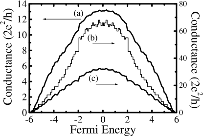
FIG. 15.: Conductance of individual resistors comprising the multilayers of Sec. V: disordered conductors modeled by the Anderson model a lattice $5\times 10\times 10$ with diagonal disorder strength, (a) $W=6$, and (b) $W=3$, and quantum point contact conductance ($1/R_{\rm QPC}$) of a clean sample modeled on the lattice with the same cross section (i.e., on a lattice supporting $100$ conducting channels, where the maximum of open channels with $T_{n}=1$ at the Fermi level in such 3D ballistic conductors [58] is $68$ at $|E_{F}|\simeq 0.3$).

The quantum (i.e., zero-temperature) conductance of the multilayers is computed using a standard tool throughout the paper—mesoscopic Kubo formula of Eq. (19) where whole multilayer is treated as a single phase-coherent unit. This approach intrinsically takes into account finite-size effects in the problem, [45] as emphasized in Sec. II, as well as all single-particle quantum interference effects. In all calculations the hopping integrals throughout the disordered sample and in the leads are the same ($t_{\rm L}=t_{\rm C}=t$). This means that no additional scattering, discussed in Sec. III), is generated at the lead-sample interface. [58] The remaining resistance can sometimes be interpreted as a series addition of two quantum resistors. Namely, the semiclassical limit of the two-probe Landauer or Kubo formula for conductance, obtained e.g., from the stationary-phase approximation [74] of the Green function expression (11) for the transmission of the sample, leads to

$$\langle G\rangle^{-1}=R_{\rm QPC}+\rho\frac{L}{S},$$ (44)

which should be valid for not too strong scattering on impurities. The “contact” resistance [75] $R_{\rm QPC}=\pi\hbar/e^{2}N_{\rm ch}$ is nonzero even for ballistic conductor because a finite cross section can carry only finite currents (the voltage drop in this case occurs at the lead-reservoir interface). Similar interpretation was given for the interface resistance, [63] and is expected to be valid also for the interfaces embedded into a multilayer if there is no coherent scattering between adjacent interfaces (e.g., when such effects are destroyed by sufficiently strong scattering in the bulk). These formulas naturally lead to the resistor model where different interfaces and bulk layers contribute to the CPP resistance as resistors in series. It is often assumed that $R_{\rm QPC}$ can be neglected when compared to usually much higher resistance of a diffusive sample, thus making the choice of the two-probe (or some other) geometry just the matter of computational convenience. [59]

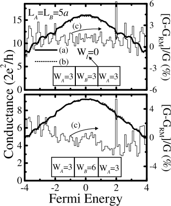
FIG. 16.: The disorder-averaged (over 200 configurations) conductance of a mesoscopic multilayer, composed of strongly disordered interfaces and weakly disordered bulk conductors, modeled on a lattice $17\times 10\times 10$. The results are obtained from: (a) mesoscopic Kubo formula (19) evaluated for the whole multilayer; and (b) following the resistor model Eq. (43), $G_{\rm RM}=(2R_{A}+R_{B}-2R_{\rm QPC})^{-1}$. The relative error $[G-G_{\rm RM}]/G$ is plotted as (c).

Since resistor model is expected to be retrieved in the limit of completely diffusive scattering in the bulk and lack of phase coherence, [63, 76] in the quest for substantial quantum effects induced deviations from this picture I start from the opposite limit: a multilayer composed of clean (ballistic) layers and disorder introduced on the interfaces, $W_{A}=W_{B}=0$ and $W_{I}=30$. The disorder-averaged result is plotted in Fig. 11 for two different thicknesses of the interlayer. Even after disorder-averaging, the conductance oscillates as a function of $E_{F}$. This clearly quantum effect is a consequence of the size quantization caused by a coherent interference of electrons reflected back and fort at the strongly disordered interface. After adding the disorder into the outer layers, the effect persists albeit with a smaller amplitude of oscillations (Fig. 12). However, while this is plausible because of the interlayer being composed of only few atomic monolayers [4] (i.e., its length is of the order of $\lambda_{F}$), it is somewhat surprising that oscillations increase with increasing the separation between the interfaces. Furthermore, the oscillating conductance is still quite different from a pure resonant tunneling conductance peaks which would occur at the energies of bound states if interfaces are replaced by the tunneling barriers [18] (e.g., in our model this can be generated by reducing the hopping integral $t_{\bf mn}$ between the outer layers and the interlayer [58]). Although it is obvious that this phenomenon cannot be accounted by the semiclassical resistor model, its answer is plotted for the sake of comparison. Also, by adding impurities in the interlayer we can follow the disappearance of conductance oscillations (which is akin to the studies of disorder effects on conductance quantization in ballistic conductors [48]). The effect has almost vanished at $W=2$ although the mean free path, e.g., around the band center, $\ell\approx 9$ (obtained from Bloch-Boltzmann equation with Born approximation for the scattering on a single impurity [21]) is still larger than $L$ (i.e., the transport within interlayer has not yet reached the limit of fully diffusive bulk scattering).

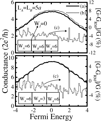
FIG. 17.: The same calculation as in Fig. 16 (the same labels apply), but for a slightly different multilayer with increased disorder strength in the two outer layers.

To sweep through the transition between fully quantum and (expected) resistor model semiclassical description, a disorder is introduced in both layers $A$ and $B$. The results are shown in Figs. 13 and 14. The disorder $W=6$ is the strongest one in the Anderson model where one can still use the semiclassical picture of transport at half-filling (i.e., at $E_{F}=0$ we get [21] $\ell\sim a$ for $W\simeq 6$, but localization is postponed to much higher values of [64] $W\simeq 16.5$). The other type of homogenous layer is modeled with $W=3$, which is in the crossover between the ballistic and the diffusive transport regime, since $\ell\approx 4$ at $E_{F}=0$ and $L_{A}=L_{B}=5a$. The statistical error bars on the disorder-averaged conductance (over $N_{\rm conf}$ samples), defined as $\Delta G=\sqrt{{\rm Var}\,G/N}$, are smaller than the size of the dots (this further clarifies that small conductances of the multilayers are not the consequence of strong disorder, but are generated by combining few metallic resistors and dirty interfaces in a series). The conductances of individual layers are plotted in Fig. 15. In the first case $W_{A}=W_{B}=3$, the naïve application of the resistor model, where $R_{\rm QPC}$ is neglected, leads to $G_{\rm RM}^{\prime}$ ($G_{\rm RM}=1/R_{\rm RM}$ is the sum of component resistances) being smaller than the quantum $G$ computed for the multilayer as a single coherent unit. However, the subtraction of four $R_{\rm QPC}$, which brings $G_{\rm RM}$ into the form of Eq. (44), gives conductance higher than $G_{\rm RM}>G$. Here $R_{\rm QPC}$ is the resistance of a ballistic conductor (“quantum point contact”) with a cross section $A=100a^{2}$ (see Fig. 15). According to Eq. (44), the resistances of homogeneous layer components of the multilayer, which are plotted in Fig. 15 (or Fig. 9 for the interface alone), are the sum of their “intrinsic bulk” resistance [59] and $R_{\rm QPC}$. Thus, when adding these resistors the final sum should contain only one $R_{\rm QPC}$ if resistor model is to be compared with the two-probe resistance of the multilayer. In all other cases which include layer with diagonal disorder $W=6$, both naïve and more careful attempt (where $(N_{R}-1)$ contact resistances $R_{\rm QPC}$ are subtracted from the sum of resistance of component layers, where $N_{R}$ is the number of bulk and interface resistances used to obtain such sum) to use the resistor model give the conductances which are greater than the ones computed for the multilayer as a single conductor. The explanation which invokes only extra scattering on the boundaries between different components inside the multilayer, which does not work in the first case $W_{A}=W_{B}=3$, is not the only one possible.

It was shown recently [21] that even in weakly disordered metals (where Boltzmann resistivity is practically indistinguishable from the one computed from Kubo formula) clear separation of a two-probe resistance into contact term and diffusive bulk resistance, as implied by the standard arguments of Eq. (44), is tempered by localization effects [i.e., terms of the order $\ell/L$ which are neglected in Eq. (44)], and therefore possible only in very weakly disordered systems. To elucidate the effects responsible for the difference between the two ways of evaluating the multilayer conductance in Figs. 13 and 14, I apply the same analysis on a multilayer where dirty interfaces are removed (i.e., $\varepsilon_{\bf m}=0$ on the sixth and twelfth plane along the $x-$axis). When $W_{A}\neq W_{B}$ such multilayers are similar to the junction studied in Sec. III where interface is not explicitly modeled as in Sec. IV, but appears as a boundary between two different homogeneous materials brought into a contact. In the opposite case $W_{A}=W_{B}$, the sample akin to a homogeneously disordered conductor whose conductance was studied in Fig. 7. The results of this calculations, plotted in Figs. 16 and 17, hint that difference between resistor model conductance $G_{\rm RM}$ and conductance $G$ of the multilayer as one indivisible quantum-coherent unit is quite minuscule, on the proviso that extraneous contact resistance terms are properly subtracted. Even though the multilayers are mesoscopic, where electrons retaining their phase coherence and are subject thereby to quantum interference effects, disorder averaging effectively destroys most of random interference terms (a sample self-averages at finite temperatures when it can be partitioned into a cubes of size $L_{\phi}$, as discussed above). [77] The surviving interference terms are exemplified by those generated by quantum interference effects on special trajectories (i.e., Feynman paths), such as the closed loops responsible for weak localization. [78] These nonlocal weak localization effects, arising from the interference between the amplitudes along the conjugated time-reversed loops which span the whole phase-coherent sample, are responsible for $G$ being slightly smaller than $G_{\rm RM}$ (localization effects inside the individual resistors, summed in the resistor model formula, are taken into account even by the semiclassical approach). As expected in this picture, the discrepancy is very small at $W=3$, and is increasing for stronger disorder [21] $W=6$. On the other hand, conductance fluctuations sneak in through the fluctuations of relative error $[G-G_{\rm RM}]/G$ of the resistor model as a function of Fermi energy (cf. Figs. 16 and  17).

VI Conclusions

I have studied different macroscopically inhomogeneous mesoscopic disordered 3D conductors by employing both fully quantum description, provided by the mesoscopic two-probe Kubo, and semiclassical resistor model. Before embarking on the technicalities of computations some fundamental issues in the quantum transport theory have been scrutinized: the relationship between the Kubo formula in exact single-particle eigenstate representation and Kubo formula for the finite-size sample inspired by mesoscopic physics; the influence of the macroscopic leads (“measuring apparatus”) on the computed two-probe conductance; and the transmission and transport properties of a single dirty interface, which are markedly different from a standard notions developed for bulk conductors. It was shown, by exact computation on examples of homogenous disordered samples and inhomogeneous metal junctions, that mesoscopic Kubo formula allows one to obtain the reliable results for the static zero-temperature conductance (which includes the properties of the attached leads) characterizing noninteracting quasiparticle transport. On the other hand, the evaluation of the traditional Kubo formula, based on the exact diagonalization of the respective Hamiltonian, ends up with a numerical discrepancy when compared to mesoscopic methods applied to homogeneous samples (because of the necessity to handle small numerical parameters, like the width of Lorentz broadened delta function), but qualitative fails in the case of inhomogeneous samples. This can be traced back to the conceptual obstacles in applying methods derived for an infinite sample to a finite-size system (even after it is extended through periodic boundary conditions) where the problem of dissipation and effect of the sample boundaries (which is crucial for the description of mesoscopic devices) have been traditionally bypassed for the sake of computational pragmatism.

The study of a single dirty interface, with specific Anderson model type disorder, shows that its transmission properties are well-accounted by the Schep-Bauer distribution, but these formula applies approximately also to thin slabs composed of a few of such interfaces (which is important for experimental investigations where one hardly deals with geometrical planes of theoretical analysis). The nanoscale mesoscopic multilayers containing such interfaces and ballistic bulk conductors exhibit disorder-averaged oscillating conductance as a function of Fermi energy. This effect of phase-coherence and quantum size effect is slowly destroyed upon adding the disorder inside the layers. However, even for diffusive scattering in the metallic layer components, smooth disorder-averaged multilayer conductances can not be completely accounted by the resistor model (which sums layer and interface resistances as resistors connected in series). Since this classical approach works well when interfaces are removed (up to a tiny localization effects arising from interference effects inside the whole sample), we can conclude that just a single plane of a strongly disordered material is enough to bring new quantum effects into the conductance of mesoscopic metallic multilayered structures.

I am grateful to P. B. Allen for guidance and unlimited supply of intriguing questions, and to I. L. Aleiner and J. A. Vergés for valuable discussions. This work was supported in part by NSF grant no. DMR 9725037.

$*$ Present address: Department of Physics, Georgetown University, Washington, DC 20057-0995.

REFERENCES

- [1] M. N. Baibich, J. M. Broto, A. Fert, F. Nguyen Van Dau, F. Petroff, P. Etienne, G. Creuzet, A. Friedrich, and J. Chazelas, Phys. Rev. Lett. 61, 2472 (1988).
- [2] G. Binach, P. Grünberg, F. Saurenbach, and W. Zinn, Phys. Rev. B 39, 4828 (1989).
- [3] V. K. Dugaev, V. I. Litvinov, and P. P. Petrov, Phys. Rev. B 52, 5306 (1995).
- [4] M.A.M. Gijs and G.E.W. Bauer, Adv. Phys. 46, 286 (1997), and references therein.
- [5] K. M. Schep and G. E. W. Bauer, Phys. Rev. B 56, 15 860 (1997).
- [6] H. Y. Fan, Phys. Rev. 61, 365, (1942); 62, 388 (1942).
- [7] K. Fuchs, Proc. Philos. Camb. Soc. 34, 100 (1938).
- [8] E. H. Sondheimer, Adv. Phys. 1, 1 (1952).
- [9] X.-G. Zhang and W. H. Butler, Phys. Rev. B 51, 10 085 (1995).
- [10] Mesoscopic Quantum Physics, edited by E. Akkermans, J.-L. Pichard, and J. Zinn-Justin, Les Houches, Session LXI, 1994 (North-Holland, Amsterdam, 1995).
- [11] R. Landauer, IBM J. Res. Dev. 1, 223 (1957); Phil. Mag. 21, 863 (1970); M. Büttiker, Phys. Rev. Lett. 57, 1761 (1986).
- [12] G. E. W. Bauer, A. Brataas, K. Schep, and P. Kelly, J. Appl. Phys. 75, 10 (1994).
- [13] G.E.W. Bauer, Phys. Rev. Lett 69, 1676 (1992).
- [14] Y. Asano, A. Oguri, and S. Maekawa, Phys. Rev. B 48, 6192 (1993).
- [15] C. Caroli, R. Combescot, P. Nozieres, and D. Saint-James, J. Phys C 4, 916 (1971); Y. Meir and N. S. Wingreen, Phys. Rev. Lett. 68, 2512 (1992).
- [16] B.K. Nikolić, Phys. Rev. B 64, 165303 (2001).
- [17] S. Sanvito, C.J. Lambert, J.H. Jefferson, and A.M. Bratkovsky, Phys. Rev. B 59, 11 936 (1999).
- [18] S. Datta, Electronic Transport in Mesoscopic Systems (Cambridge University Press, Cambridge, 1995).
- [19] B. Kramer and A. MacKinnon, Rep. Prog. Phys. 56, 1469 (1993).
- [20] Y. Naveh, V. Patel, D.V. Averin, K.K. Likharev, and J.E. Lukens, Phys. Rev. Lett. 85, 5404 (2000).
- [21] B. K. Nikolić and P. B. Allen, Phys. Rev. B 63, R020201 (2001).
- [22] M. Janssen, Phys. Rep. 295, 1 (1998).
- [23] J. Rammer, Quantum Transport Theory (Perseus Books, Reading, 1998).
- [24] S. Zhang and P.M. Levy, J. Appl. Phys. 69, 4786 (1991).
- [25] J. Stein and U. Krey, Z. Phys. B 37, 13 (1980).
- [26] P.A. Lee and T.V. Ramakrishnan, Rev. Mod. Phys. 57, 287 (1985).
- [27] H. Baranger and A. D. Stone, Phys. Rev. B 40, 8169 (1989); J. U. Nöckel, A. D. Stone, and H. U. Baranger, Phys. Rev. B 48, 17 569 (1993).
- [28] K. B. Efetov, Supersymmetry in Disorder and Chaos (Cambridge University Press, Cambridge, 1997).
- [29] M. C. Payne, J. Phys.: Condens. Matter 1, 4931 (1989).
- [30] Yu. V. Nazarov, Phys. Rev. Lett. 73, 134 (1994).
- [31] C. L. Kane, R. A. Serota, and P. A. Lee, Phys. Rev. B 37, 6701 (1988).
- [32] Technical subtleties (like proper order of non-commuting limits) in finding zero and nonzero surface terms in the microscopic formulation of linear transport in open systems are accounted in Ref. [27].
- [33] C. L. Kane, P. A. Lee, and D. P. DiVincenzo, Phys. Rev. B 38, 2995 (1988).
- [34] For a long time it seemed that these rigorous (quantum) formulations of transport were merely serving to justify the intuitively appealing Boltzmann approach. The new viewpoint came with the first explicit calculation of quantum corrections like weak localization [44]—a quantum interference effect which generates a negative correction term to the Boltzmann result, and is responsible at low temperatures for all of the temperature and magnetic field dependence.
- [35] The relation of “vanishing” to the other relevant energy scales in the linear (quantum) transport regime is reviewed in Ref. [18].
- [36] A. D. Stone, in Ref. [10].
- [37] B. Nikolić and P. B. Allen, Phys. Rev. B 60, 3963 (1999).
- [38] E. Abrahams, P. W. Anderson, D. C. Licciardello, and T. V. Ramakrishnan, Phys. Rev. Lett. 42, 673 (1979).
- [39] R. Berkovits, J.W. Kantelhardt, Y. Avishai, S. Havlin, A. Bunde, cond-mat/0012075.
- [40] J. L. Feldman, M. D. Kluge, P. B. Allen, and F. Wooten, Phys. Rev. B 48, 12 589 (1993).
- [41] R. Kubo, S. I. Miyake, and N. Hashitsume, in Solid State Physics, edited by F. Seitz and D. Turnbull (Academic Press, New York, 1965), vol. 17, p. 288.
- [42] E. N. Economou Green’s Functions in Quantum Physics (2nd ed., Springer-Verlag, Berlin, 1990).
- [43] D. J. Thouless and S. Kirkpatrick, J. Phys. C 14, 235 (1981).
- [44] L. P. Gor’kov, A. I. Larkin, D. E. Khmel’nitskii, Pis’ma Zh. Eksp. Teor. Fiz. 30, 248 (1979) [JETP Lett. 30, 228 (1979)].
- [45] Y. Imry and R. Landauer, Rev. Mod. Phys. 71, S306 (1999).
- [46] D. S. Fisher and P. A. Lee, Phys. Rev. B 23, 6851 (1981).
- [47] X.-G. Zhang and W. H. Butler, Phys. Rev. B 55, 10 308 (1997).
- [48] A. Szafer and A. D. Stone, Phys. Rev. Lett. 62, 300 (1989).
- [49] J. C. Cuevas, A. Levy Yeyati, and A. Martn-Rodero, Phys. Rev. Lett. 80, 1066 (1998).
- [50] W. H. Press, S. A. Teukolsky, W. T. Vetterling, and B. P. Flannery, Numerical Recipes in FORTRAN (2nd ed., Cambridge University Press, Cambridge, 1992).
- [51] J. A. Vergés, Phys. Rev. B 57, 870 (1998).
- [52] P. Prelovšek, Phys. Rev. B 18, 3657 (1978).
- [53] F. Wegner, Z. Phys. B 36, 209 (1980).
- [54] Intricacies in the application of Kubo formula on finite-size samples, “extended” through periodic boundary conditions, were discovered also in some other condensed matter problems, e.g. in the conduction in 1D Hubbard model, see Ref. [55].
- [55] P. W. Anderson, The Theory of Superconductivity in the High- Cuprates (Princeton University Press, Princeton, 1997), p. 158.
- [56] R. Landauer, Z. Phys. B 68, 217 (1987).
- [57] H. A. Weidenmüller, Physica A 167, 28 (1990).
- [58] B. K. Nikolić and P. B. Allen, J. Phys.: Condens. Matter 12, 9629 (2000).
- [59] D. Braun, E. Hofstetter, A. MacKinnon, and G. Montambaux, Phys. Rev. B 55, 7557 (1997).
- [60] W. P. Pratt, Jr., S.-F. Lee, J. M. Slaughter, R. Loloee, P. A. Schroeder, and J. Bass, Phys. Rev. Lett. 66, 3060 (1991); M. A. M. Gijs, S. K. J. Lenczowski, and J. B. Giesbers, Phys. Rev. Lett. 70, 3343 (1993).
- [61] M. D. Stiles and D. R. Penn, Phys. Rev. B 61, 3200 (2000).
- [62] Q. Yang et al., Phys. Rev. B 51, 3226 (1995); S.-F. Lee et al., Phys. Rev. B 52, 15 426 (1995).
- [63] K. M. Schep, J. B. A. N. van Hoof, P. J. Kelly, G. E. W. Bauer, and J. E. Inglesfield, Phys. Rev. B 56, 10 805 (1997).
- [64] K. Slevin, T. Ohtsuki, and T. Kawarabayashi, Phys. Rev. Lett, 84 3915 (2000).
- [65] C. W. J. Beenakker, Rev. of Mod. Phys. 69, 731 (1997).
- [66] O. N. Dorokhov, Solid State Comm. 51, 381 (1984).
- [67] A. Bardas and D. V. Averin, Phys. Rev. B 56, R8518 (1997).
- [68] M. Cahay, M. McLennan, and S. Datta, Phys. Rev. B 37, 10 125 (1988).
- [69] M. Kaveh and N. F. Moth, Phil. Mag. B 55, 9 (1987).
- [70] P. W. Anderson, D. J. Thouless, E. Abrahams, and D. S. Fisher, Phys. Rev. B 22, 3519 (1980).
- [71] M. Büttiker, Phys. Rev. B 33, 3020 (1986).
- [72] B. L. Al’tshuler, Pis’ma Zh. Eksp. Teor. Fiz. 41 530 (1985) [JEPT Lett. 41, 648 (1985)]; P. A. Lee and A. D. Stone, Phys. Rev. Lett. 55, 1622 (1985).
- [73] T. N. Todorov, Phys. Rev. B 54, 5801 (1996).
- [74] H. U. Baranger, D. P. DiVincenzo, R. A. Jalabert, and A. D. Stone, Phys. Rev. B 44, 10 637 (1991).
- [75] Yu. V. Sharvin, Zh. Eksp. Teor. Fiz. 48, 984 (1965) [Sov. Phys. JETP 21, 655 (1965)].
- [76] D. Bozec, M. A. Howson, B. J. Hickey, S. Shatz, N. Wiser, E. Y. Tsymbal and D. Pettifor, Phys. Rev. Lett. 85, 1314 (2000).
- [77] B. L. Altshuler and B. D. Simons, in Ref. [10].
- [78] A. I. Larkin and D. E. Khmelnitskii, Usp. Fiz. Nauk 136, 536 (1982) [Sov. Phys. Usp. 25, 185 (1982)]; D. E. Khmelnitskii, Physica B 126, 235 (1984).