Morphological Model for Colloidal Suspensions

Abstract

The phase behavior of colloidal particles embedded in a binary fluid is influenced by wetting layers surrounding each particle. The free energy of the fluid film depends on its morphology, i.e., on size, shape and connectivity. Under rather natural assumptions a general expression for the Hamiltonian can be given extending the model of hard spheres to partially penetrable shapes including energy contributions related to the volume, surface area, mean curvature, and Euler characteristic of the wetting layer. The complex spatial structure leads to multi-particle interactions of the colloidal particles.

The dependence of the morphology of the wetting layer on temperature and density can be studied using Monte-Carlo simulations and perturbation theory. A fluid-fluid phase separation induced by the wetting layer is observed which is suppressed when only two-particle interactions are taken into account instead of the inherent many-particle interaction of the wetting layer.

Paper presented at the 14th Symposium on Thermophysical Properties, June 25-30, 2000, Boulder, Colorado, USA.

Key words: colloids, hard-disks, integral geometry, Monte-Carlo simulation, penetrable spheres, phase-transition, topology, wetting.

1 Introduction

Colloidal solutions such as paints and soots are extremely common and exhibit many industrial and technological applications. Due to their mesoscopic size they are also of great fundamental importance and have provided basic parts of our understanding of the interaction of particles, for instance. In most cases the electrostatic repulsive interaction is significantly screened so that the attractive dispersion interaction dominate which finally cause an irreversible aggregation or coagulation. The colloidal particles stick, i.e., are in point contact at the global minimum of the interaction potential. But under certain circumstance reversible colloidal aggregation or flocculation can be observed. Systematic experiments [1, 2, 3] on colloidal particles embedded in a near-critical solvent mixture of 2,6-lutidine plus water, for instance, have revealed that flocculation can be viewed as thermally induced phase separation.

Theoretical work of colloidal partitioning or flocculation in a two-phase solvent focused on general thermodynamic arguments known from wetting or capillary condensation [4, 5] and more recently on a Ginzburg-Landau approach including a detailed treatment of the first-order solvent phase transition which is coupled to the colloidal particles [6, 7]. These works are based on microscopic pair interactions between the colloidal particles and the molecules in the binary fluid. Thus, the colloids do not interact directly, but couple to the binary fluid degrees of freedom by preferring one of the two components.

The phase behavior of colloidal particles embedded in a binary fluid is certainly influenced by the existence of wetting layers, i.e. by thermodynamically meta-stable fluid phases stabilized at the boundary of the colloidal particles. Wetting phenomena appear in multicomponent systems when the components exhibit different interactions with the colloidal particle. In general, when two thermodynamic phases are close to a first order phase transition the wetting layer may become large and comparable to the diameter of the colloidal particle. The interactions are then determined by the free energy of the fluid film between the hard colloidal particles which cause clustering and eventually a phase separation.

Here, we focus on an effective theory where the binary fluid enters only in one parameter, namely the thickness $L(T,c)$ of the wetting layer (enriched layer of one component) which depends on temperature $T$ and concentration $c$ of one component of the binary fluid. In other words, the colloidal system and the binary fluid are coupled solely by the parameter $L(T,c)$ which can be determined for a single colloidal particle in a binary fluid without taking into account the interaction with other particles. The advantage of this approach is the computational simplicity of the influence of the binary fluid on the interaction of the colloidal particles. This simplicity allows a more sophisticated treatment of the colloidal interaction itself. Taking into account not only pair-potentials one can study, for instance, the effect of multiple-particle interactions due to an overlap of the wetting layer of many particles. This cannot be neglected when $L$ is large in the complete wetting regime, i.e., close to the critical point of the binary fluid.

Since the thermodynamic properties of the fluid film depend on its morphology, i.e., on volume and surface area, a statistical theory should include geometrical descriptors to characterize the size, shape and connectivity of the wetting layer. In Section 2 we proposed a model for the study of such colloidal suspensions. The colloids are resembled by spherical particles (disks in two dimensions) with a hard-core diameter $D$ and a soft, penetrable shell of thickness $L$ (see Figure 1). Using the radius $R=D/2+L$ of the partially penetrable disks one can define the ratio $\delta=D/(2R)$ with $0\leq\delta\leq 1$, where $\delta=1$ equals a pure hard-disk system, whereas $\delta=0$ denotes an ensemble of fully penetrable disks. The Hamiltonian includes not only the two-particle hard-sphere potential but also energy contributions related to the volume, surface area, mean curvature, and Euler characteristic of the layers around the hard particles.

In Section 3 a perturbation theory and in Section 4 a Metropolis Monte-Carlo algorithm of partially penetrable disks in two dimensions is presented. The morphology of the wetting layer as function of temperature and density of the colloidal particles as well as phase diagrams are discussed.

2 Morphological thermodynamics of colloidal configurations

From a geometric point of view one should tie the interaction of the colloidal particles to the morphology of the wetting layer, for instance, to its volume and surface area. Each configuration

$${\cal A}^{N}=\bigcup_{i=1}^{N}B_{R}^{D}(\vec{x}_{i})\;\;\;.$$ (1)

is assumed to be the union of mutually penetrable $d$-dimensional spheres $B_{R}^{D}(\vec{x})$ of radius $R$ and hard-core diameter $D$ centered at $\vec{x}\in\Omega\subset{\mathbb{R}}^{d}$ embedded in binary fluid host component. For convenience, we assume a box $\Omega$ of edge length $1$ and periodic boundary conditions so that all lengths are measured in units of the box size. Typical configurations are shown in Figure 1 for $\delta=D/(2R)=0.4$. In the following we consider two dimensional systems with penetrable disks. Depending on the density $\rho$ of the particles and the size $L$ of the soft shell, i.e. the ratio $\delta=1/(1+2L/D)$ of the radii, the wetting layer (i.e., the white area in Figure 1) exhibit quit different topological and geometric properties. For instance, the white disk shells are disconnected (isolated) for $\delta\rightarrow 1$ due to the hard core interaction, whereas for small $\delta\approx 0$ the grains can overlap so that at higher densities $\rho$ connected structures occur. The morphology of the emerging pattern may be characterized by the covered volume or the area in two dimensions, the surface area or boundary length, respectively, and the Euler-characteristic, i.e., the connectivity of the penetrating grains. Area, boundary length and Euler characteristic have in common that they are additive measures. Additivity means that the measure of the union $A\cup B$ of two domains (grains) $A$ and $B$ equals the sum of the measure of the single domains subtracted by the intersection, i.e.,

$${\cal M}(A\cup B)={\cal M}(A)+{\cal M}(B)-{\cal M}(A\cap B)\;.$$ (2)

A remarkable theorem in integral geometry [8, 9] is the completeness of the so-called Minkowski functionals. The theorem asserts that any additive, motion invariant and conditional continuous functional ${\cal M}(A)=\sum_{\nu=0}^{d}c_{\nu}M_{\nu}(A)$ on subsets $A\subset\mathbb{R}$^d, is a linear combination of the $d+1$ Minkowski functionals $M_{\nu}$, ($\nu=0,\ldots,d$) with real coefficients $c_{\nu}$ independent of $A$. The two conditions of motion invariance and conditional continuity are necessary for the theorem, but they are not very restrictive in most physical situations. Intuitively, conditional continuity expresses the fact that an approximation of a convex domain $K$ by convex polyhedra $K_{n}$, for example, also yields an approximation of ${\cal M}(K)$ by ${\cal M}(K_{n})$. The property of motion-invariance means that the morphological measure $\cal M$ of a domain $A$ is independent of its location and orientation in space. Thus, every morphological measure $\cal M$ which is additive (motion-invariant and continuous), i.e., which obeys relation (2) can be written in terms of Minkowski functionals $M_{\nu}$, which are related to curvature integrals and do not only characterize the size but also shape (morphology) and connectivity (topology) of spatial patterns. In the three-dimensional Euclidean space the family of Minkowski functionals consists of the volume $V=M_{0}$, the surface area $S=8M_{1}$ of the pattern, its integral mean curvature $H=2\pi^{2}M_{2}$, and integral of Gaussian curvature. In two dimension they are given by the area $F=M_{0}$, the length $U=2\pi M_{1}$ and the curvature integral, i.e., the Euler characteristic $\chi=\pi M_{2}$ of the boundary. In other words, the Minkowski functionals are the complete set of additive, morphological measures. We assume, that the energy of a configuration is a morphological measure of the wetting layer, i.e., an additive functional of the fluid films surrounding each particle. Thus, the Boltzmann weights are specified by the Hamiltonian

$${\cal H}({\cal A}^{N})=\sum_{i\neq j=1}^{N}V(\vec{x}_{i},\vec{x}_{j})\;+\;\sum_{\nu=0}^{d}h_{\nu}\left(M_{\nu}\left(\bigcup_{i=1}^{N}B_{R}^{D}(\vec{x}_{i})\right)-NM_{\nu}(B_{R}^{D})\right)$$ (3)

which is a linear combination of Minkowski functionals of the configurations and a pair potential

$$V(\vec{x}_{i},\vec{x}_{j})=\left\{\matrix{0&|\vec{x}_{i}-\vec{x}_{j}|>D\cr\infty&|\vec{x}_{i}-\vec{x}_{j}|\leq D\cr}\right.$$ (4)

between two colloidal particles located at $\vec{x}_{i}$ and $\vec{x}_{j}$. For convenience we assume a pure hard-core interaction. We emphasize that the Hamiltonian (Eq. (3)) constitutes the most general model for composite media assuming additivity of the free energy of the homogeneous wetting layer. The interactions between the colloidal particles are given by a bulk term (volume energy), a surface term (surface tension), and curvature terms (bending energies) of the wetting layer.

We define the packing fraction $\eta={\pi\over 4}D^{2}\rho=x\delta^{2}$ and the normalized density $x=\rho\pi R^{2}$ of the disks. The closest packing fraction is $\eta_{CP}={\pi\over 2\sqrt{3}}$ or $x_{CP}=\eta_{CP}/\delta^{2}$, i.e., $x_{CP}(\delta=0.4)\approx 5.67$. Since we are not interested in the solid-liquid phase transition of hard disks but in a fluid-fluid transition induced by the wetting layer we focus on densities well below $x_{CP}$. Depending on the ratio $\delta$ it is possible to have multiple-overlapps of disks. In particular, two disks can overlapp iff $\delta<1$, three iff $\delta<\sqrt{3}/2\sim 0.866$, and four iff $\delta<1/\sqrt{3}\sim 0.577$. If $\delta<1/2$ a proliferation of possible overlapps occur. In this limit a virial expansion of the Minkowski functionals in the density is not useful anymore and the interaction has manifestly many-body character. Therefore, we focus in this paper on $\delta=0.4$ in comparision with $\delta=1$ and $\delta=0$ as limiting cases.

3 Perturbation theory

Because of the proliferation of multibody potentials, an exact evaluation of the partition function for the Hamiltonian (3) appears to be unmanagable for $d\geq 2$. For the sake of comparison with Monte-Carlo simulations presented in the next section, we calculate here the thermodynamic properties and phase diagram of the model by simple first-order thermodynamic perturbation theory [12]. This approximation keeps the geometrical and topological aspects of the model intact. As a reference system, we use the hard-sphere fluid and solid. The free energy is estimated as

$$\beta F(T,\rho)=\beta F_{HS}(\rho)+\beta<U>_{HS}(\rho)$$ (5)

where $F_{HS}(\rho)$ is the free energy of the hard-sphere system at density $\rho$, and $<U>_{HS}(\rho)$ is the average value of the morphological part of the Hamiltonian (3), computed in the hard-sphere reference system. Thus, keeping only the first two terms in a high-temperature expansion of the free energy amounts to replacing the configurational integral in the partition function by $\exp\left\{-\beta<{\cal U}>_{HS}\right\}$ which yields a lower bound. The equation of state for hard disks is given by the Padé approximation from Hoover and Ree (1969) for the free energy [13]

$$\frac{\beta F_{HS}}{N}=\log\left(\rho\Lambda^{2}\right)-1+b\rho\frac{1-0.28b\rho+0.006b^{2}\rho^{2}}{1-0.67b\rho+0.09b^{2}\rho^{2}}$$ (6)

where $\Lambda$ is the mean thermal de Broglie wavelength and $b=\frac{\pi}{2}D^{2}$. The packing fraction above the freezing transition, i.e., for large values of $\rho$, can be calculated by the free volume theory.

The perturbation energy $<U>_{HS}(\rho)=\sum_{\nu=0}^{d}h_{\nu}\left(\bar{M}_{\nu}(x)-NM_{\nu}(B_{R}^{D})\right)$ in Eq. (5) is given by the average values $\bar{M}_{\nu}(x)$ of the Minkowski functional in the hard-sphere reference system. In general, the average values of the Minkowski functionals for correlated disks of radius $R$ are given by

$$\begin{array}[]{rl}\bar{M}_{0}(x)=&1-e^{-xf(x,c^{(n)})}\;,\cr\bar{M}_{1}(x)=&xu(x,c^{(n)})e^{-xf(x,c^{(n)})}\;,\cr\bar{M}_{2}(x)=&x\left(e(x,c^{(n)})-x\left(u(x,c^{(n)})\right)^{2}\right)e^{-xf(x,c^{(n)})}\;,\cr\end{array}$$ (7)

where the functions $f(x,c^{(n)})$, $u(x,c^{(n)})$ and $e(x,c^{(n)})$ depend on the normalized density of disks $x=\rho\pi R^{2}$ and the hierarchy of correlation functions $c^{(n)}(\vec{x}_{1},\ldots,\vec{x}_{n})$ of the centers of the disks. In lowest order, i.e., for an approximation by a Gauß-Poisson process one obtains the correlated average of the intersectional area, boundary length, and integral curvature in terms of the two-point correlation function $g(\vec{r})$ with $c^{(2)}(\vec{r})=(g(r)-1)\rho^{2}$:

$$\begin{array}[]{rl}f(x)=&1-{1\over 2\rho}\int\limits_{\mathbb{R}^{d}}d\vec{r}c^{(2)}(\vec{r})\left(1-{2\over\pi}\arcsin{|\vec{r}|\over 2R}-{2\over\pi}{|\vec{r}|\over 2R}\sqrt{1-\left({|\vec{r}|\over 2R}\right)^{2}}\right)\cr u(x)=&1-{1\over 2\rho}\int\limits_{\mathbb{R}^{d}}d\vec{r}c^{(2)}(\vec{r})\left(1-{2\over\pi}\arcsin{|\vec{r}|\over 2R}\right)\cr e(x)=&1-{1\over 2\rho}\int\limits_{\mathbb{R}^{d}}d\vec{r}c^{(2)}(\vec{r})\Theta(2R-|\vec{r}|)\;\;.\cr\end{array}$$ (8)

For a Poisson distribution with $g(\vec{r})=1$ one obtains $f^{(P)}(x,c^{(n)})=u^{(P)}(x,c^{(n)})=e^{(P)}(x,c^{(n)})=1$. For a hard-core process approximated by the correlation function the mean values

$$g(\vec{r})=\left\{\matrix{0&|\vec{r}|<D\cr 1&|\vec{r}|\geq D\cr}\right.$$ (9)

one obtains with $\delta=D/(2R)<1$

$$\begin{array}[]{rl}f^{(hc)}(R,D)=&1+{x\over 2}\left(1-{2\over\pi}\delta\sqrt{1-\delta^{2}}(1+2\delta^{2})-{2\over\pi}(1-4\delta^{2})\arccos\delta\right)\cr&\cr u^{(hc)}(R,D)=&1+x\left(1-{2\over\pi}\delta\sqrt{1-\delta^{2}}-{2\over\pi}(1-2\delta^{2})\arccos\delta\right)\cr&\cr e^{(hc)}(R,D)=&1+2x\delta^{2}\;.\cr&\cr\end{array}$$ (10)

From Eqs. (5), (6), (7), and (10) it is possible to derive all thermodynamic properties of the system needed to construct the phase diagram. In the limit $\delta=0$ one recovers the equation of state for an ideal gas of overlapping disks.

4 Monte-Carlo algorithm for overlapping disks

With the definition (3) of the Hamiltonian ${\cal H}({\cal A})$ for a configuration ${\cal A}=\cup_{i}B_{R}^{D}(\vec{x}_{i})$ of partially penetrable disks $B_{R}^{D}(\vec{x}_{i})$ it is possible to perform directly Monte-Carlo simulations. Although lattice models based on the morphological Hamiltonian (3) were defined and extensive computer simulations have been performed for complex fluids such as colloidal dispersions and microemulsions [15], not many continuum models are studied yet. A model based on correlated partially overlapping grains (see Figure 1) seems to be a promising starting point to study geometric features of complex fluids. In this section we describe the implementation of an algorithm in two dimensions for the parallel machine CM5 using the SIMD (single instruction multiple data) technique.

In a first step, the Minkowski measures $M_{\nu}({\cal A})$ are calculate analytically for a given configuration ${\cal A}^{N}=\cup_{i=1}^{N}B_{R}^{D}(\vec{x}_{i})$ of $N$ partially overlapping disks. Then, discs are added, removed, or shifted which leads to a new configuration ${\cal A}^{\prime}$. The difference in the Minkowski measures, i.e., in the Hamiltonian ${\cal H}$ determines the probability for the acceptance of the new configuration ${\cal A}^{\prime}$ according to the usual Metropolis dynamics. Unfortunately, the computational cost to evaluate the energy (3) of a configuration given by Eq. (3) is enormous so that an efficient algorithms is necessary in order to make Monte-Carlo simulations feasible.

The Minkowski functionals $M_{\nu}({\cal A}^{N})$ for the union $\cup_{i=1}^{N}B_{R}^{D}(\vec{x}_{i})$ may be calculated straightforwardly via the additivity relation (2), i.e., as a sum of multiple overlaps

$$M_{\nu}({\cal A}^{N})=\sum_{i}M_{\nu}(B_{i})-\sum_{i<j}M_{\nu}(B_{i}\cap B_{j})+\ldots+(-1)^{N+1}M_{\nu}(B_{1}\cap\ldots\cap B_{N})\;\;.$$ (11)

which follows from Eq. (2) by induction. The right hand side of Eq. (11) only involves convex sets and may be applied together with the definition of $M_{\nu}$ to compute $M_{\nu}({\cal A}^{N})$. However, this algorithm becomes inefficient when the amount of overlap between the augmented balls is excessive, since one has to compute many redundant and mutually cancelling terms. Thus, this approach works only for $\delta\approx 1$. Therefore, we proceed alternatively as described in Ref. [10]. The morphology of a configuration $\cal A$ (see Figure 1) is unambiguous determined through the borderline between black and white regions. So it is possible to determine all Minkowski measures $M_{\nu}$ with an appropriate parameterization together with the local curvature of those borderlines. For instance, the two-dimensional area $M_{0}$ can be calculated by applying Gauss’ theorem

$$M_{0}({\cal A})={1\over 2}\int\limits_{\partial{\cal A}}{\bf x}\cdot{\bf n}\,dS$$ (12)

where $\vec{n}$ denotes the normal vector to the boundary $\partial{\cal A}$ at $\vec{x}$. Accordingly, one obtains the length of the boundary line $M_{1}({\cal A})=\int\limits_{\partial{\cal A}}dS$ and the Euler characteristic $M_{2}({\cal A})=M_{1}({\cal A})/(\pi R)+\sum_{i}\chi_{i}/(2\pi)$ as integrals along the boundary $\partial{\cal A}$ of a wetting layer shown in Figure 1, for instance. Here, $\chi_{i}$ denotes the angle between the two normals at the intersection point $i$ of two disk boundaries.

In usual Metropolis Monte-Carlo Simulations the initial state converges with a characteristic time scale $\tau$ towards a configuration sampled from the equilibrium distribution. Whether or not such an equilibrium configuration is reached cannot be decided a priori and test runs have to be performed, in particular, for this model where the evaluation of the Boltzmann weights are difficult and extremely CPU-time expensive. In Figure 2 we show a typical time series $N(t)$ of the number density of disks. At each sweep every disk were tried to move exactly once. During the first 500 sweeps the systems relaxes from the initial configuration of 4800 disks to the thermal equilibrium of $N=4272$ disks on average. The relaxation time is found to be $\tau=180$ sweeps. At larger densities $N$ the relaxation time increases considerably, so that equilibrium configurations could not be reached for densities $x=\rho\pi R^{2}>3$. Therefore, it was not possible to verify the existence of a second fluid-fluid phase transition at larger densities and a triple line predicted by a mean-field approximation of this model [14].

First, we use the algorithm to compute the average values of the Minkowski measures $M_{\nu}(\rho)$ for $\beta=0$ as function of the density $\rho$ of the particles. In Figure 4(a) the mean values of the covered area $M_{0}$ (full circles), the length $M_{1}$ of the liquid boundary lines (triangles) and the Euler characteristic $M_{2}$ (stars) are shown for three different ratios, namely $\delta=0$ (dashed lines), $\delta=0.4$ (solid lines), and $\delta=1.0$ (dot-dashed lines). Whereas for the pure hard-disk system ($\delta=1.0$) and for completely penetrable disks ($\delta=0.0$) a difference between the numerical results and theoretical values could not be found, one can observe deviations from the analytic expression (10) for large densities $\rho\pi R^{2}>2$ and $\delta=0.4$. For small densities $\rho\pi R^{2}$, the configuration ${\cal A}^{N}$ consists of isolated disks with negligible overlap of the wetting layers; therefore, each measure starts out linearly in the number of particles. As the overlap increases, the volume $M_{0}$ of the wetting layer saturates and the total boundary length $M_{1}$ and $M_{2}$ of the coverage decreases. $M_{2}$ changes even its sign, since the curvature of the singular corners (vertices) at intersections of the wetting layers is negative and starts to dominate the positive contribution from the spherical parts of the boundary as the overlap increases (see Figure 1). Negative values of the Euler characteristic $M_{2}$ are typical for a highly connected structure with many holes, i.e., undisturbed cavities of binary fluid.

In Figure 3 the morphological measures of the wetting layer are shown as function of the chemical potential $\mu$ at finite temperature $\beta h_{0}\pi R^{2}=1/0.355$. The discontinuities in the measures indicate clearly a phase transition from a low density fluid phase (small volume $M_{0}$ of the wetting layer) to a high density phase (large $M_{0}$) where the colloidal particles move freely in a large region formed by the union of the wetting layers. In Figure 1 a configurational shnapshot close to the critical point at $\tilde{T}_{c}=1/(\beta\pi R^{2}h_{0})=0.368$ and $\rho_{c}\pi R^{2}=0.82$ is shown, which illustrates both type of fluid phases. Note, that the typical size of the connected wetting layer (white region) is much larger than the distance between colloidal particles.

The coexistence of the low-density fluid phase of isolated colloidal particles surrounded by a spherical wetting layer and the high-density fluid phase where the colloidal particles move freely in a fluid wetting phase is shown in Figure 4(b). For the existence of the phase separation the inherent multi-particle interactions of the colloidal particles are crucial. For $\delta=0$, for instance, a pair-potential approximation of the Hamiltonian (3) would not be bounded from below yielding unstable thermodynamic configurations. And for $\delta<<1$ only the multi-particle character of the Hamiltonian guarantees that for large densities $\rho$ the interaction energy is limited so that the colloidal particles can move freely within the fluid film.

Although the theoretical expression (10) for the Minkowski measures works well for densities $x<2$, the phase coexistence calculated by perturbation theory is not in satisfying agreement with the simulation results. Since the main goal of this approach is an effective theory expressing the thermodynamic properties of the colloidal systems in terms of the thickness $L(T,c)$ of the wetting layer, one needs to improve the perturbation theory before the analytic results (10) can be applied to more realistic situations such as the experiments of silica beads in lutidine-water mixture [1, 2, 3].

The evaluation of the Boltzmann factor is very CPU-time consuming which makes the simulation difficult, in particular, for large densities. An improved algorithm could verify the existence of a second fluid-fluid phase transition at larger densities which is indicated by perturbation theory due to multiple particle interactions of the Euler characteristic in the Hamiltonian.

Figure captions

Fig.1: An ensemble of hard colloidal particles (black disks) surrounded by a fluid wetting layer (white ring). The interaction between the colloids is determined by the free energy of the fluid film (white region) which may cause a fluid-fluid phase separation of the hard particles. Thus, the spatial structure of the phases, i.e., the morphology of the white regions determines the configurational energy which determines itself the spatial structure due to the Boltzmann factor in the partition function of a canonical ensemble. A main feature of this model is the occurrence of different length scales: the clusters of the particles, i.e., the connected white regions are much larger than the ’microscopic’ radius of the disks and the typical nearest-neighbor distance within a cluster.

Fig.2: Times series $N(t)$ and corresponding correlation function $c(t)$ where the first 3000 sweeps were omitted. The temperature $\tilde{T}=0.36$ is slightly below the critical point at $\tilde{T}_{c}=0.368$ for $h_{0}=1$, $h_{1}=h_{2}=0$, where $\tilde{T}=k_{B}T/(\pi R^{2}h_{0})$ denotes the reduced temperature.

Fig.3: Isotherms at $\tilde{T}=0.355$ ($\delta=0.4$, $h_{0}=1$, $h_{1}=h_{2}=0$) of the density $\rho$, the covered area $F=M_{0}$, the length $U=2\pi M_{1}$ of the liquid boundary lines and the Euler characteristic $\chi=\pi M_{2}$ measuring the topology of the configurations. One can clearly observe the phase transition at $\beta\mu=2.1$. The functional form of the morphological measures are typical: $\chi$ exhibits a discontinuous jump from positive to negative values, $U$ has its maximum at the transition, whereas $F$ is a monotonous increasing function.

Fig.4: (a) Isotherms at $\beta=0.0$ and $\delta=0.4$ of the covered area $M_{0}$ (full circles), the length $M_{1}$ (triangles) of the liquid boundary lines and the Euler characteristic $M_{2}$ (stars). The analytic result for $\delta=0.4$ (solid lines) given by Eq. (10) works quite well for densities $x<2$. For $\delta=0.0$ (fully penetrable disks, dashed lines) and for $\delta=1.0$ (hard disks, dot-dashed line) no differences between numerical determined values and theoretical predictions could be found. (b) Phase diagram with $h_{1}=h_{2}=0$, $h_{0}=1$, and $\delta=0.4$; $m_{0}=\pi R^{2}$. The dashed line indicates the location of the coexisting densities. The perturbation result (solid line) based on the isotherms (a) overestimates the stability of the homogeneous fluid phase yielding a lower critical temperature.

Figure 1

         

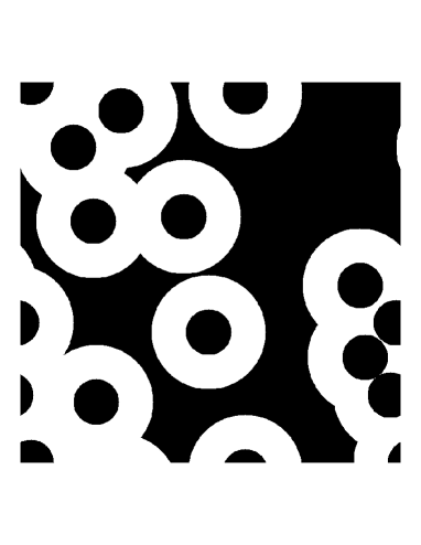
Figure 1: U. Brodatzki, K. Mecke, Morphological Model for Colloidal Suspensions

Figure 2

  

Figure 2: U. Brodatzki, K. Mecke, Morphological Model for Colloidal Suspensions

Figure 3

Figure 3: U. Brodatzki, K. Mecke, Morphological Model for Colloidal Suspensions

Figure 4

  

Figure 4: U. Brodatzki, K. Mecke, Morphological Model for Colloidal Suspensions

References

- [1] D. Beysens and D. Esteve, Phys. Rev. Lett. 54, 2123 (1985); T. Narayanan, A. Kumar, E. S. R. Gopal, D. Beysens, P. Guenoun, and G. Zalczer, Phys. Rev. E 48, 1989 (1993).
- [2] P. D. Gallagher and J. V. Maher, Phys. Rev. A 46, 2012 (1992); M. L. Kurnaz and J. V. Maher, Phys. Rev. E 51, 5916 (1995).
- [3] Y. Jayalakshmi and E. W. Kaler, Phys. Rev. Lett. 78, 1379 (1997).
- [4] D. Beysens, J. M. Petit, T. Narayanan, A. Kumar, and M. L. Broide, Ber. Bunsen-Ges. Phys. Chem. 98, 382 (1994).
- [5] H. T. Dobbs and J. M. Yeomans, J. Phys.: Condens. Matter 4, 10133 (1992).
- [6] H. Löwen, Phys. Rev. Lett. 74, 1028 (1995); Z. Phys. B 97, 269 (1995).
- [7] T. Gil, J. H. Ipsen, and C. F. Tejero, Phys. Rev. E 57, 3123 (1998).
- [8] L. A. Santalò, Integral Geometry and Geometric Probability (Addison - Wesley, Reading, MA, 1976).
- [9] H. Hadwiger, Vorlesungen über Inhalt, Oberfläche und Isoperimetrie, Springer (1957)
- [10] K. R. Mecke, Th. Buchert, and H. Wagner, Astron. Astrophys. 288, 697 (1994).
- [11] K. R. Mecke and H. Wagner, J. Stat. Phys. 64, 843 (1991).
- [12] J. P. Hansen and I. R. McDonald, Theory of simple liquids (Academic, London, 1986).
- [13] W. G. Hoover and F. H. Ree, J. Chem. Phys. 49, 3609 (1969).
- [14] K. Mecke J. Phys.: Condensed Matter 8, 9663 (1996).
- [15] Likos, C. N., K. Mecke, and H. Wagner, J. Chem. Phys. 102, 9350 (1995).