Cracks and Crazes: On calculating the macroscopic fracture energy of glassy polymers from molecular simulations

Abstract

We combine molecular dynamics simulations of deformation at the submicron scale with a simple continuum fracture mechanics model for the onset of crack propagation to calculate the macroscopic fracture energy of amorphous glassy polymers. Key ingredients in this multiscale approach are the elastic properties of polymer crazes and the stress at which craze fibrils fail through chain pullout or scission. Our results are in quantitative agreement with dimensionless ratios that describe experimental polymers and their variation with temperature, polymer length and polymer rigidity.

Understanding the molecular origins of macroscopic mechanical properties such as the fracture energy $G_{c}$ is a fundamental scientific challenge. In tough materials, the work $G_{c}$ required to propagate a crack through a unit area is orders of magnitude higher than the lower bound provided by the equilibrium interfacial free energy $G_{\rm eq}$ of the crack surfaces. Efforts to calculate this large increase in fracture energy have been frustrated, because phenomena on many length scales must be treated simultaneously [1]. In both amorphous and crystalline materials, the fracture energy depends on processes that range from breaking of atomic bonds to formation of defect structures on micron and larger scales.

In this Letter, we present a multiscale approach that allows us to calculate the plane strain fracture energy of an important class of unfilled amorphous polymer glasses. Experiments [4, 5, 6] show that under tensile loading the fracture energy of materials such as polystyrene (PS) and polymethylmethacrylate (PMMA) is mainly due to the formation of an intriguing craze structure in a “process zone” around the crack tip (Fig. 1). This results in a large increase in fracture energy, $G_{c}/G_{eq}\sim 10^{3}-10^{4}$, that is essential to the use of these materials as adhesives, packaging materials and windows [2, 3, 4].

In the craze, $\sim 0.5$nm diameter polymers are bundled into an intricate network of $\sim 10$nm diameter polymers that extends $\sim 10\mu$m on either side of the $\sim$ mm crack and $\sim 100\mu$m ahead of the crack tip. Molecular level simulations of regions with linear dimensions of mm or even $\mu$m are not feasible. They would also be inefficient, since most regions near the crack are homogeneous enough to be treated with continuum mechanics [5, 7]. Here, we combine the two approaches using molecular simulations of representative volume elements (see Fig. 1) to provide information about craze formation, deformation and failure that is needed to construct a continuum fracture mechanics model.

One advantage of studying polymeric systems is that many dimensionless ratios are independent of the specific chemistry of the molecules. For this reason we consider a bead-spring model that has been shown to provide a realistic description of polymer behavior [8, 9, 10, 11]. Each linear polymer contains $N$ beads of mass $m$. Van der Waals interactions between beads separated by a distance $r$ are modeled with a truncated Lennard-Jones potential: $V_{\rm LJ}(r)=4u_{0}\left[(a/r)^{12}-(a/r)^{6}-(a/r_{c})^{12}+(a/r_{c})^{6}\right]$ for $r\leq r_{c}=1.5\,a$, where $u_{0}$ and $a$ are characteristic energy and length scales. A simple analytic potential, $V_{\rm br}(r)=-k_{1}(r-r_{c})^{3}(r-R_{1})$, is used for the covalent bonds between adjacent beads along each chain. The constants $k_{1}$ and $R_{1}$ are adjusted to fix the equilibrium bond length [8], $0.96a$, and the ratio of the forces at which covalent and van der Waals bonds break. We find that this ratio is the only important parameter in the covalent potential and set it to 100 based on data for real polymers [11, 12]. The polymer rigidity and entanglement length $N_{e}$ are varied by introducing local bond-bending forces [10] with a potential $V_{B}=b\sum_{i=2}^{N-1}\left(1-\frac{(\vec{r}_{i-1}-\vec{r}_{i})\cdot(\vec{r}_{i}-\vec{r}_{i+1})}{|(\vec{r}_{i-1}-\vec{r}_{i})||(\vec{r}_{i}-\vec{r}_{i+1})|}\right)$ along the backbone. $\vec{r}_{i}$ denotes the position of the $i$th bead along the chain, and $b$ characterizes the stiffness. Two limiting cases of fully flexible $(N_{e}\sim 60-70$ beads, $b=0u_{0}$) and semiflexible $(N_{e}\sim 30$ beads, $b=1.5u_{0}$) chains are considered here. The chain length is varied from $N=64$ beads to $1024$ beads.

We first show that our model captures the essential experimental features of craze formation (Fig. 1A). The simulation cell has periodic boundary conditions and is initially a cube of size $L$. The length along one direction $L_{3}$ is increased at constant rate, while the other dimensions of the cell are held fixed. Fig. 2(a) shows typical results for the stress $\sigma_{3}$ along the stretching direction as a function of the elongation $L_{3}/L$. In all cases, there is an initial peak at small strains, where the material yields by cavitation [13, 14]. As in experiment [6], this peak is followed by a long plateau at a constant stress $S$. During this plateau, deformation is localized in a narrow “active zone” at the boundary of the growing craze network (Fig. 1A).

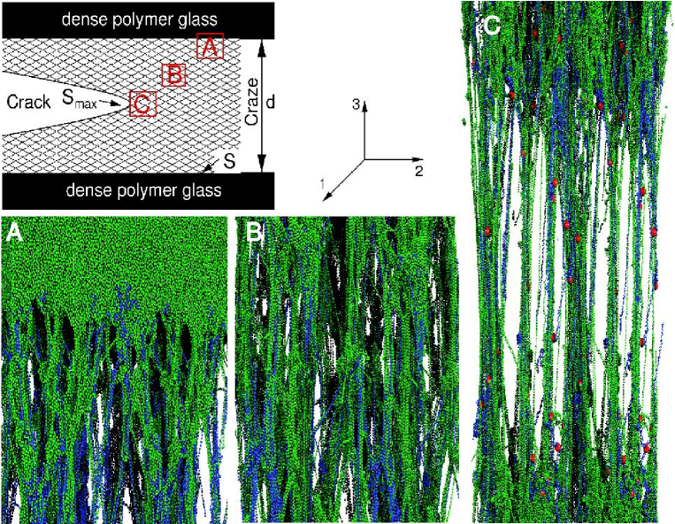
$S$ represents the stress needed to draw fibrils out of the dense regions adjacent to the craze [9]. This steady state drawing process increases the volume occupied by the polymer by a constant factor called the extension ratio $\lambda$. When $L_{3}/L$ reaches $\lambda$, the entire system has evolved into a craze, and the stress (Fig. 2(a)) begins to rise.

It is evident from Fig. 2(a) that $\lambda$ is strongly dependent on chain rigidity and thus the entanglement length $N_{e}$. We find that $\lambda$ decreases from about 6.1 for flexible chains to 3.6 for semiflexible chains. As in experiments, these values are quantitatively consistent with a simple model that assumes entanglements act like permanent chemical crosslinks [6]. During crazing, segments between entanglements are expanded from their equilibrium random-walk configurations to nearly straight lines (Fig. 1B).

We consider the common case where the dominant contribution to the fracture energy is the work needed to craze material in the process zone ahead of the crack tip[4]. As the crack advances, each region is expanded

at the constant plateau stress $S$. In steady state, advancing the crack over an area $A$ has the net effect of expanding a region of this area at constant stress from its initial width to the final width $d$ at which the craze cracks. Thus $G_{c}=S(d-d/\lambda)$ [15]. After normalizing by the lower bound for the fracture energy provided by the interfacial free energy change $G_{\rm eq}=2\gamma$, the fracture energy can be written in dimensionless form as

$$\frac{G_{c}}{G_{\rm eq}}=\frac{SD_{0}}{2\gamma}\frac{d}{D_{0}}(1-1/\lambda).$$ (1)

Eq. (1) shows that $G_{c}$ is primarily limited by the craze width $d$. Unlike the other quantities in Eq. (1), $d$ cannot be obtained directly from MD simulations. However, a minimal continuum model proposed by Brown [5] allows us to calculate $d$.

Brown pointed out that although there is a constant plateau stress $S$ on the craze boundary, a stress concentration occurs near the crack tip (see Fig. 1). He formulated a fracture criterion by equating the stress at the crack tip to the maximum stress $S_{\rm max}$ that the craze fibrils can withstand. The stress at a distance $r$ from a crack tip in a continuous elastic medium diverges as $r^{-1/2}$. This divergence is cut off at the characteristic fibril spacing $D_{0}$, below which the material can no longer be treated as a homogeneous elastic medium. Since the stress varies from $S_{\rm max}$ to $S$ as $r$ varies from $D_{0}$ to $d/2$, $S_{\rm max}\propto S\left(d/D_{0}\right)^{1/2}$. Solving the linear fracture mechanics problem within the craze yields [16]

$$\frac{d}{D_{0}}=4\pi\kappa\left(\frac{S_{\rm max}}{S}\right)^{2},$$ (2)

where $S_{\rm max}$ denotes the maximum stress that the craze fibrils can withstand, and the prefactor $\kappa$ depends on the anisotropic elastic constants $c_{ij}$ of the craze network (Eq. (3)). Neither the elastic properties of the craze network nor $S_{\rm max}$ are easily obtained from experiments. However, we can calculate both from MD simulations of regions B and C in Fig. 1 and thereby provide the key ingredients for calculating the fracture energy of glassy polymers from Eqs. (1) and (2).

Elastic constants were calculated by applying small ($\leq 0.5$%) step strains to fully developed crazes (Fig. 1B) at two different elongations $L_{3}/L$ and measuring the change in stress. Table I shows key ratios for flexible and semiflexible chains at two representative temperatures $T=0.1\,u_{0}/k_{B}$ and $T=0.01\,u_{0}/k_{B}$. Both are well below the glass transition temperature $T_{g}\approx 0.35\,u_{0}/k_{B}$ of the bead-spring model. As can be expected from the highly oriented structure of the craze network (see Fig. 1), $c_{33}$ is always much bigger than the other elastic constants, which are all of the same order. The prefactor $\kappa$ in Eq. (2) is given by [16]

$$\kappa^{2}=\frac{(1-C_{2})+(c_{33}/2c_{44})(1-C_{1})}{2(1-C_{1})^{2}},$$ (3)

where $C_{1}\equiv 2C_{2}c_{13}/c_{33}$ and $C_{2}\equiv c_{13}/(c_{11}+c_{12})$. Inserting the elastic constants, we obtain values for $\kappa$ between 2.0 and 2.8 for flexible chains and between 1.1 and 1.7 for semiflexible chains. The crazes with higher elongations always have a lower value of $\kappa$.

A simple approximate expression $\kappa\approx\sqrt{c_{33}/4c_{44}}$ can be obtained by noting that $c_{33}\gg c_{13}$, and thus $C_{1}\sim 0$ and $C_{2}\sim 1$. Table I also shows that this is an accurate approximation for all practical purposes. This simple expression shows clearly that the ability of crazes to resist shear $(c_{44}>0)$ limits their fracture energy. As first pointed out by Brown [5], the absence of lateral stress transfer would lead to $\kappa\rightarrow\infty$ and thus to an infinite $G_{c}$.

To determine the stress $S_{\rm max}$ at which fibrils break, we continue straining the fully developed craze until it fails (Fig. 1C). Although all chains that are long enough to form stable crazes ($N/N_{e}\gtrsim 2$ [9]) show the same plateau stress and extension ratio, their crazes exhibit very different behavior for $L_{3}/L>\lambda$ (Fig. 2(a)). Short chains of length $N/N_{e}=2$ easily pull free from the topological constraints imposed by entanglements, and the stress drops monotonically. As $N$ increases, the force needed to pull chains free from entanglements along a failure plane rises, and there is a corresponding increase in $S_{\rm max}$. The failure mechanism changes when the force needed to disentangle the chains reaches the breaking force for covalent bonds. At this point the forces along the chains and $S_{\rm max}$ both saturate due to chain scission.

FIG. 2.: (a) Normalized stress $\sigma_{3}/S$ during craze growth at $T=0.3\,u_{0}/k_{B}$ for flexible (solid lines) and semiflexible (dotted lines) chains of the indicated length in systems composed of 32768 beads. Here we take $N_{e}=32$ for the semiflexible and $N_{e}=64$ for the flexible chains. The value of $S_{\rm max}/S$ is obtained from the maximum height of the curves. Panel (b) summarizes $S_{\rm max}/S$ for the flexible ($\circ$) as well as semiflexible ($\triangle$) chains at $T=0.3\,u_{0}/k_{B}$ (open symbols) and $T=0.1\,u_{0}/k_{B}$ (filled symbols) as a function of chain length.

Fig. 2(b) summarizes our results for $S_{\rm max}/S$ as a function of chain length, temperature and flexibility. As $N/N_{e}$ rises above 2, $S_{\rm max}/S$ rises rapidly and then saturates due to the change in failure mechanism from chain pullout to chain scission. Saturation occurs for $N/N_{e}$ between 8 and 16. The limiting value of $S_{max}/S$ lies between 3.4-3.8 for $T\leq 0.1u_{0}/k_{B}$ and 5.0-5.3 for $T=0.3u_{0}/k_{B}$ and increases slightly with chain rigidity. In general, more chain scission is observed for chains with higher rigidity and at lower temperatures.

We are now in a position to evaluate Eq. (2) and compare our results to experimental values. For flexible chains, $\kappa=2.0-2.8$ and $S_{\rm max}/S=3.4-5.0$, yielding $d/D_{0}$ between 290 - 890. Values for semiflexible chains give $d/D_{0}$ between 200 - 600. Typical craze widths $d$ observed in experiments range between $3-20\,{\rm\mu m}$, whereas characteristic fibril spacings $D_{0}$ have values between $20-30\,{\rm nm}$. Thus the range of experimental values for $d/D_{0}=100-1000$ overlaps well with our results.

In addition to values quoted above, calculating the fracture energy from Eq. (1) requires values for the plateau stress $S$, mean fibril spacing $D_{0}$, and surface tension $\gamma$. Typical values from our simulations are $S=0.5-1.4\,u_{0}/a^{3}$, $D_{0}=10-14\,a$, and $\gamma=0.6-1.0\,u_{0}/a^{2}$. With these values, we arrive at our final result $G_{c}/G_{\rm eq}=1300-4300$ (flexible polymers) and $G_{c}/G_{\rm eq}=1200-3500$ (semiflexible polymers). Within this range, $G_{c}/G_{\rm eq}$ tends to drop with increasing chain rigidity and decreasing temperature $T$. This trend is also found in real adhesive joints, where the fracture energy generally decreases with decreasing temperature [2].

Our simulations agree with experimental observations in greater detail. Sha et. al. [17] have compiled values of $G_{c}$ for PS and PMMA as a function of polymer molecular weight $M_{w}$. Neither polymer shows a large fracture energy when $M_{w}$ is less than twice $M_{e}$. As in our simulations (Fig. 2(b)), the fracture energy rises rapidly as $M_{w}/M_{e}$ rises above 2 and then saturates around 10 $M_{e}$. The limiting values of $G_{c}/G_{eq}$ at large $M_{w}/M_{e}$, 2500 (PMMA) and 5000 (PS), are comparable to our predicted values.

In conclusion, we have demonstrated that supplementing a simple continuum model with constitutive relations from molecular simulations can provide quantitative predictions for key material parameters such as the fracture energy. This approach can be further developed by using chemically detailed interaction potentials for specific polymers in the molecular simulations. For example, one might expect that a realistic treatment of side groups could increase the friction between polymers during craze formation, and increase the likelihood of chain scission. A more detailed finite element model for crack propagation could also be used, as in recent work [18, 19] that assumed simple constitutive relations for craze widening and breakdown. Although one might hope to include all length scales simultaneously in a hybrid calculation, this is complicated by the rapid increase in the relevant time scale with increasing length scale [7]. Finally, it should be noted that macroscopic cracks can contain an ensemble of crazes with characteristic sizes and spacings and that other processes such as shear banding can contribute to the fracture energy, depending on loading conditions and materials. These issues should provide fruitful topics for future work.

This work was supported by the Semiconductor Research Corporation and National Science Foundation Grant 0083286. We thank H. R. Brown, E. J. Kramer, and C. Denniston for stimulating discussions.

TABLE I.: Elastic properties of model crazes composed of 262 144 beads with flexible (fl.) and semiflexible (sfl.) chains at two elongations $L_{3}/L$. Uncertainties in $c_{ij}$ are about 10%. Here $N=256$, but the results do not depend on $N$ for $N>2N_{e}$. They are also insensitive to the covalent bond potential, since strain is accommodated by the weaker van der Waals bonds.

	$T[u_{0}/k_{B}]$	$L_{3}/L$	$c_{11}/c_{33}$	$c_{44}/c_{33}$	$\kappa$	$\sqrt{c_{33}/4c_{44}}$
fl.	0.01	5.5	0.026	0.038	2.8	2.6
	0.01	7.9	0.016	0.065	2.0	2.0
	0.1	5.8	0.030	0.041	2.7	2.5
	0.1	7.9	0.015	0.054	2.2	2.1
sfl.	0.01	3.4	0.12	0.10	1.7	1.6
	0.01	4.8	0.051	0.10	1.6	1.6
	0.1	3.4	0.087	0.086	1.9	1.7
	0.1	4.8	0.026	0.15	1.4	1.3

REFERENCES

- [1] Materials Research by Means of Multiscale Computer Simulation, MRS Bulletin 26, No. 3 (2001)
- [2] R. P. Wool, Polymer Interfaces: Structure and Strength, (Hanser/Gardner, Munich, 1995).
- [3] A. V. Pocius, Adhesion and adhesives technology: an introduction, (Hanser/Gardner, Munich, 1997).
- [4] R. N. Haward, R. J. Young, Eds., The Physics of Glassy Polymers, (Chapman & Hall, London, 1997).
- [5] H. R. Brown, Macromolecules 24, 2752 (1991).
- [6] E. J. Kramer, L. L. Berger, Adv. Polymer Science 91/92,1 (1990).
- [7] F. F. Abraham, J. Q. Broughton, N. Bernstein, E. Kaxiras, Europhys. Lett. 44, 783 (1998); J. Q. Broughton, F. F. Abraham, N. Bernstein, E. Kaxiras, Phys. Rev. B 60, 2391 (1999).
- [8] M. Pütz, K. Kremer, G. S. Grest, Europhys. Lett. 49, 735 (2000).
- [9] A. R. C. Baljon, M. O. Robbins, Macromolecules 34, 4200 (2001).
- [10] R. Faller, F. Müller-Plathe, and A. Heuer, Macromolecules 33, 6602 (2000) and R. Faller and F. Müller-Plathe, ChemPhysChem. 2 , 180 (2001).
- [11] S. W. Sides, G. S. Grest, M. J. Stevens, Phys. Rev. E 64, 050802 (2001).
- [12] M. J. Stevens, Macromolecules 34, 1411 (2001); Macromolecules 34, 2710 (2001).
- [13] J. Rottler, M. O. Robbins, Phys. Rev. E 64, 051801 (2001).
- [14] A. R. C. Baljon, M. O. Robbins, Science 271, 482 (1996).
- [15] Since , this is equivalent to the result of the Dugdale model, which describes the shape of the crazed region assuming ideal plasticity [2].
- [16] P. C. Paris, G. C. Sih, Fracture Toughness Testing and its Applications, (American Society for Testing and Materials, Philadelphia, 1965) p. 60. The length of the process zone is assumed to be much larger than its width so that the craze boundaries are nearly parallel. Equation 2 is valid in the relevant limit of large . A more general expression is given by C. Creton, E. J. Kramer, H. R. Brown, and C.-Y. Hui, Adv. Polymer Sci. 156, 53 (2001).
- [17] Y. Sha, C. Y. Hui, A. Ruina, E. J. Kramer, Macromolecules 28, 2450 (1995).
- [18] M. G. A. Tijssens, E. van der Giessen, L. J. Sluys, Mechanics of Materials 32, 19 (2000); R. Estevez, M. G. A. Tijssens, E. van der Giessen, J. Mech. and Physics of Solids 48, 2585 (2000); M. G. A. Tijssens, E. van der Giessen, L. J. Sluys, Int. J. of Solids and Structures 37, 7307 (2000).
- [19] S. Socrate, M. C. Boyce, A. Lazzeri, Mech. Mater. 33, 155 (2001).