Huge Enhancement of Impurity Scattering due to Critical Valence Fluctuations in a Ce-Based Heavy Electron System

Recently, renormalization effect of impurity potential by quantum critical fluctuations has begun to attract much attention,${}^{\hbox{\immediate{\bf{?}},\penalty 1000\hskip 0.91003pt plus 0.70004pt minus 0.70004pt{\bf{?}},\penalty 1000\hskip 0.91003pt plus 0.70004pt minus 0.70004pt{\bf{?}},\penalty 1000\hskip 0.91003pt plus 0.70004pt minus 0.70004pt{\bf{?}},\penalty 1000\hskip 0.91003pt plus 0.70004pt minus 0.70004pt{\bf{?}},\penalty 1000\hskip 0.91003pt plus 0.70004pt minus 0.70004pt{\bf{?}},\penalty 1000\hskip 0.91003pt plus 0.70004pt minus 0.70004pt{\bf{?}})}}$ while the effect of impurities on the universality class of critical fluctuations was clarified quite long ago,${}^{\hbox{\immediate{\bf{?}})}}$ and that on the temperature dependence of the resistivity at quantum criticality has been discussed recently.${}^{\hbox{\immediate{\bf{?}})}}$ A theoretical guideline for discussing exactly such an effect has already been put forth more than three decades ago by Betbder-Matibet and Nozières in the framework of the Fermi liquid theory.${}^{\hbox{\immediate{\bf{?}})}}$ Indeed, they showed on the basis of the Ward identy that the impurity potenital, in one-component Fermi liquid, is renormalized by many-body effect in the forward scattering limit as

$${\tilde{u}}({\vec{k}}\to 0)={1\over z(1+F_{0}^{\rm s})}u({\vec{k}}\to 0),$$ (1)

where $u({\vec{k}})$ is the bare non-magnetic impurity potential and ${\tilde{u}}({\vec{k}})$ are the renormalized one, $z$ is the renormalization amplitude including all the manybody effects, and $F_{0}^{\rm s}$ the Landau parameter relevant to the correction of the charge susceptibility. For the potential of magnetic impurity, the relation similar to (1) holds with the Fermi liquid parameter $F_{0}^{\rm s}$ being replaced by $F_{0}^{\rm a}$ which gives the Fermi liquid correction of the spin susceptibility.

Heavy electron compound CeCu₂Ge₂ at ambient pressure changes drastically its electronic state at the pressure $P\simeq 17$GPa where the coefficient $A$ of $T^{2}$-term of the resistivity $\rho(T)$ decreases by about three orders of magnitude and the universal ratio $A/\gamma^{2}$, $\gamma$ being the Sommerfeld constant, changes from the value of heavy electorns to that of conventional $d$-band metals decreasing by 25 times.${}^{\hbox{\immediate{?})}}$ This suggests that the rapid valence change of Ce ion occurs at around that pressure. Indeed, the rapid volume change maintaining the crystal symmetry was observed at around the “critical” pressure by SOR-X ray diffraction implying that the rapid valence change occurs there.${}^{\hbox{\immediate{\bf{?}})}}$ It was also observed that the residual resistivity $\rho_{0}$ exhibits sharp peak at the same pressure.${}^{\hbox{\immediate{?})}}$ Similar behavior has been observed in CeRhIn₅ recently discovered pressure induce superconductor.${}^{\hbox{\immediate{\bf{?}})}}$ Recently, it was shown that $\rho_{0}$ can be enhanced through the renormalization of impurity potential by exchanging the critical valence fluctuations.${}^{\hbox{\immediate{?},\penalty 1000\hskip 0.91003pt plus 0.70004pt minus 0.70004pt{?},\penalty 1000\hskip 0.91003pt plus 0.70004pt minus 0.70004pt{\bf{?}})}}$ However, the argument is based on the perturbational treatment with the use of the phenomenological form of valence fluctuation propagator. A purpose of this Letter is to extend that treatment so as to take into account the full effect of vertex corrections to the impurity potenital on the basis of the Ward-Pitaevskii identity in two-component Fermi liquid. Namely, we derive a technically exact formula for the renormaliztion of impurity potential for the forward scattering associated with a rapid critical valence change in heavy electrons form the Kondo regime to the valence fluctuation one.

We start with an extended periodic Anderson model (PAM),

$$H=\sum_{p\sigma}\xi_{k}c_{p\sigma}^{\dagger}c_{p\sigma}+\epsilon_{\rm f}\sum_{p\sigma}f_{p\sigma}^{\dagger}f_{p\sigma}+U_{{\rm f}\textcompwordmark{\rm f}}\sum_{i}n_{i\uparrow}^{\rm f}n_{i\downarrow}^{\rm f}$$

$$\qquad+\sum_{p\sigma}(V_{p}c_{p\sigma}^{\dagger}f_{p\sigma}+{\rm h.c.})+U_{{\rm f}{\rm c}}\sum_{i\sigma\sigma^{\prime}}n_{i\sigma}^{\rm f}n_{i\sigma^{\prime}}^{\rm c},$$ (2)

where the conventional notations for PAM are used except for $U_{\rm fc}$, the f-c Coulomb repulsion. It has recently been shown that the effect of $U_{{\rm f}{\rm c}}$ is important for the rapid valence change to occur as the f-level $\epsilon_{\rm f}$ is increased approaching the Fermi level by the effect of pressure.${}^{\hbox{\immediate{\bf{?}},\penalty 1000\hskip 0.91003pt plus 0.70004pt minus 0.70004pt{\bf{?}})}}$ The one-particle Green function for a given spin direction in this system is given formally as

$$\left[G^{-1}_{ij}({\vec{p}},\varepsilon)\right]=\left[\begin{array}[]{cc}G_{{\rm f}{\rm f}}({\vec{p}},\varepsilon)&G_{{\rm f}{\rm c}}({\vec{p}},\varepsilon)\\ G_{{\rm c}{\rm f}}({\vec{p}},\varepsilon)&G_{{\rm c}{\rm c}}({\vec{p}},\varepsilon)\end{array}\right]^{-1}$$ (5)

$$=\left[\begin{array}[]{cc}\varepsilon-\epsilon_{{\rm f}}+\mu-\Sigma_{{\rm f}{\rm f}}({\vec{p}},\varepsilon)&-V_{p}-\Sigma_{{\rm f}{\rm c}}({\vec{p}},\varepsilon)\\ -V_{p}^{*}-\Sigma_{{\rm c}{\rm f}}({\vec{p}},\varepsilon)&\varepsilon-\xi_{\vec{p}}-\Sigma_{{\rm c}{\rm c}}({\vec{p}},\varepsilon)\end{array}\right],$$ (8)

where $\Sigma_{{\rm f}{\rm f}}$ is the selfenergy of f-electron and there also exist $\Sigma_{{\rm f}{\rm c}}$ and $\Sigma_{{\rm c}{\rm c}}$ as the many-body effect due to $U_{\rm ff}$ and $U_{\rm fc}$. It is noted that $G^{-1}_{ij}$ means $ij$-element of the inverse matrix of the Green function, e.g. $G^{-1}_{11}\neq G^{-1}_{{\rm f}{\rm f}}$ while $G_{11}=G_{{\rm f}{\rm f}}$.

For coupling to nonmagnetic impurities, the scattering matrix for this system is given generally as $u_{ij}({\vec{k}})=\sum_{a=1}^{4}u_{a}({\vec{k}})\lambda^{a}_{ij}$ where $u_{1}$ and $u_{2}$ are the variations of potential on f-electrons and c-electrons, respectively, while $u_{3}$ and $u_{4}$ represent the strength of the f-c mixing scattering. Here $\lambda^{a}_{ij}$ is the bare vertex for coupling to impurities and is given by $[\lambda^{1}_{ij}]=(1+\tau^{z})/2$, $[\lambda^{2}_{ij}]=(1-\tau^{z})/2$, $[\lambda^{3}_{ij}]=\tau^{x}/\sqrt{2}$ and $[\lambda^{4}_{ij}]=\tau^{y}/\sqrt{2}$ with ${\vec{\tau}}$ being the Pauli matrices in the f-c space.

In the following, a Greek index, e.g. $\alpha$, represents the dependence on both the component $i=1,2$ and the spin $\sigma=\uparrow,\downarrow$, and the summation is assumed to be taken for repeated indices. Then, the one-particle Green function and the scattering matrix mean the tensor product multiplied by the unit matrix with respect to the spin variables.

The Ward-Pitaevskii identity relevant to the present problem is given by considering the linear response of $G_{\gamma\alpha}$ caused by the shift of the parameter denoted by $\epsilon_{a}$ with the chemical potential $\mu$ being fixed. Here $\epsilon_{a}$ is the f-level $\epsilon_{\rm f}$, the center of the conduction band $\epsilon_{{\rm c}}$ or f-c mixing $V$, i.e., ${}^{t}[\epsilon_{a}]=(\epsilon_{1},\epsilon_{2},\epsilon_{3},\epsilon_{4})=(\epsilon_{\rm f},\epsilon_{{\rm c}},\sqrt{2}V^{\prime},\sqrt{2}V^{\prime\prime})$ with $V^{\prime}$ and $V^{\prime\prime}$ being the real and imaginary part of $V$, respectively. One can show, by anlyzing the structure of perturbation series of the selfenergy, that the following identity holds:

$$-{\hbox{$\left(\vbox to0.0pt{}\right.\n@space$}}\frac{\partial G_{\gamma\alpha}^{-1}(p)}{\partial\epsilon_{a}}{\hbox{$\left)\vbox to0.0pt{}\right.\n@space$}}_{\mu}=\lambda^{a}_{\gamma\alpha}+{\hbox{$\left(\vbox to0.0pt{}\right.\n@space$}}{\partial\Sigma_{\gamma\alpha}(p)\over\partial\epsilon_{a}}{\hbox{$\left)\vbox to0.0pt{}\right.\n@space$}}_{\mu}$$ (9)

$$=\lambda^{a}_{\gamma\alpha}-{\rm i}\int{{\rm d}^{4}q\over(2\pi)^{4}}\Gamma^{k}_{\gamma\delta,\alpha\beta}(p,q)\{G_{\beta\zeta}(q)G_{\kappa\delta}(q)\}_{k}\lambda^{a}_{\zeta\kappa}\quad$$ (10)

where $\Gamma^{k}$ is the so-called $k$-limit of the full vertex function, and $\{GG\}_{k}$ is the same limit of particle-hole Green function pair with the four-vector abbreviations $p=({\vec{p}},\varepsilon)$, etc. The process of renormalization of impurity potential is represented by the Feynman diagram as shown in Fig. 1. In the limit of forward scattering, i.e., $k\to 0$, the renormalized potential ${\tilde{u}}_{a}({\vec{k}})$ and the bare one $u_{a}({\vec{k}})$ are in the relation

$$\lim_{k\to 0}{\tilde{u}}_{a}({\vec{k}})=\lim_{k\to 0}\frac{1}{2}\lambda^{a}_{\alpha\gamma}u_{b}({\vec{k}})$$

$$\times{\hbox{$\left[\vbox to0.0pt{}\right.\n@space$}}\lambda^{b}_{\gamma\alpha}-{\rm i}\int{{\rm d}^{4}q\over(2\pi)^{4}}\Gamma^{k}_{\gamma\delta,\alpha\beta}(p,q)\{G_{\beta\zeta}(q)G_{\kappa\delta}(q)\}_{k}\lambda^{b}_{\zeta\kappa}{\hbox{$\left]\vbox to0.0pt{}\right.\n@space$}}.\quad\,\,$$ (11)

The reason why the $k$-limit vertex appears in (11) is that the impurity scattering is elastic maintaining the energy transfer $\omega=0$. Therefore, by the relation (10), the impurity potential is renormalized by $-(\partial G_{\gamma\alpha}^{-1}({\vec{p}},\varepsilon)/\partial\epsilon_{a})_{\mu}$ in the limit $k\to 0$.

In heavy electrons, the important effect of impurity on the quasiparticles arises from the variations of potential on f-electrons, because the quasiparticles consist mainly of f-electrons. Of these effects, those by displacement of non-f elements from the regular alignment around Ce ions is subject to remarkable renormalization by the critical valence fluctuations, because the impurity potential due to such effects is off the unitarity limit and has a space to be renormalized furthermore. On the other hand, the defect of Ce ions gives rise to the unitarity scattering from the beginning in heavy electron state so that its potential is subject only to a gradual renormalization with a weak anomaly around a possible transition point from the Kondo regime to VF one. It is noted that even if we consider only the effect of the shift of the f-level, i.e. in the case of $u_{2}=u_{3}=u_{4}=0$, the many-body effect due to $U_{{\rm f}{\rm c}}$ gives rise to the effective f-c and c-c scattering as can be seen in (11).

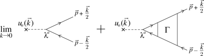
Fig.  1: Feynman diagram for the exact vertex correction of impurity potential $u({\vec{k}})$.

In the present system described by the Hamiltonian (2), the total number density of f-electrons and conduction electrons is conserved. This leads to the following identity:

$$\frac{\partial G^{-1}_{\gamma\alpha}(p)}{\partial\varepsilon}=\delta_{\gamma\alpha}-{\partial\Sigma_{\gamma\alpha}(p)\over\partial\varepsilon}$$ (12)

$$=\delta_{\gamma\alpha}-{\rm i}\int{{\rm d}^{4}q\over(2\pi)^{4}}\Gamma^{\omega}_{\gamma\delta,\alpha\beta}(p,q)\{G_{\beta\zeta}(q)G_{\zeta\delta}(q)\}_{\omega}\quad$$ (13)

where $\Gamma^{\omega}$ is the so-called $\omega$-limit of the full vertex function and $\{GG\}_{\omega}$ is the same limit of particle-hole Green function pair. The relation between $\Gamma^{k}$ and $\Gamma^{\omega}$ is given by

$$\Gamma^{k}_{\gamma\delta,\alpha\beta}(p,p^{\prime})=\Gamma^{\omega}_{\gamma\delta,\alpha\beta}(p,p^{\prime})-{\rm i}\int{{\rm d}^{4}q\over(2\pi)^{4}}\Gamma_{\gamma\kappa,\alpha\zeta}^{\omega}(p,q)$$

$$\times\left[\{G_{\zeta\xi}(q)G_{\eta\kappa}(q)\}_{k}-\{G_{\zeta\xi}(q)G_{\eta\kappa}(q)\}_{\omega}\right]\Gamma^{k}_{\xi\delta,\eta\beta}(q,p^{\prime}).\quad\quad$$ (14)

By using formulas (13) and (14), we can evaluate the left-hand side of (9) as shown below.

First, we write the total number density $n$ in terms of the Green function as

$$n=-{\rm i}\int{{\rm d}^{4}p\over(2\pi)^{4}}G_{\alpha\alpha}(p).$$ (15)

Differentiation of (15) with respect to $\epsilon_{a}$ with $\mu$ being fixed gives

$${\hbox{$\left(\vbox to0.0pt{}\right.\n@space$}}{\partial n\over\partial\epsilon_{a}}{\hbox{$\left)\vbox to0.0pt{}\right.\n@space$}}_{\mu}={\rm i}\int{{\rm d}^{4}p\over(2\pi)^{4}}\{G_{\alpha\beta}(p)G_{\beta\gamma}(p)\}_{k}{\hbox{$\left(\vbox to0.0pt{}\right.\n@space$}}\frac{\partial G_{\gamma\alpha}^{-1}(p)}{\partial\epsilon_{a}}{\hbox{$\left)\vbox to0.0pt{}\right.\n@space$}}_{\mu}.$$ (16)

By (10) and (14), we find the right hand side of (16) is

$${\rm i}\int{{\rm d}^{4}p\over(2\pi)^{4}}{\hbox{$\left[\vbox to0.0pt{}\right.\n@space$}}\delta_{\kappa\zeta}-{\rm i}\int{{\rm d}^{4}q\over(2\pi)^{4}}\{G_{\alpha\beta}(q)G_{\beta\gamma}(q)\}_{\omega}\Gamma^{\omega}_{\gamma\kappa,\alpha\zeta}(q,p){\hbox{$\left]\vbox to0.0pt{}\right.\n@space$}}$$

$$\times\left[\{G_{\zeta\xi}(p)G_{\eta\kappa}(p)\}_{k}-\{G_{\zeta\xi}(p)G_{\eta\kappa}(p)\}_{\omega}\right]{\hbox{$\left(\vbox to0.0pt{}\right.\n@space$}}\frac{\partial G_{\xi\eta}^{-1}(p)}{\partial\epsilon_{a}}{\hbox{$\left)\vbox to0.0pt{}\right.\n@space$}}_{\mu}$$

$$-{\rm i}\int{{\rm d}^{4}p\over(2\pi)^{4}}{\hbox{$\left[\vbox to0.0pt{}\right.\n@space$}}\delta_{\kappa\zeta}-{\rm i}\int{{\rm d}^{4}q\over(2\pi)^{4}}\{G_{\alpha\beta}(q)G_{\beta\gamma}(q)\}_{\omega}\Gamma^{\omega}_{\gamma\kappa,\alpha\zeta}(q,p){\hbox{$\left]\vbox to0.0pt{}\right.\n@space$}}$$

$$\times\{G_{\zeta\xi}(p)G_{\eta\kappa}(p)\}_{\omega}\lambda^{a}_{\xi\eta}.$$ (17)

According to the Ward identity (13), the integrand of the second term in (17) is just $\lambda_{\xi\eta}\partial G_{\eta\xi}({\vec{p}},\varepsilon)/\partial\varepsilon$ so that this term equals zero. Substituting (13) into the first term in (17), we obtain

$${\hbox{$\left(\vbox to0.0pt{}\right.\n@space$}}{\partial n\over\partial\epsilon_{a}}{\hbox{$\left)\vbox to0.0pt{}\right.\n@space$}}_{\mu}={\rm i}\int{{\rm d}^{4}p\over(2\pi)^{4}}\frac{\partial G_{\alpha\beta}^{-1}(p)}{\partial\varepsilon}{\hbox{$\left(\vbox to0.0pt{}\right.\n@space$}}\frac{\partial G_{\gamma\delta}^{-1}(p)}{\partial\epsilon_{a}}{\hbox{$\left)\vbox to0.0pt{}\right.\n@space$}}_{\mu}$$

$$\quad\quad\quad\times\left[\{G_{\beta\gamma}(p)G_{\delta\alpha}(p)\}_{k}-\{G_{\beta\gamma}(p)G_{\delta\alpha}(p)\}_{\omega}\right].\quad$$ (18)

Near the Fermi level, (5) is expressed in terms of quasiparticle as

$$G^{-1}_{ij}({\vec{p}},\varepsilon)\approx a^{-1}_{ij}({\vec{p}}\,)\varepsilon-\epsilon_{ij}({\vec{p}}\,),$$ (19)

where $a^{-1}_{ij}\equiv a^{-1}_{ij}({\vec{p}}\,)=\partial G^{-1}_{ij}({\vec{p}},\varepsilon)/\partial\varepsilon|_{\varepsilon=0}$ and $\epsilon_{ij}\equiv\epsilon_{ij}({\vec{p}}\,)$ is given by

$$\left[\epsilon_{ij}({\vec{p}}\,)\right]=\left[\begin{array}[]{cc}\epsilon_{{\rm f}}-\mu+\Sigma_{{\rm f}{\rm f}}({\vec{p}},0)&V+\Sigma_{{\rm f}{\rm c}}({\vec{p}},0)\\ V^{*}+\Sigma_{{\rm c}{\rm f}}({\vec{p}},0)&\xi_{\vec{p}}+\Sigma_{{\rm c}{\rm c}}({\vec{p}},0)\end{array}\right].$$ (20)

Then the one-particle Green function $G$ can be written in the form

$$G_{ij}({\vec{p}},\varepsilon)={\tilde{A}}_{ij}({\vec{p}}\,){\hbox{$\left/\vbox to0.0pt{}\right.\n@space$}}{\hbox{$\left[\vbox to0.0pt{}\right.\n@space$}}\varepsilon-{\tilde{E}}_{{\vec{p}}}^{-}{\hbox{$\left]\vbox to0.0pt{}\right.\n@space$}}+\mbox{nonsingular part},$$ (21)

where the renormalization amplitude ${\tilde{A}}_{ij}({\vec{p}}\,)$ and the dispersion of quasiparticles ${\tilde{E}}_{\vec{p}}^{\pm}$ near the Fremi level is given by

$${\hbox{$\left[\vbox to0.0pt{}\right.\n@space$}}{\tilde{A}}_{ij}({\vec{p}}\,){\hbox{$\left]\vbox to0.0pt{}\right.\n@space$}}={\rm det}\left(\hat{a}\right){\hbox{$\left/\vbox to0.0pt{}\right.\n@space$}}{\rm tr}\left(\hat{a}\hat{\epsilon}\right)$$

$$\quad\quad\times\left[\begin{array}[]{cc}\xi_{\vec{p}}+\Sigma_{{\rm c}{\rm c}}({\vec{p}},0)&-V-\Sigma_{{\rm f}{\rm c}}({\vec{p}},0)\\ -V^{*}-\Sigma_{{\rm c}{\rm f}}({\vec{p}},0)&\epsilon_{{\rm f}}-\mu+\Sigma_{{\rm f}{\rm f}}({\vec{p}},0)\end{array}\right],$$ (24)

$${\tilde{E}}_{\vec{p}}^{\pm}\equiv{1\over 2}\left[{\rm tr}\left(\hat{a}\hat{\epsilon}\right)\pm\sqrt{\left[{\rm tr}\left(\hat{a}\hat{\epsilon}\right)\right]^{2}-4{\rm det}\left(\hat{a}\hat{\epsilon}\right)}\right],$$ (25)

respectively, with $\hat{a}\equiv[a_{ij}]$ and $\hat{\epsilon}\equiv[\epsilon_{ij}]$. By (21), the differnce between the $k$-limit and the $\omega$-limit of the product $GG$ can be obtained to be

$$\{G_{ij}(p)G_{lm}(p)\}_{k}-\{G_{ij}(p)G_{lm}(p)\}_{\omega}$$

$$=-2\pi{\rm i}{\tilde{A}}_{ij}({\vec{k}}_{\rm F}){\tilde{A}}_{lm}({\vec{k}}_{\rm F})\delta({\varepsilon})\delta({\tilde{E}}_{\vec{p}}^{-}).$$ (26)

Substituting this equation into (18) and taking the summation of the spin variables, we obtain

$${\hbox{$\left(\vbox to0.0pt{}\right.\n@space$}}{\partial n\over\partial\epsilon_{a}}{\hbox{$\left)\vbox to0.0pt{}\right.\n@space$}}_{\mu}={\tilde{N}}_{\rm F}{\tilde{A}}_{ij}(k_{\rm F}){\hbox{$\left(\vbox to0.0pt{}\right.\n@space$}}\frac{\partial G_{ji}^{-1}(k_{\rm F},0)}{\partial\epsilon_{a}}{\hbox{$\left)\vbox to0.0pt{}\right.\n@space$}}_{\mu},$$ (27)

where ${\tilde{N}}_{\rm F}$ is the density of states of the quasi-particles. In deriving (27), we have used the relation ${\rm det}[{\tilde{A}}_{ij}(k_{\rm F})]=0$ so that ${\tilde{A}}_{ij}(k_{\rm F})a^{-1}_{jl}(k_{\rm F}){\tilde{A}}_{lm}(k_{\rm F})={\tilde{A}}_{im}(k_{\rm F})$. By virtue of (11), we finally find that the renormalized potential acting on the quasi-particles is given by

$${\tilde{A}}^{b}(k_{\rm F}){\tilde{u}}_{b}({\vec{k}}\to 0)=-\frac{1}{{\tilde{N}}_{\rm F}}{\hbox{$\left(\vbox to0.0pt{}\right.\n@space$}}{\partial n\over\partial\epsilon_{a}}{\hbox{$\left)\vbox to0.0pt{}\right.\n@space$}}_{\mu}u_{a}({\vec{k}}\to 0),$$ (28)

where ${\tilde{A}}^{b}(k_{\rm F})=\lambda^{b}_{ij}{\tilde{A}}_{ji}(k_{\rm F})$.

Equations (27) or (28) can be obtaind more easily in the limiting case of heavy electrons, $a_{{\rm f}}\equiv a_{11}\ll 1$, $a_{12}=a_{21}^{*}\sim 0$ and $a_{22}\sim 1$, which is the only way for the quasiparticle to acquire the extremely heavy mass. In such a case, the quasiparticles consist mainly of f-electrons whose weight in the quasiparticle state is given by $1-a_{{\rm f}}|V|^{2}/\xi_{k_{\rm F}}\approx 1$. Therefore, the derivative with respect to $\epsilon_{{\rm f}}$ in (9) is approximated in a high accuracy, neglecting $a_{{\rm f}}$ compared to 1, as

$$-{\partial\over\partial\epsilon_{{\rm f}}}G_{{\rm f}{\rm f}}^{-1}(p,\varepsilon){\hbox{$\left|\vbox to0.0pt{}\right.\n@space$}}_{\mu}$$

$$\qquad\approx{1\over a_{{\rm f}}}{\varepsilon-{\tilde{E}}_{k_{\rm F}}^{+}\over\varepsilon-\xi_{k_{\rm F}}}{\hbox{$\left|\vbox to0.0pt{}\right.\n@space$}}_{\varepsilon=0}\times(-1){\tilde{v}}_{k_{\rm F}}^{-}\left({\partial k_{\rm F}\over\partial\epsilon_{{\rm f}}}\right)_{\mu}$$ (29)

where the velocity of quasiparticles is defined as ${\tilde{v}}_{p}^{-}\equiv\partial{\tilde{E}}_{p}^{-}/\partial p$, and $p$ and $\varepsilon$ have been approximated by $p=k_{\rm F}$ and $\varepsilon=0$, respectively. In deriving (29), we have considered that the dispersion of quasiparticles near the Fermi level is approximated as ${\tilde{E}}_{p}^{\pm}\approx{\tilde{v}}_{p}^{-}(p-k_{\rm F})$ and

$$\lim_{p\to k_{\rm F}}\left({\partial{\tilde{E}}_{p}^{-}\over\partial\epsilon_{{\rm f}}}\right)_{\mu}=-{\tilde{v}}_{k_{\rm F}}^{-}\left({\partial k_{\rm F}\over\partial\epsilon_{{\rm f}}}\right)_{\mu}.$$ (30)

Since the renormalization factor $a_{{\rm f}}$ included in ${\tilde{v}}_{\rm F}^{-}$ and that in the denominator of (29) cancels with each other, we obtain

$$-{\partial\over\partial\epsilon_{{\rm f}}}G_{{\rm f}{\rm f}}^{-1}(p,\varepsilon){\hbox{$\left|\vbox to0.0pt{}\right.\n@space$}}_{\mu} \approx -v_{k_{\rm F}}\left({\partial k_{\rm F}\over\partial\epsilon_{{\rm f}}}\right)_{\mu}$$ (31)

$$\approx -{1\over N_{\rm F}}\left({\partial n_{{\rm f}}\over\partial\epsilon_{{\rm f}}}\right)_{\mu},$$ (32)

where $n_{{\rm f}}$ is the f-electron number density and $N_{\rm F}$ is the density of states of non-interacting electrons described by (2) at the Fermi level. The reason (31) is approximated by (32) is as follows: A variation of $k_{\rm F}$ under $\mu$ being fixed corresponds mainly to that of f-electron number, because the quasiparticles consist mainly of f-electrons${}^{\hbox{\immediate{\bf{?}})}}$ and the change of conduction-electron number is limited by the fixed chemical potential $\mu$. This physical picture can be verified on the basis of Gutzwiller approximation applied to PAM without $U_{{\rm f}{\rm c}}$.${}^{\hbox{\immediate{\bf{?}},\penalty 1000\hskip 0.91003pt plus 0.70004pt minus 0.70004pt{\bf{?}})}}$

By the relations (10), (11), and (32), the impurity potential acting on f-electrons, in the forward scattering limit, is renormalized by the valence fluctuations associated with the crossover from Kondo regime to VF one as

$${\tilde{u}}({\vec{k}}\to 0)\approx-{1\over N_{\rm F}}\left({\partial n_{{\rm f}}\over\partial\epsilon_{{\rm f}}}\right)_{\mu}u({\vec{k}}\to 0).$$ (33)

This is an anlog of the relation, (1), in which the factor $1/z(1+F_{0}^{\rm s})$ is reexpressed as $\chi_{\rm charge}/N_{\rm F}$. The relation (33) implies that the impurity scattering is critically enhanced if the valence of Ce-ion changes critically as the f-level $\epsilon_{{\rm f}}$ is tuned, relative to the Fermi level, by the pressures. Indeed, it has been demonstrated theoretically that the derivative $-(\partial n_{\rm f}/\partial\epsilon_{\rm f})_{n}$ can diverge in the system described by the model Hamiltonian (2) with appropriate values of $U_{\rm fc}$ and $\epsilon_{\rm f}$ .${}^{\hbox{\immediate{?},\penalty 1000\hskip 0.91003pt plus 0.70004pt minus 0.70004pt{?})}}$ This means $-(\partial n_{\rm f}/\partial\epsilon_{\rm f})_{\mu}$ also diverges there, because the following relation holds, up to the approximation (32),

$$\left({\partial n_{\rm f}\over\partial\epsilon_{\rm f}}\right)_{\mu}\approx{\displaystyle{\left({\partial n_{\rm f}\over\partial\epsilon_{\rm f}}\right)_{n}}\over\displaystyle{1-\left({\partial n_{\rm f}\over\partial n}\right)_{\epsilon_{\rm f}}}},$$ (34)

where the derivative $-(\partial n_{\rm f}/\partial n)_{\epsilon_{\rm f}}$ is a small number of the order of $z$, the renormalization amplitude.

In order to see how this enhancement of impurity potential affects the behaviors of the resistivity, we need to know the $k$-dependence of ${\tilde{u}}(k)$ for the scattering from ${\vec{p}}-{\vec{k}}/2$ to ${\vec{p}}+{\vec{k}}/2$ near the Fermi surface. Although it is not easy to determine the $k$-dependence accurately in general, it may be reasonbale to parameterize as

$${\tilde{u}}({\vec{k}})\approx{1\over\eta+Ak^{2}}u({\vec{k}}),$$ (35)

where $\eta$ is the inverse valence susceptibility, $\eta^{-1}\equiv|(\partial n_{{\rm f}}/\partial\epsilon_{{\rm f}})_{\mu}|/N_{\rm F}$, and $Ak_{\rm F}^{2}\sim{\cal O}(1)$. In the case where the bare impurity potential causes essentially the Born scattering, the enhancement of the residual resistivity $\rho_{0}$ by the critical fluctuations becomes gigantic. Indeed, $\rho_{0}$ is given as

$$\rho_{0}\approx\Biggl{\langle}{2\pi N_{\rm F}c_{\rm imp}|u({\vec{k}})|^{2}(1-\cos\theta)\over\bigl{[}\eta+A\bigl{(}2k_{\rm F}\sin^{2}(\theta/2\bigr{)}\bigr{]}^{2}}\Biggr{\rangle}_{\rm FS},$$ (36)

where $c_{\rm imp}$ is a concentration of impurity, $\theta$ is an angle between ${\vec{p}}\pm{\vec{k}}/2$, and the on-shell condition $\epsilon$=$\xi_{{\vec{p}}\pm{\vec{k}}/2}$=0 has been used. $\langle\cdots\rangle_{\rm FS}$ means that the average with respect to ${\vec{p}}$ over the Fermi surface is taken. Here it is noted that explicit dependence of renormalization amplitude does not appear due to cancellation between that for DOS and that for the damping rate of quasiparticles.${}^{\hbox{\immediate{\bf{?}})}}$ Calculation of angular average over $\theta$ is performed easily giving rise to

$$\rho_{0}\propto\ln{1\over\eta}.$$ (37)

This result remains valid even if we take into account higher order terms by calculating the $t$-matrix. It is because the scattering by the renormalized potential (33) is nothing but the Rutherford scattering in the limit of $\eta\to 0$.

It should be noted that the present result is not contradictory to the Friedel sum rule according to which the scattering probability does not diverge so long as the extra charge accumulated locally around the impurity is finite.${}^{\hbox{\immediate{\bf{?}},\penalty 1000\hskip 0.91003pt plus 0.70004pt minus 0.70004pt{\bf{?}})}}$ The form of renormalized impurity potential (33) becomes long ranged as $\eta\to 0$ even though the bare potential is short ranged. Namely, the change of valence near the impurity site extends in long range proportionally to $1/r$, $r$ being the distance from the impurity site. As a result, total amount of valence change around the impurity from that of the host metal is divergent while the local charge of f- and conduction electrons remains finite. So, the effect of impurity becomes long ranged making the scattering probability divergent.

The expression of $\rho_{0}$ given by (37) can explain a huge enhancement observed in CeCu₂Ge₂ and CeCu₂Si₂ at around the critical pressure where the rapid valence change seems to occur. This huge enhancement should be compared to the moderate enhancement around the magnetic quantum critical point where the enhancement arises only through the renormalization amplitude $z$ as discussed in Ref..${}^{\hbox{\immediate{?})}}$ The present mechanism of huge enhancement of $\rho_{0}$ is related to other systems near the quantum critical point associated with charge instability. For example, such a huge enhancement has been observed in Cd₂Re₂O₇ at around the pressure where the charge ordering temperature vanishies and the superconducting transition temperature $T_{\rm c}$ is considerably enhanced compared to that at the ambient pressure.${}^{\hbox{\immediate{\bf{?}})}}$ Similar enhancement is expected in $\beta$NaV₆O₁₅ which exhibits pressure induced superconductivity of $T_{\rm c}=10$ at around the pressure where the charge ordering is suppressed.${}^{\hbox{\immediate{\bf{?}})}}$

The enhancement of the two-dimensional charge sucseptibility was observed by photoemission spectroscopy near the metal-insulator transition in high-$T_{\rm c}$ cuprates LSCO.${}^{\hbox{\immediate{\bf{?}})}}$ This opens a new possibility that the doped ions, Sr ions in LSCO, which have only subtle influence on electrons in CuO₂ plane in the over and optimum regions, are transformed into the strong scattering center in the under doped region. Therefore, the carrier doping can suppress $T_{\rm c}$ of d-wave superconductivity considerably near the metal-insulator phase boundary.${}^{\hbox{\immediate{?})}}$

References

• [1] G. Kotliar, E. Abrahams, A. E. Ruckenstein, C. M. Varma, P. B. Littlewood and S. Schmitt-Rink: Europhys. Lett. 15 (1991) 655.
• [2] C. M. Varma: Phys. Rev. Lett. 97 (1997) 1535.
• [3] K. Miyake, O. Narikiyo and Y. Onishi: Physica B 259-261 (1999) 676.
• [4] K. Miyake and O. Narikiyo: preprint, cond-mat/0110174, submitted to J. Phys. Soc. Jpn.
• [5] D. Jaccard, E. Vargoz, K. Alami-Yadri and H. Wilhelm: Rev. High Pressure Sci. Technol. 7 (1998) 412; D. Jaccard, H. Wilhelm, K. Alami-Yadri and E. Vargoz: Physica B 259-261 (1999) 1.
• [6] C. Thessieu, J. Flouquet, G. Lapertot, A. N. Stepanov and D. Jaccard: Solid State Commun. 95 (1995) 707.
• [7] H. Maebashi, K. Miyake and C. M. Varma: preprint, cond-mat/0109276, submitted to Phys. Rev. Lett.
• [8] P. Fulde and A. Luther: Phys. Rev. 170 (1968) 570.
• [9] A. Rosch: Phys. Rev. Lett. 82 (1999) 4280, and references therein.
• [10] O. Betbeder-Matibet and P. Nozières: Ann. Phys. 37 (1966) 17.
• [11] A. Onodera: private communications.
• [12] T. Muramatsu et al: J. Phys. Soc. Jpn. 70 (2001) No.12, in press.
• [13] K. Miyake and H. Maebashi: J. Phys. Chem. Solids 62 (2001) 53.
• [14] Y. Onishi and K. Miyake: Physica B 281&282 (2000) 191.
• [15] Y. Onishi and K. Miyake: J. Phys. Soc. Jpn. 69 (2000) 3955.
• [16] A. A. Abrikosov, L. P. Gorkov and I. Ye. Dzyaloshinskii: Quantum Field Theoretical Methods in Satistical Physics, 2nd editions (Pergamon Press, Oxford, 1965) §19.3.
• [17] K. Yamada and K. Yosida: Prog. Theor. Phys. 76 (1986) 621.
• [18] T. M. Rice and K. Ueda: Phys. Rev. Lett. 55 (1985) 995; Phys. Rev. B 34 (1986) 6420.
• [19] P. Fazekas and B. H. Brandow: Phys. Scr. 36 (1987) 809.
• [20] J. S. Langer: Phys. Rev. 124 (1961) 1003.
• [21] J. Friedel: Phil. Mag. 43 (1952) 153; Nuovo Cimento Suppl. 7 (1958) 287.
• [22] J. S. Langer and V. Ambegaokar: Phys. Rev. 121 (1961) 1090.
• [23] Z. Hiroi: private communications.
• [24] T. Yamauchi: private communications.
• [25] A. Ino, T. Mizokawa, A. Fujimori, K. Tamasaku, H. Eisaki, S. Uchida, T. Kimura, T. Sasagawa and K. Kishio: Phys. Rev. Lett. 79 (1997) 2101.