Transition in the Fractal Properties from Diffusion Limited Aggregation to Laplacian Growth via their Generalization

Abstract

We study the fractal and multifractal properties (i.e. the generalized dimensions of the harmonic measure) of a 2-parameter family of growth patterns that result from a growth model that interpolates between Diffusion Limited Aggregation (DLA) and Laplacian Growth Patterns in 2-dimensions. The two parameters are $\beta$ which determines the size of particles accreted to the interface, and ${\cal C}$ which measures the degree of coverage of the interface by each layer accreted to the growth pattern at every growth step. DLA and Laplacian Growth are obtained at $\beta=0,~{}{\cal C}=0$ and $\beta=2,~{}{\cal C}=1$, respectively. The main purpose of this paper is to show that there exists a line in the $\beta-{\cal C}$ phase diagram that separates fractal ($D<2$) from non-fractal (D=2) growth patterns. Moreover, Laplacian Growth is argued to lie in the non-fractal part of the phase diagram. Some of our arguments are not rigorous, but together with the numerics they indicate this result rather strongly. We first consider the family of models obtained for $\beta=0,~{}{\cal C}>0$, and derive for them a scaling relation $D=2D_{3}$. We then propose that this family has growth patterns for which $D=2$ for some ${\cal C}>C_{\rm cr}$, where $C_{\rm cr}$ may be zero. Next we consider the whole $\beta-{\cal C}$ phase diagram and define a line that separates 2-dimensional growth patterns from fractal patterns with $D<2$. We explain that Laplacian Growth lies in the region belonging to 2-dimensional growth patterns, motivating the main conjecture of this paper, i.e. that Laplacian Growth patterns are 2-dimensional. The meaning of this result is that the branches of Laplacian Growth patterns have finite (and growing) area on scales much larger than any ultra-violet cut-off length.

I Introduction

In recent work 00BDLP ; 01BDP we have introduced a model of fractal growth processes that interpolates between Diffusion Limited Aggregation (DLA) 81WS and Laplacian Growth Patterns 58ST ; 84SB , and employed this model to show that these processes are not in the same universality classes. The aim of this paper is to study the fractal properties of the resulting clusters. In particular we will be led to conjecture that Laplacian Growth is asymptotically of dimension 2, and in this sense is not a fractal at all. This is in contradistinction to DLA for which the dimension had been computed to be 1.713…00DLP .

Laplacian Growth Patterns are obtained when the boundary $\Gamma$ of a 2-dimensional domain is grown at a rate proportional to the gradient of a Laplacian field $P$. Outside the domain $\nabla^{2}P=0$, and each point of $\Gamma$ is advanced at a rate proportional to ${\bf\nabla}P$ 58ST ; 84SB . In Diffusion Limited Aggregation (DLA) 81WS a 2-dimensional cluster is grown by releasing fixed size random walkers from infinity, allowing them to walk around until they hit any particle belonging to the cluster. Since the particles are released one by one and may take arbitrarily long time to hit the cluster, the probability field is quasi-stationary and in the complement of the cluster we have again $\nabla^{2}P=0$. The boundary condition at infinity is the same for the two problems; in radial geometry as $r\to\infty$ the flux is ${\bf\nabla}P={\rm const}\times\hat{r}/r$. Since the probability for a random walker to hit the boundary is again proportional to $|{\bf\nabla}P|$, one could think that in the asymptotic limit when the size of the particle is much smaller than the radius of the cluster, repeated growth events lead to a growth process which is similar to Laplacian Growth. Of course, the ultraviolet regularizations in the two processes were taken different; in studying Laplacian Growth one usually solves the problem with the boundary condition $P=\sigma\kappa$ where $\sigma$ is the surface tension and $\kappa$ the local curvature of $\Gamma$ 86BKT . Without this (or some other) ultraviolet regularization Laplacian Growth reaches a singularity (cusps) in finite time 84SB . In DLA the ultraviolet regularization is provided by the finite size of the random walkers. However, many researchers believed 84Pat that this difference, which for very large clusters controls only the smallest scales of the fractal patterns, were not relevant, expecting the two models to lead to the clusters with the same asymptotic dimensions. While we argued recently that the difference in ultraviolet regularization is indeed not crucial 01BDP , the two problems are nevertheless in two different universality classes. To establish this we have constructed a family of growth processes that includes DLA and a discrete version of Laplacian Growth as extreme members, using the same ultraviolet regularization (and see Sect. 2 for a further discussion of the regularization). We thus exposed the essential difference between DLA and Laplacian Growth. DLA is grown serially, with the field being updated after each particle growth. On the other hand all boundary points of a Laplacian pattern are advanced in parallel at once (proportional to ${\bf\nabla}P$). We showed that this difference is fundamental to the asymptotic dimension, putting the two problems in different universality classes 00BDLP . Here we wish to go further and suggest that Laplacian Growth patterns are 2-dimensional.

In Sect.2 we review briefly the two parameter model that had been introduced to establish these results. We discuss there the two parameters $\beta$ and ${\cal C}$ that are used to interpolate between DLA and Laplacian Growth. In Sect.3 we analyze the generalized dimensions $D_{q}$ and relate them to the scaling of moments of objects which are natural to the theory. In Sect. 4 we discuss first a family of growth models which is a 1-parameter generalization of DLA, ($\beta=0$, $0\leq{\cal C}\leq 1$, and show that the fractality of DLA is lost for some ${\cal C}>{\cal C}_{\rm cr}$ in favor of 2-dimensional growth patterns. It is not impossible that ${\cal C}_{\rm cr}=0$. For growth patterns in this family we derive a scaling relation $D=2D_{3}$. Under some plausible assumptions we propose that for ${\cal C}>{\cal C}_{cr}$ there exists another scaling relation, i.e. $D=1+D_{2}$, which implies immediatly that $D=2$. Secondly we discuss the 1-parameter family of models that generalizes Laplacian Growth ($\beta=2$, $0\leq{\cal C}\leq 1$ and show that the above relation is not obtained here, leading to the existence of fractal patterns also for high values of ${\cal C}$. Finally in Sect. 5 we reach the main conjecture of this paper, i.e. that Laplacian Growth patterns are 2-dimensional. In Sect. 6 we offer a discussion and some open questions that are left for future research.

II Iterated Conformal Maps for Parallel Growth Processes

The method of iterated conformal maps for DLA was introduced in 98HL . In 00BDLP ; 01BDP we have presented a generalization to parallel growth processes. We were interested in $\Phi^{(n)}(w)$ which conformally maps the exterior of the unit circle $e^{i\theta}$ in the mathematical $w$–plane onto the complement of the (simply-connected) cluster of $n$ particles in the physical $z$–plane. The unit circle is mapped onto the boundary of the cluster. In what follows we use the fact that the gradient of the Laplacian field ${\bf\nabla}P(z(s))$ is

$$|{\bf\nabla}P(z(s))|=\frac{1}{|{\Phi^{(n)}}^{\prime}(e^{i\theta})|}\ ,\quad z(s)=\Phi^{(n)}(e^{i\theta})\ .$$ (1)

Here $s$ is an arc-length parametrization of the boundary. The map $\Phi^{(n)}(w)$ is constructed recursively. Suppose that we have already $\Phi^{(n)}(w)$ which maps to the exterior of a cluster of $n$ particles in the physical plane and we want to find the map $\Phi^{(n+p)}(w)$ after $p$ additional particles were added to its boundary at once, each proportional in size to the local value of $|{\bf\nabla}P|^{\beta/2}$. To grow one such particle we employ the elementary map $\phi_{\lambda,\theta}$ which transforms the unit circle to a circle with a semi-spherical “bump” of linear size $\sqrt{\lambda}$ around the point $w=e^{i\theta}$:

$$\phi_{\lambda,0}(w)=\sqrt{w}\left\{\frac{(1+\lambda)}{2w}(1+w)\right.$$

$$\left.\times\left[1+w+w\left(1+\frac{1}{w^{2}}-\frac{2}{w}\frac{1-\lambda}{1+\lambda}\right)^{1/2}\right]-1\right\}^{1/2}$$ (2)

$$\phi_{\lambda,\theta}(w)=e^{i\theta}\phi_{\lambda,0}(e^{-i\theta}w)\,,$$ (3)

If we update the field after the addition of this single particle, then

$$\Phi^{(n+1)}(w)=\Phi^{(n)}(\phi_{\lambda_{n+1},\theta_{n+1}}(w))\ ,$$ (4)

where $\Phi^{(n)}(e^{i\theta_{n+1}})$ is the point on which the $(n+1)$-th particle is grown and $\sqrt{\lambda_{n}}$ is the size of the grown particle divided by the Jacobian of the map, ${\Phi^{{}^{\prime}(n)}}(e^{i\theta_{n+1}})$, at that point.

The map $\Phi^{(n+1)}(w)$ adds on a new semi-circular bump to the image of the unit circle under $\Phi^{(n)}(w)$. The bumps in the $z$-plane simulate the accreted particles in the physical space formulation of the growth process. For the height of the bump to be proportional to $|{\bf\nabla}P(z(s))|^{\beta/2}$ we need to choose its area proportional to $|{\Phi^{(n-1)}}^{\prime}(e^{i\theta_{n}})|^{-\beta}$ (see Eq. (1)), or

$$\lambda_{n}=\frac{\lambda_{0}}{|{\Phi^{(n-1)}}^{\prime}(e^{i\theta_{n}})|^{\beta+2}}\ .$$ (5)

With $\beta=0$ these rules produce a DLA cluster, for which the particles are of constant area. With $\beta=2$ we grow bumps in the physical space whose linear scale is proportional the gradient of the field $|{\bf\nabla}P(z(s))|$, as is appropriate for Laplacian Growth. Next, to grow $p$ (non-overlapping) particles in parallel, we accrete them without updating the conformal map. In other words, to add a new layer of $p$ particles when the cluster contains $m$ particles, we need to choose $p$ angles on the unit circle $\{\tilde{\theta}_{m+k}\}_{k=1}^{p}$. At these angles we grow bumps which in the physical space have the wanted linear scale (ranging from constant to proportional to the gradient of the field):

$$\lambda_{m+k}=\frac{\lambda_{0}}{|{\Phi^{(m)}}^{\prime}(e^{i\tilde{\theta}_{m+k}})|^{\beta+2}}\ ,\quad k=1,2\dots,p\ .$$ (6)

After the $p$ particles were added, the conformal map and thus the field should be updated. In updating, we will use $p$ compositions of the elementary map $\phi_{\lambda,\theta}(w)$. Of course, every composition effects a reparametrization of the unit circle, which has to be taken into account. To do this, we define a series $\{\theta_{m+k}\}^{p}_{k=1}$ according to

$$\Phi^{(m)}(e^{i\tilde{\theta}_{m+k}})\equiv\Phi^{(m+k-1)}(e^{i\theta_{m+k}})\ .$$ (7)

Next we define the conformal map used in the next layer growth according to

$$\Phi^{(m+p)}(\omega)\equiv\Phi^{(m)}\circ\phi_{\theta_{m+1},\lambda_{m+1}}\circ\dots\circ\phi_{\theta_{m+p},\lambda_{m+p}}(\omega)\ .$$ (8)

In this way we achieve the growth at the images under $\Phi^{(m)}$ of the points $\{\tilde{\theta}_{m+k}\}_{k=1}^{p}$. To compute the $\theta$ series from a given $\tilde{\theta}$ series we use Eq.(8) to rewrite Eq.(7) in the form

$$e^{i\theta_{m+k}}=\phi^{-1}_{\theta_{m+k-1},\lambda_{m+k-1}}\circ\dots\circ\phi^{-1}_{\theta_{m+1},\lambda_{m+1}}(e^{i\tilde{\theta}_{m+k}})$$ (9)

The inverse map $\phi^{-1}_{\theta,\lambda}$ is given by $\phi^{-1}_{\theta,\lambda}(\omega)=e^{i\theta}\phi^{-1}_{0,\lambda}(e^{-i\theta}\omega)$ with

$$\phi^{-1}_{0,\lambda}=\frac{\lambda\omega^{2}\pm\sqrt{\lambda^{2}\omega^{4}-\omega^{2}[1-(1+\lambda)\omega^{2}][\omega^{2}-(1+\lambda)]}}{1-(1+\lambda)\omega^{2}}\ ,$$ (10)

where the positive root is taken for Re $\omega>0$ and the negative root for Re $\omega<0$.

Evidently, Laplacian Growth calls for choosing the series $\{\tilde{\theta}_{m+k}\}_{k=1}^{p}$ such as to have full coverage of the unit circle (implying the same for the boundary $\Gamma$). On the other hand DLA calls for growing a single particle before updating the field. Since it was shown 99DHOPSS that in DLA growth $\lambda_{n}$ decreases on the average when $n$ increases, in the limit of large clusters DLA is consistent with vanishingly small coverage of the unit circle. To interpolate between these two cases we introduce a parameter that serves to distinguish one growth model from the other, giving us a 2-parameter control (the other parameter is $\beta$). This parameter is the degree of coverage. Since the area covered by the pre-image of the $n$-th particle on the unit circle is approximately $2\sqrt{\lambda_{n}}$, we introduce the parameter

$${\cal C}=\frac{1}{\pi}\sum_{k=1}^{p}\sqrt{\lambda_{m+k}}\ .$$ (11)

(In 01BDP we showed how to measure the coverage exactly). Since this is the fraction of the unit circle which is covered in each layer, the limit of Laplacian Growth is obtained with ${\cal C}=1$. DLA is asymptotically consistent with ${\cal C}=0$. Of course, the two models differ also in the size of the growing bumps, with DLA having fixed size particles, ($\beta=0$ in Eq.(5)), and Laplacian Growth having particles proportional to ${\bf\nabla}P$ ($\beta=2$ in Eq.(6)). Together with ${\cal C}$ we have a two parameter control on the parallel growth dynamics, with DLA and Laplacian Growth occupying two corners of the $\beta,{\cal C}$ plane, at the points (0,0) and (2,1) respectively.

Obviously, the partially serial growth within the layer introduces an additional freedom which is the order of placement of the bumps on the unit circle. In 00BDLP ; 01BDP we have shown that the order is in fact immaterial as far as the asymptotic fractal properties of the clusters are concerned. Accordingly, we will take random choices of $\tilde{\theta}_{m+k}$ with a rule of skipping overlaps.

We should note that in our approach the regularization of putative singularities is not achieved with surface tension, but by having a minimal size bump, similarly to the regularization of DLA. Our rules of growth with $\beta=2$ and $\lambda_{0}$ chosen once and for all, guarantee that every layer of growth has exactly the same area. This in the continuous time Laplacian Growth model translates to a particular choice of the time step $dt$. Clearly, one has freedom in choosing $dt$, or of the size $\lambda_{0}$ in each layer, as long as this does not affect the nature of the growth. In particular we can have $\lambda_{0}$ chosen such that the maximal physical bump is of constant area. Once $\lambda_{0}$ is chosen, the sharpest feature that can be achieved is a bump of size $\lambda_{0}$, and the worst possible “singularity” is a line of such bumps, exactly as in DLA. Thus the putative cusp singularity of Laplacian Growth is avoided in a manner that is identical for all the growth models in our 2-parameter family.

The conformal map $\Phi^{(n)}(\omega)$ admits a Laurent expansion

$$\Phi^{(n)}(\omega)=F_{1}^{(n)}\omega+F_{0}^{(n)}+\frac{F_{-1}^{(n)}}{\omega}+~{}\cdots\ .$$ (12)

The coefficient of the linear term is the Laplace radius, and was shown to scale like

$$F_{1}^{(n)}\sim S^{1/D}\ ,$$ (13)

where $S$ is the area of the cluster,

$$S=\sum_{j=1}^{n}\lambda_{j}~{}|{\Phi^{{}^{\prime}(j-1)}}(e^{i\theta_{j}})|^{2}\ .$$ (14)

Note that for $\beta=0$ this and equation (5) imply that $S=n\lambda_{0}$. Indeed for $\beta=0$ this estimate had been carefully analyzed and substantiated (up to a factor) in 2001SL . On the other hand $F_{1}^{(n)}$ is given analytically by

$$F_{1}^{(n)}=\prod_{k=1}^{n}\sqrt{(1+\lambda_{k})}\ ,$$ (15)

and therefore can be determined very accurately.

The conclusion from the calculations presented in 00BDLP ; 01BDP is that for ${\cal C}>0$ the fractal dimension of the growth patterns depends continuously on the parameters, growing monotonically upon decreasing $\beta$ or increasing ${\cal C}$. It is quite obvious why increasing ${\cal C}$ should increase the dimension. By forbidding particles to overlap we simply force them into the fjords, not allowing them to hit the tips only (as is highly probable). Also decreasing $\beta$ increases the dimension, since we grow larger particles into the fjords, whereas increasing $\beta$ reduces the size of particles added to fjords and increases the size of particles that accrete onto tips. In particular we argued that DLA and our discretized Laplacian Growth cannot have the same dimensions, putting them in different universality classes. In the rest of this paper we make these observations more quantitative and precise.

III Multifractal Properties

III.1 Generalized Dimensions

The fractal dimension in the $\beta-{\cal C}$ family of models, $D(\beta,C)$, is introduced as the exponent relating the area of the cluster $S_{n}$ to its linear scale (which is measured by the (dimensionless) Laplace radius $F_{1}^{(n)}$):

$$S_{n}\sim(F_{1}^{(n)})^{D(\beta,C)}\tilde{\lambda}_{0}\ .$$ (16)

In this equation $\tilde{\lambda}_{0}\equiv\lambda_{0}^{2/(2+\beta)}$. The multifractal exponents 83HP are defined in analogy to those for DLA in terms of the moments of the (dimensionless) electric field $E(s)$ on the boundary of the cluster 86HMP ,

$$\langle E^{(q-1)}\rangle \sim (F_{1}^{(n)})^{-(q-1)D_{q}(\beta,C)}$$ (17)

$$\sim (S_{n}/\tilde{\lambda}_{0})^{-(q-1)D_{q}(\beta,C)/D(\beta,C)},$$

where $\langle\cdots\rangle$ represents the harmonic average for the $(\beta,C)$ clusters in question. Note that these exponents are for a fixed size partition with boxes of length $\sqrt{\tilde{\lambda}_{0}}$, with asymptotics for an infinitely large cluster. A supremum over arbitrary partitions may lead to different exponents, cf. 86HJPKS .

This result translates immediately 99DHOPSS to the multifractal fluctuations of the bump areas $\lambda_{n}$ added in the mathematical plane. As $\lambda_{n}^{q}\sim E_{n}^{(2+\beta)q}$, where $E_{n}$ is the field computed at $z(s)=\Phi^{(n)}(e^{i\theta_{n}})$. We therefore write

$$\langle\lambda_{n}^{q}\rangle\sim(S_{n}/\tilde{\lambda}_{0})^{-(2+\beta)qD_{(2+\beta)q+1}(\beta,C)/D(\beta,C)}.$$ (18)

Specifically we can derive the following important moments

$$\langle\sqrt{\lambda_{n}}\rangle \sim (S_{n}/\tilde{\lambda}_{0})^{-(1+\beta/2)D_{(2+\beta/2)}/D}$$

$$\langle\lambda_{n}\rangle \sim (S_{n}/\tilde{\lambda}_{0})^{-(2+\beta)D_{3+\beta}/D}$$ (19)

$$\langle\lambda_{n}^{\beta/(2+\beta)}\rangle \sim (S_{n}/\tilde{\lambda}_{0})^{-\beta D_{1+\beta}/D}$$

where naturally all the dimensions are functions of $(\beta,C)$. We can also estimate the way in which the maximal bump areas scale

$$\lambda_{n,max}\equiv\lim_{q\to\infty}\langle\lambda_{n}^{q}\rangle^{1/q}\sim(S/\tilde{\lambda}_{0})^{-(2+\beta)D_{\infty}(\beta,C)/D(\beta,C)}.$$ (21)

Consider now the addition of one layer of $p$ particles to the growing cluster. We can rewrite Eq. (11) as

$$C=(1/\pi)p\overline{\sqrt{\lambda_{n}}},$$ (22)

where we have introduced the notation $\overline{\lambda_{n}^{q}}$ to represent the average over a layer of $p$ particles:

$$\overline{f(\lambda_{n})}\equiv\frac{1}{p}\sum_{k=1}^{p}f(\lambda_{n+k})$$ (23)

For our considerations below it is important to relate the layer averages $\overline{\lambda_{n}^{q}}$ to harmonic averages $\langle\lambda_{n}^{q}\rangle$. This relationship may very well depend on the value of $\beta$. The two case that are of highest interest to us are $\beta=0$ and $\beta=2$, and we will examine them separately.

IV Scaling relations for the Fractal Dimension $D$

IV.1 The case $\beta=0$ and ${\cal C}>0$

We examine the relationship between layer and harmonic averages numerically. In Fig. 1 we show the two averages vs. the number of layers for the case $q=1$, $\beta=0$ and four values of ${\cal C}$. In Fig. 2 we show the same for the case $q=0.5$, $\beta=0$ and the same four values of ${\cal C}$.

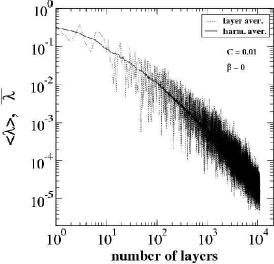
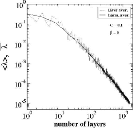
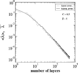
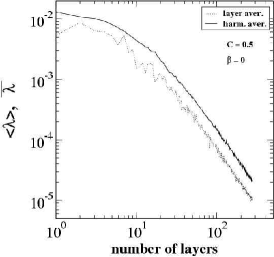
Figure 1: Layer and harmonic averages of $\lambda_{n}$ as a function of the number of layers, for $\beta=0$. Panels a-d: ${\cal C}=0.01,0.1,0.3$ and 0.5 respectively.

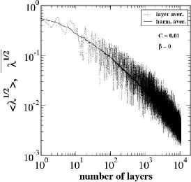
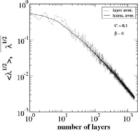
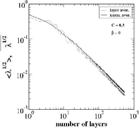
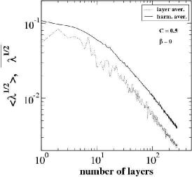
Figure 2: Layer and harmonic averages of $\lambda^{0.5}_{n}$ as a function of the number of layers, for $\beta=0$. Panels a-d: ${\cal C}=0.01,0.1,0.3$ and 0.5 respectively.

Examining the results it appears that for the higher values of ${\cal C}$ we can assume that in the scaling sense

$$\overline{\lambda_{n}^{q}}\sim\langle\lambda_{n}^{q}\rangle\ ,\quad\beta=0\ .$$ (24)

Note that for smaller values of ${\cal C}$ the evidence is not as clear cut as for higher values. The number of points $p$ in each layer is relatively small and the layer average is highly fluctuating. Nevertheless, even for the case ${\cal C}=0.01$, if we perform a running average on the layer average data, we converge very well onto the harmonic average. We therefore propose to proceed with the conjecture that Eq. (24) is correct for all the values of ${\cal C}$ and $\beta=0$, and investigate the implications of this scaling relation for the cases for which it is correct. An immediate consequence of Eqs. (22) and (24) is that

$$p\sim{\cal C}/\langle\sqrt{\lambda_{n}}\rangle\sim{\cal C}(S/\tilde{\lambda}_{0})^{D_{2}/D}$$ (25)

We note that this means that $p\to\infty$ asymptotically for every value of ${\cal C}$, while $p/n\to 0$.

Next observe that by definition

$$F_{1}^{(n+p)}/F_{1}^{(n)}=\Pi_{k=1}^{p}(1+\lambda_{n+k})^{a}\approx 1+ap\overline{\lambda_{n}}\ .$$ (26)

In light of Eq. (16) we write

$$\frac{S_{n+p}}{S_{n}}=\left(\frac{F_{1}^{(n+p)}}{F_{1}^{(n)}}\right)^{D}\approx 1+aDp\overline{\lambda_{n}}\ .$$ (27)

On the other hand we estimate

$$\frac{S_{n+p}}{S_{n}}\approx 1+\frac{p\tilde{\lambda}_{0}}{S_{n}}\ ,$$ (28)

and comparing with (27) we find

$$S_{n}\approx\frac{\tilde{\lambda}_{0}}{aD\overline{\lambda_{n}}}\ .$$ (29)

If Eq.(24) is used, we find finally

$$S_{n}\approx\tilde{\lambda}_{0}\left(\frac{S_{n}}{\tilde{\lambda}_{0}}\right)^{2D_{3}/D}\ .$$ (30)

from which we derive the well known “electrostatic relation”

$$D=2D_{3}\ .$$ (31)

This result was known for ${\cal C}=0$ 94Hal , and is generalized here, under the conjecture (24) to all values of ${\cal C}$.

Let us consider now the probability to hit at the point of maximal radius. We propose that for any finite ${\cal C}$ the probability for this event is finite. We stress that this “point” is actually a region on the interface of size $\sqrt{\tilde{\lambda}_{0}}$ in every layer. In particular, we expect that the growth process will hit the point of maximal radius every finite number of layers, where this number is of the order of $1/{\cal C}$. We also know for sure that we have at most one hit per layer since particles cannot overlap in the dynamics.

Consider now the scaling of the size of the growth pattern which is measured by $F_{1}^{(n)}$. First we know that $F_{1}^{(n)}\sim(S/\tilde{\lambda}_{0})^{1/D}$, and therefore

$$dF_{1}^{(n)}/dS\sim(S/\tilde{\lambda}_{0})^{1/D-1}/\tilde{\lambda}_{0}\ .$$ (32)

On the other hand, we estimate the same object using the following argument: the maximal radius $R^{(n)}$ increases by $\sqrt{\tilde{\lambda}_{0}}$ every time that it is hit. This occurs every $1/{\cal C}$ layers in which $p$ particles were added. Therefore

$$\frac{dR^{(n)}}{dS}\sim\frac{\sqrt{\tilde{\lambda}_{0}}}{p{\tilde{\lambda}_{0}}/{\cal C}}$$ (33)

Comparing Eqs. (32) and (33), using Eq. (25) we obtain the scaling relation

$$D=1+D_{2}$$ (34)

Using the inequalities between the generalized dimensions and Eq. (31) we write

$$D-1=D_{2}\geq D_{3}=D/2\quad{\rm for~{}all}~{}{\cal C}>{\cal C}_{\rm cr}\ ,$$ (35)

which is equivalent to

$$D=2\quad{\rm for~{}all}~{}{\cal C}>{\cal C}_{\rm cr}$$ (36)

In other words, we conclude that along the line $\beta=0$ in the phase diagram $\beta-{\cal C}$, there exists a transition to growth patterns of dimension 2.

Since our arguments are not rigorous and the result quite surprising, we will examine the assumptions using an additional consideration. From Eqs. (34) and (35) follows that $D_{2}=1$, and from Eq. (25) it then follows that $p$ scales like

$$p\sim S^{1/2}\ ,\quad{\cal C}>{\cal C}_{\rm cr}\ .$$ (37)

This prediction is examined directly in Fig. 3. We see that it is obeyed extremely well for all the values of ${\cal C}\geq 0.1$, and it is not in contradiction with the data even for ${\cal C}=0.01$. We therefore cannot exclude the possibility that ${\cal C}_{\rm cr}=0$.

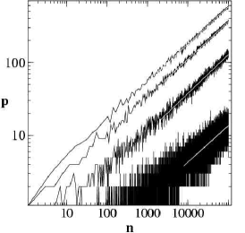
Figure 3: The number $p$ of bumps in a layer vs. the number $n$ of bumps in the growth pattern, in a log-log plot. From top to bottom that is shown for ${\cal C}=0.5$, 0.3, 0.1 and 0.01 respectively. In white lines we show the scaling laws $p\sim n^{1/2}$; this law fits the data for ${\cal C}\geq 0.1$ and is not in contradiction with the (noisy) data even for ${\cal C}=0.01$.

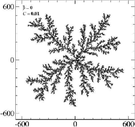
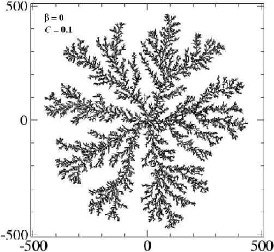
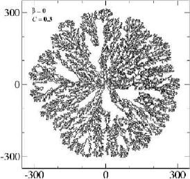
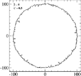
Figure 4: Clusters for $\beta=0$. Panels a-d: ${\cal C}=0.01,0.1,0.3$ and 0.5 respectively. Note the areas significantly larger than the UV-cutoff $\lambda_{0}$ which appear already for ${\cal C}=0.01$.

To gain intuition to the meaning of this result we show in Fig. 4 the actual growth patterns for $\beta=0$ and ${\cal C}=0.01$, 0.1, 0.3 and 0.5 respectively. To plot these figures we find all the exposed branch cuts on the unit circles which are associated with the bumps added in the growth process (see 01BDP for details). Then we plot the image of all these points under the conformal map and connect them by lines. Thus we are guaranteed that what is plotted is the actual contour of the growth pattern, of the image of the unit circle in the mathematical domain, with all the fjords fully resolved. We see that even with the lowest value of ${\cal C}$ the branches appear to gain substance as they grow, having a width which is larger than $\sqrt{\lambda_{0}}$ (the typical corrugation of the interface). Consequently it is not impossible that $D=2$ even for the lowest values of ${\cal C}>0$. If this is so, it is NOT due to the existence of an ultraviolet cutoff, but due to the finiteness of ${\cal C}$. With ${\cal C}=0$ (the DLA limit) the serial algorithm favors strongly truly fractal patterns. The parallel growth algorithm with finite ${\cal C}$ squeezes more substance into the fjords, reducing that tendency. For higher values of ${\cal C}$ it becomes obvious that the growth patterns are 2-dimensional, and for ${\cal C}=0.5$ the pattern grows like a roughened disk. The main conclusion of this analysis is that we certainly cross somewhere along the line $\beta=0$ into growth patterns that are 2-dimensional. Whether or not the critical value of ${\cal C}$ is finite or zero cannot be determined by numerics alone.

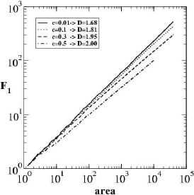
Figure 5: The first Laurent coefficient $F_{1}^{(n)}$ as a function of the area for $\beta=0$ and ${\cal C}=0.01,0.1,0.3$ and 0.5. The fractal dimension $D$ is obtained for the slope via $F_{1}^{(n)}\sim\sqrt{\lambda_{0}}(S/\lambda_{0})^{1/D}$

If we accept the possibility that even the lowest values of ${\cal C}$ are associated with growth patterns that are 2-dimensional, then we should stress that standard ways of estimating the dimension of these clusters, especially for the lowest value of ${\cal C}$, may fail to discover this fact. For example, we can compute $F_{1}^{(n)}$ and then, using Eq.(13), attempt to extract the dimension from log-log plots or $F_{1}^{(n)}$ against $S$. This method works very well for the fractal case, but it does not appear to do so well for the cases at hand. In Fig. 5 we show such log-log plots for all the clusters of Fig. 4. We see that even with 100 000 particles the dimension estimate is way below the suspected $D=2$, except for ${\cal C}=0.5$. In fact, any practitioner in the fractal field would be happy to interpret the scaling obtained for ${\cal C}=0.01$ as an indication that it is in the same universality class of DLA with dimension very close to $D=1.71$. While we cannot state confidently that for ${\cal C}=0.01$ the growth pattern is 2-dimensional, we stress that the dimension estimates obtained from log-log plots can be only taken as lower bounds on the true dimension, and these may not be very sharp.

A possibly better way to measure the dimension would be through the result (34) when it holds. We have very good methods to determine the correlation dimension $D_{2}$, going back to the Grassberger-Procaccia algorithm 83GP . To this aim we choose randomly $m=100000$ points $\{\theta_{i}\}_{i=1}^{m}$, and compute their positions on the interface of the cluster $z_{i}=\Phi^{(n)}(e^{i\theta_{i}})$. Next we compute the correlation integral

$$C^{(2)}(r)=\sum_{i\neq j}\Theta(|z_{i}-z_{j}|-r)\ ,$$ (38)

where $\Theta(x)$ is the step function, being 1 for $x\leq 0$ and 0 for $x>0$. The correlation integral is known to scale according to

$$C^{(2)}(r)\sim r^{D_{2}}\ .$$ (39)

In Fig. 6 we display this object in a log-log plot as a function of $r$. All the values of ${\cal C}$ agree with a correlation dimension of $D_{2}=1$, as can be seen from the plots at small scales. For those values of ${\cal C}$ for which Eq. (34) is correct this leads to the aforementioned result $D=2$.

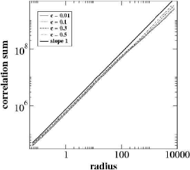
Figure 6: The correlation dimension $D_{2}$ for $\beta=0$ and ${\cal C}=0.01,0.1,0.3$ and 0.5. The thick line has slope 1, indicating that $D_{2}=1$ and therefore $D=2$ for all shown ${\cal C}$.

IV.2 The case $\beta=2$ and ${\cal C}>0$

The next interesting family of growth patterns that we focus on is obtained for $\beta=2$ and ${\cal C}>0$, with Laplacian Growth expected to be realized for ${\cal C}=1$. We find that for $\beta>0$ the numerics does not support the scaling relation (24). In Figs. (7) and (8) we show the layer and harmonic averages for $\beta=2$, and it is obvious that in this case

$$\overline{\lambda_{n}^{q}}\leq\langle\lambda_{n}^{q}\rangle$$ (40)

in the scaling sense.

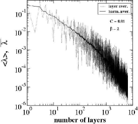
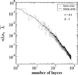
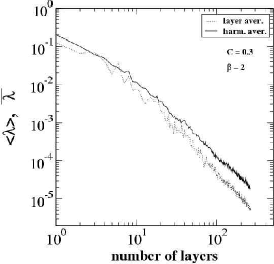
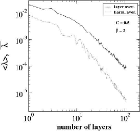
Figure 7: Layer and harmonic averages of $\lambda_{n}$ as a function of the number of layers, for $\beta=2$. Panels a-d: ${\cal C}=0.01,0.1,0.3$ and 0.5 respectively.

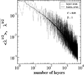
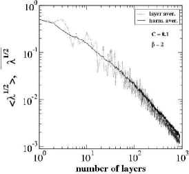
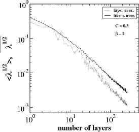
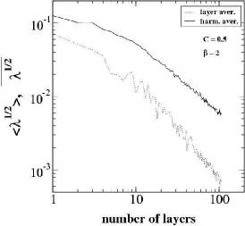
Figure 8: Layer and harmonic averages of $\lambda^{0.5}_{n}$ as a function of the number of layers, for $\beta=2$. Panels a-d: ${\cal C}=0.01,0.1,0.3$ and 0.5 respectively.

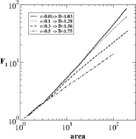
Figure 9: The first Laurent coefficient $F_{1}^{(n)}$ as a function of the area for $\beta=2$ and ${\cal C}=0.01,0.1,0.3$ and 0.5. The fractal dimension $D$ is obtained for the slope via $F_{1}^{(n)}\sim\sqrt{\tilde{\lambda}_{0}}(S/\tilde{\lambda}_{0})^{1/D}$

Once we have lost the scaling relation (24) we cannot argue that $D=2$ for any value of ${\cal C}>0$. We will find numerically that along the line $\beta=2$ we indeed find fractal patterns, (and cf. the next section); nevertheless even along this line there exists a transition to 2-dimensional patterns, albeit at a finite and rather high value of ${\cal C}$. Next we want to estimate this value.

V Conjecture: Laplacian Growth is 2-Dimensional

In this section we motivate our conjecture that Laplacian Growth patterns are not fractal patterns at all, but rather patterns of dimension 2. We have to be a bit circumvent, since as explained in 01BDP , we cannot directly run our algorithm for the $\beta-{\cal C}$ model for values of ${\cal C}$ higher than about 0.65. The reason is that it becomes impossible to fill up, by random selection of points on the unit circle, a full layer of bumps on the physical interface.

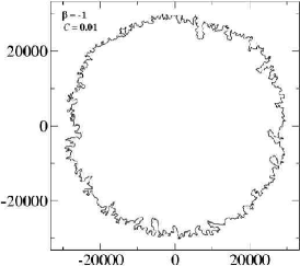
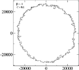
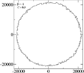
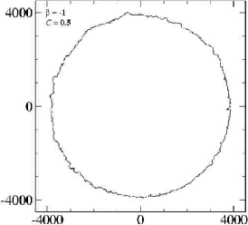
Figure 10: Growth patterns for $\beta=-1$. Panels a-d: ${\cal C}=0.01,0.1,0.3$ and 0.5 respectively.

Therefore our aim is to find a line in the $\beta-{\cal C}$ phase diagram that separates fractal $D<2$ from 2-dimensional growth patterns. That such a line must exist we can convince ourselves by examining the family of growth models that are seen for $\beta=-1$, see Fig. 10. Obviously these are 2-dimensional. The family of growth patterns obtained for $\beta=0$ were shown in Fig. 4, and as we said above, there must be a cross over 2-dimensional patterns in this family. Going up to $\beta=1$ we show the growth patterns in Fig. 11.

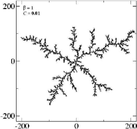
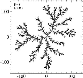
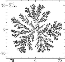
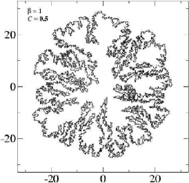
Figure 11: Growth patterns for $\beta=1$. Panels a-d: ${\cal C}=0.01,0.1,0.3$ and 0.5 respectively.

In this case the images indicate that for the lower values of ${\cal C}$ the growth patterns are fractal, whereas for higher values of ${\cal C}$ they become 2-dimensional. Thus the line of separation that we seek in the $\beta-{\cal C}$ phase diagram appears to cut the $\beta=1$ line. Finally, in Fig. 12 we present the family of growth patterns obtained for $\beta=2$.

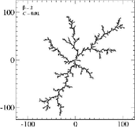
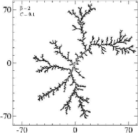
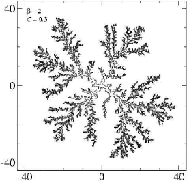
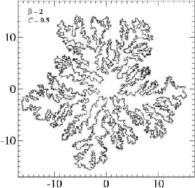
Figure 12: Growth patterns for $\beta=2$. Panels a-d: ${\cal C}=0.01,0.1,0.3$ and 0.5 respectively.

It appears that the transition line intersects also the $\beta=2$ line.

All the patterns exhibited in Figs. 4, 10-12 are grown with a fixed size $\lambda_{0}$. Consequently, for $\beta>0$ the actual mean size of the bumps in the physical space decreases as the cluster grows, while it increases for $\beta<0$. This may lead to worries, i.e. that for $\beta>0$ the growth arrests and that for $\beta<0$ the increase in the size of the bumps leads to coverage of fjords, such that the 2-dimensional patterns shown in Fig. 10 would be an artifact. To disperse these worries we have considered alternative growth algorithms with varying the size of $\lambda_{0}$. The first such algorithm is obtained by requiring that the total area covered in each layer of growth is constant, i.e.

$$\sum_{k=1}^{p}\lambda_{n+k}|{\Phi^{{}^{\prime}(n)}}(e^{i\theta_{n+k}})|^{2}$$

$$= \lambda_{0}(n)\sum_{k=1}^{p}|{\Phi^{{}^{\prime}(n)}}(e^{i\theta_{n+k}})|^{-\beta}={\rm C}\ .$$ (41)

Note that for constant coverage ${\cal C}$ this rule coincides with fixed values of $\lambda_{0}$ for $\beta=2$ (cf. Eq.(11)). In the second algorithm we choose the maximal size of the bump in the physical plane to be constant from layer to layer:

$$\lambda_{0}(n)~{}\max_{k=1}^{p}\{|{\Phi^{{}^{\prime}(n)}}(e^{i\theta_{n+k}})|^{-\beta}\}={\rm C}\ .$$ (42)

This rule coincides with fixed values of $\lambda_{0}$ for $\beta=0$. We found that in all cases the patterns shown above remain invariant to the change of the algorithms. Thus we submit that the figures shown can be fully trusted.

To find the line that separates fractal from 2-dimensional patterns we estimate the dimensions directly from log-log plots of $F^{(n)}$ vs. $S$. We have seen above that such estimates are lower bounds to the actual asymptotic dimension. As these logarithmic plots are invariably concave, we can use the slope at the largest values of area available as a measure for the lower bound on the dimension. In Fig. 13 we show the three lines obtained by searching, for a given value of ${\cal C}$, the value of $\beta$ for which for the first time the dimension estimated from $F^{(n)}$ vs. $S$ crosses the value $D=1.90$ (upper curve), $D=1.95$ (middle line) and $D=1.99$ (lower curve). We propose that the last two lines may very well be already beyond the true line that separates fractal from $D=2$ asymptotic dimension. From the discussion of Sect. IV A we cannot even exclude the possibility that the transition line obfuscates the $\beta=0$ line. All the region below the lower line is almost surely representing patterns of $D=2$, but we strongly believe that this is the case also for the middle line. The lines were obtained by finding, as explained, the values of $\beta$ yielding D=1.90, 1.95 and 1.99 respectively, and then fitting to the points a quadratic function. Next we extrapolated the three fits to values of ${\cal C}$ that are not readily available in our algorithm. The three fit lines intersect the $\beta=2$ line at ${\cal C}=0.73$, 0.78 and ${\cal C}=0.79$ respectively. We thus propose that the value ${\cal C}=1$ for $\beta=2$ is comfortably within the region of 2-dimensional patterns in this phase diagram.

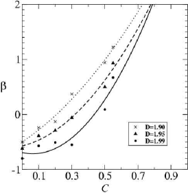
Figure 13: The phase diagram in the $\beta-{\cal C}$ plane. The data points in crosses, triangles and circles represent values of $\beta$ and ${\cal C}$ for which the radius-area relationship predicts $D=1.90$, $D=1.95$ and $D=1.99$ respectively. The lines are quadratic fits. We propose that the region below the lines represents 2-dimensional growth patterns, and see text for details.

VI Conclusions

We have presented a careful numerical study of a 2-parameter model of growth patterns that generalizes and interpolates between Diffusion Limited Aggregation and Laplacian Growth Patterns. The model gives rise to a rich plethora of growth patterns, with fractal dimensions that depend on the values of the parameters $\beta$ and ${\cal C}$. For $\beta=0$ and ${\cal C}=0$ we obtain DLA. Laplacian Growth patterns have $\beta=2$ and ${\cal C}=1$, but we cannot probe the value ${\cal C}=1$ within our algorithm. Since our aim, in part, is to demonstrate that Laplacian Growth patterns are not fractal, we resorted to examining the phase diagram $\beta-{\cal C}$. We established, on the basis of scaling arguments, simulations and visual observations, that this phase diagram contains a line of transition between fractal and 2-dimensional growth patterns. We have estimated the position of this line, and demonstrated that Laplacian Growth patterns belong safely in the region of 2-dimensional growth patterns.

One should point out that the statement that Laplacian Growth are 2-dimensional does not mean that it is a growing disk. To the eye the patterns can look fractal, and in fact radius-area log-log plots might initially even indicate that the dimension is low, and maybe of the order of the dimension of DLA. Deep fjords may exist in the structure. The relevant question is whether the growing branches of the structure contain substance (area) and whether this area is growing relatively with the growth of the pattern. The growth pattern shown in Fig. 11 panel d is a case in point. It looks fractal to the naked eye, but careful examination shows that the branches have area. Thus one needs to decide whether this area is due to some ultraviolet cutoff length, or does it grow systematically beyond what is expected on the basis of the existence of such a cutoff.

Before closing we reiterate that our demonstration that Laplacian Growth patterns are 2-dimensional is not direct. We cannot, within our algorithm, grow ${\cal C}=1$ patterns. We therefore leave this at the moment as a conjecture. It remains a theoretical challenge to show that this conjecture is indeed provable by direct mathematical analysis. We also leave for future work the question whether the $\beta=0$ line represents 2-dimensional growth patterns for all ${\cal C}>0$. Finally we propose that future work may make use of the fractal patterns along the line ${\cal C}=0$, $\beta>0$ for further fundamental studies of DLA and related phenomena.

- (1) F. Barra, B. Davidovitch, A. Leverman and I. Procaccia, Phys. Rev. Lett. 87, 134501 (2001)
- (2) F. Barra, B. Davidovitch and I. Procaccia, “Iterated Conformal Dynamics and Laplacian Growth”, Phys. Rev. E., submitted. Also: cond-mat/0105608
- (3) T.A. Witten and L.M. Sander, Phys. Rev. Lett, 47, 1400 (1981).
- (4) P.G. Saffman and G.I. Taylor, Proc. Roy. Soc. London Series A, 245,312 (1958).
- (5) B. Shraiman and D. Bensimon, Phys.Rev. A30, 2840 (1984); S.D. Howison, J. Fluid Mech. 167, 439 (1986).
- (6) B. Davidovitch, A. Levermann, I. Procaccia, Phys. Rev. E, 62 R5919.
- (7) D. Bensimon, L.P. Kadanoff, S. Liang, B.I. Shraiman and C. Tang, Rev. Mod. Phys. 58, 977 (1986); S. Tanveer, Phil. Trans. R. Soc. Lond. A343, 155 (1993) and references therein.
- (8) L. Paterson, Phys. Rev. Lett. 52, 1621 (1984); L.M. Sander, Nature 322, 789 (1986); J. Nittmann and H.E. Stanley, Nature 321, 663 (1986); H.E. Stanley, in “Fractals and disordered systems”, A. Bunde and S. Havlin (Eds.), Springer-Verlag (1991).
- (9) M.B. Hastings and L.S. Levitov, Physica D 116, 244 (1998).
- (10) B. Davidovitch, H.G.E. Hentschel, Z. Olami, I.Procaccia, L.M. Sander, and E. Somfai, Phys. Rev. E, 59 1368 (1999).
- (11) M. G. Stepanov and L. S. Levitov arXiv:cond-mat/0005456
- (12) H.G.E. Hentschel and I. Procaccia, Physica D8, 435 (1983).
- (13) T.C. Halsey, P. Meakin and I. Procaccia, Phys. Rev. Lett. 56, 854 (1986).
- (14) T.C. Halsey, M.H. Jensen, I. Procaccia, L.P. Kadanoff and B.I. Shraiman, Phys.Rev.A 33, 1141 (1986).
- (15) T.C. Halsey, Phys. Rev. Lett. 72, 1228 (1994).
- (16) P. Grassberger and I. Procaccia, Phys.Rev.Lett. 50, 346 (1983).