A Zero-Temperature Study of Vortex Mobility in
Two-Dimensional Vortex Glass Models

Abstract

Three different vortex glass models are studied by examining the energy barrier against vortex motion across the system. In the two-dimensional gauge glass this energy barrier is found to increase logarithmically with system size which is interpreted as evidence for a low-temperature phase with zero resistivity. Associated with the large energy barriers is a breaking of ergodicity which explains why the well established results from equilibrium studies could fail. The behavior of the more realistic random pinning model is however different with decreasing energy barriers a no finite critical temperature.

The effect of disorder on the behavior of type-II superconductors in magnetic fields is a subject of enormous interest both theoretically and experimentally. Much discussion has the last few years focused on the possibility of a stable vortex glass phase Fisher et al. (1991a) and some recent papers find evidence from simulations for the existence of such a phase in three dimensions Olson and Young (2000); Kawamura (2000); Vestergren et al. (2001). The necessary ingredients of a vortex glass model is, however, still an open question Huse and Seung (1190); Kawamura (2000) and recent results actually suggest that two of the popular models, the gauge glass Olson and Young (2000) and the random pinning model Vestergren et al. (2001), belong to different universality classes.

In two dimensions, which is the focus of the present Letter, the different vortex glass models are commonly believed to behave similarly. One of these is the gauge glass for which equilibrium Nishimori (1994); Fisher et al. (1991b); Gingras (1992); Kosterlitz and Akino (1998) analyses show no transition. In the present paper we approach this model by examining the low-temperature properties of a vortex hopping dynamics. The possibility we explore is that ergodicity breaking might lead to different conclusions when considering dynamics as compared to equilibrium, and we actually find results that strongly suggest a finite-temperature transition. Interestingly, the behavior of the random pinning model is qualitatively different and this points to rich and unexpected behavior of the vortex glass models even in two dimensions.

Results in statistical physics often rely on an assumption of ergodicity. Only if this assumption is valid it is permissible to draw conclusions regarding the physically relevant time-averages from the ensemble averages Binder and Young (1986). Generally speaking this assumption is expected to be valid for models with a smooth energy landscape, whereas an energy landscape with valleys separated by huge energy barriers, could give rise to a breaking of ergodicity. The concept ergodicity breaking presupposes some kind of dynamics and in the present Letter we examine a vortex hopping dynamics where one vortex moves one lattice constant at a time. This is the kind of dynamics that is typically used for the study of dynamical properties in vortex glass models Hyman et al. (1995); Li (1992); Kim (2000).

The possibility of ergodicity breaking means that the standard arguments for the absence of a phase transition could fail and this applies both to the rigorous analytical argument by Nishimori Nishimori (1994) and the vanishing of the zero-temperature domain wall energy with increasing system size Fisher et al. (1991b); Gingras (1992); Kosterlitz and Akino (1998). The dynamical studies should, however, still be reliable, but they arrive at conflicting conclusions. Whereas some have reported evidence for a zero temperature transition Hyman et al. (1995) others are strongly in favor of a transition at a finite temperature Li (1992); Kim (2000). The different conclusions seem to be due to different judgments regarding the reliability of data at rather low temperatures.

In this Letter we present a novel zero-$T$ approach designed to measure the height of the energy barriers in vortex glass models. The quantity in focus is the energy barrier against phase slips (defined more precisely below). Beside probing the possibility of ergodicity breaking this quantity is physically relevant since the resistivity in dynamical simulations is inversely proportional to the time between phase slips. A phase slip energy barrier that diverges as $L\rightarrow\infty$ would suggest both breaking of ergodicity and a vanishing resistivity (= immobile vortices) which in turn implies a superconducting low-temperature phase Kim et al. (1999).

To determine the phase slip energy barrier we start in the ground state and perform an exhaustive search of all relevant local moves, in the vortex representation. Considering the huge phase space of these models this could seem like an impossible task and the only reason why it is at all feasible is that it is sufficient to focus on some relatively few states with rather low energy. Our main result is that the phase slip energy, $V_{L}$, in the gauge glass model grows logarithmically with system size, a finding that we interpret as evidence for the existence of a superconducting low-temperature phase.

The Hamiltonian for the random gauge XY model is

$$H=\sum_{\langle ij\rangle}U\left(\theta_{i}-\theta_{j}-A_{ij}-\frac{1}{L}{\bf r}_{ij}\cdot{\bf\Delta}\right),$$ (1)

where $\theta_{i}$ is the phase at lattice point $i$ on a square lattice of size $L\times L$ (where $L$ is in units of the lattice constant), the sum is over nearest neighbors, and $A_{ij}$ is a randomly chosen vector potential in the interval $[-r\pi,r\pi)$, where $r$ is the disorder strength. The gauge glass model corresponds to the case $r=1$. In the above Hamiltonian we also include the twist variable ${\bf\Delta}=(\Delta_{x},\Delta_{y})$ FTBC to allow for phase slips. The unit vector ${\bf r}_{ij}$ picks $\Delta_{x}$ or $\Delta_{y}$ depending on the direction of the link $ij$.

The spin interaction is often taken to be a cosines function, but to be able to take advantage of the direct relation to the vortex representation we have instead chosen $U(\phi)=J\phi^{2}/2$. With the frustration given by

$$f_{\bf r}=\frac{1}{2\pi}\nabla\times{\bf A}_{\bf r},$$

and fluctuating twists FTBC the vortex Hamiltonian becomes

$$H^{\rm v}=-\frac{1}{2}\sum_{{\bf r},{\bf r}^{\prime}}(q_{\bf r}+f_{\bf r})G({\bf r}-{\bf r}^{\prime})(q_{{\bf r}^{\prime}}+f_{{\bf r}^{\prime}})$$ (2)

where the $q_{\bf r}$ are unit charges, the factor $1/2$ compensates for the double counting, and $G({\bf r})$ is the lattice Green’s function

$$G({\bf r})=\left(\frac{2\pi}{L}\right)^{2}\sum_{{\bf k}\neq 0}\frac{e^{i{\bf k}\cdot{\bf r}}-1}{2\cos k_{x}+2\cos k_{y}-4}.$$

For the discussion of the phase slip energy barrier we start by considering this quantity in the pure 2D XY model. The ground state is trivially given by $q_{\bf r}=0$ for all ${\bf r}$. To consider vortex transport we create a vortex pair with a negative vortex at the origin and a positive at $(1,0)$, and then move the positive one to $(2,0)$, $(3,0)$,…$(L,0)$. The twist variable $\Delta_{y}$ will change proportionally to make the current in the $y$-direction vanish. Since $(L,0)$ in a system with periodic boundary conditions is the same as the origin we are then back again in the ground state but with the twist variable $\Delta_{y}=-2\pi$. (We use the term phase slip for this kind of process even in the vortex representation.) By these steps we have transported unit vorticity across the system. In this simple case the energy for a configuration with the positive vortex at $(x,0)$ is given by the lattice Green’s function, $G(x,0)$, and the phase slip energy barrier for the pure 2D XY model is the value of this energy at the largest separation, $V_{L}=G(L/2,0)$.

For the following we note that each elementary move may be described by a position ${\bf r}$ and a unit dipole vector ${\bf p}$:

$$\begin{array}[]{rcll}q_{\bf r}-1&\rightarrow&q_{\bf r},&\mbox{put a $-1$ vortex at ${\bf r}$},\\ q_{{\bf r}+{\bf p}}+1&\rightarrow&q_{{\bf r}+{\bf p}},&\mbox{put a $+1$ vortex at ${\bf r}+{\bf p}$}.\end{array}$$

To keep track of the transport of vorticity we introduce the polarization ${\bf P}$. An elementary move always changes the polarization, ${\bf P}+{\bf p}\rightarrow{\bf P}$. The vorticity transport discussed above starts in the ground state and ends in the same configuration but with $\Delta P=(L,0)$. The polarization therefore contains some memory of the steps taken and may be used to examine the phase slip.

For the gauge glass model the sequence of elementary moves that corresponds to the lowest possible energy barrier is in general much more complex than in the pure XY model. To illustrate this point we show in Fig. 1 such a sequence of moves for a certain disorder realization in a $4\times 4$ system. In this case six steps are needed to transport vorticity across the system and return back to the ground state. We now describe the method used to find such complex paths.

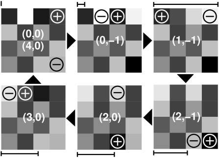
Figure 1: Illustration of a sequence of elementary moves for a realization of a $4\times 4$-system, corresponding to transport of vorticity across the system, $\Delta{\bf P}=(4,0)$. The upper left corner is the ground state. Charge is symbolized by the shading of the squares, black represents $-0.67$, white represents $+0.72$, and intermediate charges are proportionally grey. The digits show the polarization relative to the ground state. The charge symbols represent the dipole excited in the next step. The bar next to the square shows the energy of each configuration relative to the ground state.

We first search for the ground state by applying the standard spin quench algorithm Walker and Walstedt (1980) a large number of times. The lowest energy state is taken to be the true ground state when it has been found $N_{\rm rep}=10$ times. No change was found in the results when we instead used $N_{\rm rep}=100$ for a set of $10^{4}$ disorder configurations with $L=4$. We then use an algorithm that is analogous to the filling of a (energy) landscape with a liquid rising from a source at the lowest position. At each time step it is the lowest level accessible by the liquid that is invaded. The disorder configurations give rise to different periodic energy landscapes in polarization space, and the liquid is made to rise until there is a connection between these periodic copies. The landscape picture is, however, a great over-simplification. For each value of the polarization there is a large number of possible configurations with different energy. The true picture is therefore more of a plumber’s nightmare with a large network of pipes criss-crossing the polarization space but the intuitive picture still holds. With an algorithm that slowly increases the level one is guaranteed that the first connection found is the lowest possible.

In the computer, the algorithm consists of repeating the following steps:

1. Generate $4L^{2}$ configurations by applying the $4L^{2}$ possible dipole excitations to the current configuration.

2. Calculate the energy of each such configuration and put them in a sorted list, lowest energy first, together with their polarization relative to the ground state.

3. Take the first (lowest energy) configuration from this list to be the new current configuration.

4. If this configuration has already been encountered, but with a different polarization such that $\Delta{\bf P}=(\pm L,0)$ then we are done. Otherwise, go to step 1.

To make this algorithm work one also needs a list of already used configurations. In step 1 the current configuration is added to that list and in step 4 each configuration is compared to the list. The main output is the phase slip energy barrier which equals the highest energy used in the algorithm. The data below are obtained by averaging the energy barrier from 3000 to $2\times 10^{5}$ disorder configurations. Much as expected, the number of iterations, $N$, of the above algorithm grows rapidly with $L$, $N\approx 0.5\exp L$. In our simulations the spin quench algorithm that is used to find the ground state is however more time consuming than the determination of the energy barrier.

Figure 2 shows $V_{L}$ versus $L$ for several different values of $r$. We first focus on the results for $r=1$, the usual gauge glass model, shown by solid diamonds in panel (a). By plotting the data with log scale on the $x$ axis it is found that the points with $L\geq 3$ to an excellent approximation fall on a straight line with a positive slope. We consider this to be strong evidence for an energy barrier that diverges with increasing lattice size and thereby also evidence for the existence of a low-temperature phase with immobile vortices. As shown in the figure the scaling holds down to $L=3$. This is the same size as in the examinations of the domain wall energy in the gauge glass Kosterlitz and Akino (1998) and it therefore seems likely that the logarithmic increase in Fig. 2 is the true behavior at large $L$. As further support for this belief we note that the logarithmic size-dependence is not a foreign behavior, but is rather built into the model at the outset through the logarithmic length-dependence in the vortex interaction.

Figure 2: Size dependence of the phase slip energy $V_{L}$ for the random gauge XY model. The result for the gauge glass ($r=1$) are shown by the solid diamonds in panel (a) whereas the results for the ordinary 2D XY model ($r=0$) are shown by crosses in panel (b). We always find $V_{L}\sim\log L$ which suggests diverging energy barriers against vortex motion and a superconducting low-temperature phase. Panel (c) shows the slope of the lines in (b). There are error bars corresponding to one standard deviation for all the data points, but most of them are far too small to be visible.

For weaker disorder, $r<1$, the general feature is the same with $V_{L}\sim\log L$. Considering the change in behavior as $r$ decreases we find that $V_{L}$ initially changes very slowly. The values of $V_{L}$ for $r=0.9$ and 0.8 (not shown) are almost identical to the ones for $r=1$. For an analysis of the data for $r\leq 0.7$ we fit $V_{L}=a(r)+b(r)\ln L$, shown by solid lines. When $r$ is reduced below $\approx 0.8$, $a(r)$ slowly increases but the slope $b(r)$ at first remains unchanged, Fig. 2c. The slope actually to a good approximation remains constant down to $r=0.5$ where it starts to increase and finally approaches $b(0)=2\pi$ of the pure 2D XY model. We believe that the behavior of the slope $b$ shown in panel (c) is related to the finding Kosterlitz and Simkin (1997); Maucourt and Grempel (1997) of a phase with quasi long range order (without ergodicity breaking) for $r<r_{c}\approx 0.37$. Figure 2c is also very similar to the phase diagram for the same model recently obtained on the basis of Monte Carlo simulations Holme et al. .

Since the gauge glass model is an often used model of a disordered superconductor in an applied magnetic field, the above result would quite surprisingly seem to suggest the existence of a dissipation-free low temperature phase in disordered thin superconducting films. To examine this question in more detail we have also studied the phase slip energy in the random pinning model introduced in Ref. Hyman et al. (1995), which is meant to be a more realistic model of a disordered superconductor in an applied magnetic field. The difference is that the random pinning model has a constant non-zero magnetic field at each plaquette whereas the random gauge XY model instead is a superconductor with random fields that sum up to zero. The Hamiltonian for the random pinning model is

$$H_{\rm rp}=-\frac{1}{2}\sum_{{\bf r},{\bf r}^{\prime}}(q_{\bf r}-f)G({\bf r}-{\bf r}^{\prime})(q_{{\bf r}^{\prime}}-f)-\sum_{\bf r}v_{\bf r}q_{\bf r}^{2}.$$ (3)

The frustration (magnetic field) is here homogeneous and the disorder is instead included through the pinning potential $v_{\bf r}$. We follow Ref. Hyman et al. (1995) and let $v_{\bf r}$ be a random variable uniformly distributed between $-\pi$ and $\pi$, and restrict the possible values for the vorticity to $q_{\bf r}=-1,0,1$.

Figure 3: Size-dependence of $V_{L}$ for the random pinning model with three different values for the frustration. The energy barrier decreases with increasing $L$.

Figure 3 shows the size dependence of $V_{L}$ for the random pinning model with $f=1/3$, $1/4$, and $1/9$. Due to the requirement that $fL^{2}$ has to be an integer it is only possible to get data for a few lattice sizes for each value of $f$. The behavior is here markedly different from what we found in the gauge glass; $V_{L}$ decreases with increasing lattice size and we therefore conclude that the phase slip energy barrier vanishes in the thermodynamic limit. The results are therefore very different from Ref. Hyman et al. (1995) where it was concluded from a scaling analysis of the $I$-$V$ characteristics that the gauge glass model and the random pinning model do belong to the same universality class. Interestingly, recent simulations strongly suggest that the three-dimensional versions of these two models belong to different universality classes Olson and Young (2000); Vestergren et al. (2001).

We also shortly mention our results for a generalized XY spin glass, which is given by the same Hamiltonian as the gauge glass but with only two possible values for the vector potential, $A_{ij}=0$, $\pi$. Let $s$ denote the fraction of links with $A_{ij}=\pi$. Due to the chiral symmetry every ground state has a chiral mirror image $q_{\bf r}\mapsto-q_{\bf r}$ that is also a ground state. We may therefore define a chiral energy barrier $V_{L}^{c}$, as the energy barrier that has to be climbed to reach the chirally mirrored ground state.

Figure 4: The energy barrier for $2\pi$ phase slip $V_{L}$ (a) and chiral mirroring $V_{L}^{c}$ (b) for the generalized $2\pi$ XY spin glass. For the ordinary XY model ($s=0$) $V_{L}$ is shown in Fig. 2 while $V_{L}^{c}$ would be identically zero.

The phase slip energy $V_{L}$ is shown in Fig. 4a. For $s\geq 0$ $V_{L}$ is independent of size. For $s=0.05$ the data seems to go as $\log L$ suggesting a critical $s_{c}>0.05$, but we cannot exclude the possibility that $V_{L}$ saturates and approaches a constant for $L\geq 5$. The behavior of the chiral energy barrier in Fig. 4b is different, suggesting $V_{L}^{c}\sim\log L$ for all $s>0$ which means that the system at low temperatures and with only local moves is trapped in the part of the configuration space with the given chirality.

To conclude, we have examined the existence of growing energy barriers and thereby a possible breaking of ergodicity in three different 2D vortex glass models. By examining the phase slip energy barrier $V_{L}$ we found different behaviors in these three models. In the gauge glass $V_{L}$ increases logarithmically which we take to suggest the existence of a low-temperature phase with zero resistivity. In the more realistic random pinning model $V_{L}$ instead decreases in accordance with a transition at zero temperature. Yet another behavior is found in the XY spin glass where $V_{L}$ is independent of $L$.

We thank B. J. Kim, P. Minnhagen, and S. Teitel for valuable discussions. This work was supported by the Swedish Natural Science Research Council through Contract No. E 5106-1643/1999.

References

- Fisher et al. (1991a) D. S. Fisher, M. P. A. Fisher, and D. A. Huse, Phys. Rev. B 43, 130 (1991a).
- Kawamura (2000) H. Kawamura, J. Phys. Soc. Jpn. 69, 29 (2000).
- Olson and Young (2000) T. Olson and A. P. Young, Phys. Rev. B 61, 12467 (2000).
- Vestergren et al. (2001) A. Vestergren, J. Lidmar, and M. Wallin (2001), unpublished.
- Huse and Seung (1190) D. A. Huse and H. S. Seung, Phys. Rev. B 42, 1059 (1190).
- Nishimori (1994) H. Nishimori, Physica A 205, 1 (1994).
- Fisher et al. (1991b) M. P. A. Fisher, T. A. Tokuyasu, and A. P. Young, Phys. Rev. Lett. 66, 2931 (1991b).
- Gingras (1992) M. J. P. Gingras, Phys. Rev. B 45, 7547 (1992).
- Kosterlitz and Akino (1998) J. M. Kosterlitz and N. Akino, Phys. Rev. Lett. 81, 4672 (1998).
- Binder and Young (1986) K. Binder and A. P. Young, Rev. Mod. Phys. 58, 801 (1986).
- Hyman et al. (1995) R. A. Hyman, M. Wallin, M. P. A. Fisher, S. M. Girvin, and A. P. Young, Phys. Rev. B 51, 15304 (1995).
- Li (1992) Y.-H. Li, Phys. Rev. Lett. 69, 1819 (1992).
- Kim (2000) B. J. Kim, Phys. Rev. B 62, 644 (2000).
- Kim et al. (1999) B. J. Kim, P. Minnhagen, and P. Olsson, Phys. Rev. B 59, 11506 (1999).
- (15) A. Vallat and H. Beck, Phys. Rev. B 50, 4015 (1994); P. Olsson, Phys. Rev. B 46, 14598 (1992); P. Olsson, Phys. Rev. B 52, 4511 (1995); B. J. Kim, P. Minnhagen, and P. Olsson, Phys. Rev. B 59, 11506 (1999).
- Walker and Walstedt (1980) L. R. Walker and R. E. Walstedt, Phys. Rev. B 22, 3816 (1980).
- Kosterlitz and Simkin (1997) J. M. Kosterlitz and M. V. Simkin, Phys. Rev. Lett. 79, 1098 (1997).
- Maucourt and Grempel (1997) J. Maucourt and D. R. Grempel, Phys. Rev. B 56, 2572 (1997).
- (19) P. Holme, B. J. Kim, and P. Minnhagen.