Voltage-tunable singlet-triplet transition in lateral quantum dots

Abstract

Results of calculations and high source-drain transport measurements are presented which demonstrate voltage-tunable entanglement of electron pairs in lateral quantum dots. At a fixed magnetic field, the application of a judiciously-chosen gate voltage alters the ground-state of an electron pair from an entagled spin singlet to a spin triplet.

I Introduction

Proposals for spin-based quantum computation in a solid-state environmentBarenco et al. (1995); Brum and Hawrylak (1997); Loss and DiVincenzo (1998); Kane (1998); Vrijen et al. (2000) require efficient techniques for manipulating the entanglement of coupled qubits. In this paper, we demonstrate theoretically and verify experimentally that ground-state entaglement can be induced solely by applying a potential to the gates. This is possible because the gate voltage controls not only the chemical potential of the dot, but the shape of the confining potential as well. Consequently, the gate voltage can induce transitions in the dot containing a well-defined, constant number of particles.

Early far-infrared measurements on arrays of few-electron dots,Sikorski and Merkt (1989); Meurer et al. (1992) and transport through single devicesSu et al. (1992) were focused on the tunability of the electron number and, although transitions were observed, it was difficult to assign, for example, quantum numbers to these transitions. Later experiments using single-particle capacitanceAshoori et al. (1993) and magneto-tunnelingSchmidt et al. (1995) spectroscopy focused on the evolution of the ground states as a function of magnetic field and were able to distinguish features consistent with the two-electron singlet-triplet transition. High source-drain tunneling spectroscopy probes the excited states as well as the ground state and therefore the singlet-triplet transition can be more clearly and unambiguously observed. This has already been successfully applied to etched vertical quantum dots with (spin) unpolarized leads.Kouwenhoven et al. (1997); van der Wiel et al. (1998) In the lateral devices employed in the present study, the dot is formed within a 2-dimensional electron gas (2DEG), with the lateral confinement produced electrostatically by voltages applied to gates located above the 2DEG. Recent work employing a novel gate designCiorga et al. (2000) has allowed the electron-number $N$ to be tuned down to a single electron.

There are at least two features unique in the lateral devices. First, since the leads are essentially 2DEG edges, applying a rather weak magnetic field—approximately 0.4 T in practice—is sufficient to produce spin-resolved edges.Sachrajda et al. (2001) Therefore, the tunneling rates into and out of the dots are significantly different for each species of spin. This spin-polarized injection (and detection) allows us to distinguish orbital effects from spin effects in transport measurements.Ciorga et al. (2000); Sachrajda et al. (2001); Ciorga et al. (2001, 2002a) Second, since the confinement potential is formed electrostatically by the various gate voltages, altering the shape—in particular the non-parabolicity—of the quantum dot can be accomplished while keeping the particle number fixed. It is important to note that the familiar singlet-triplet transition is not caused by the difference in Zeeman energy but rather by changes in the orbital part of the wavefunction. In multiple-dot systems, in particular with regards to quantum-dot-based quantum computation,Loss and DiVincenzo (1998) this versatility is of crucial importance. Quantum-state engineering of this sort is clearly observable in the experimental results we present below.

From the theoretical side, numerical analyses of the interacting two-electronWagner et al. (1992); Pfannkuche et al. (1993); Hawrylak (1993a) problem, as well as higher electron numbers,Hawrylak (1993a); Pederiva et al. (2000) demonstrated singlet-triplet transitions in parabolic potentials using either a fixed or an $N$-dependent harmonic frequency. These works focused on magnetic-field-induced transitions. In our experiment, the confining potential is a function of the continuous variables $V_{g}$ (the gate voltages) and the confinement in our particular quantum dots deviate from parabolicity. These features, which are addressed in our theory, allow a spin phase diagram to be constructed in the gate-voltage/magnetic-field plane and clearly indicate how the $N=2$ singlet-triplet transition can be externally engineered at fixed magnetic field. In double-dot systems containing one electron apiece, similar transitions, and for similar reasons, have been theoretically demonstrated in both lateralBurkard et al. (1999); Hu and Sarma (2000) and verticalBurkard et al. (2000) devices. Our theory is applicable to these systems with only a few modifications related to the orbital degrees of freedom—the spin physics are essentially equivalent.

In the Coulomb-blockade regime, transport experiments probe the two-electron system either by adding an electron to the one-electron droplet, or by removing an electron from the three-electron droplet. Each case corresponds to a distinct gate voltage, and in each case the ground and excited states can be probed by high source-drain spectroscopy, which directly reveals the singlet-triplet transition. Our theory and experiment show that, for these two different gate voltages, the transition between the entangled spin singlet $\left|\uparrow\downarrow\right\rangle-\left|\downarrow\uparrow\right\rangle$ and the spin triplet $\left|\downarrow\downarrow\right\rangle$ occurs at two different magnetic fields.

The paper is organized as follows: Section II describes the experimental results, including the demonstration of a gate-voltage-induced singlet-triplet transition. Section III contains a theoretical analysis, culminating in the spin phase diagram of the $N=2$ interacting system in the gate-voltage/magnetic-field plane. Finally, Sec. IV contains a concluding discussion.

II Experimental results

An SEM image of a device similar to the one used in our experiments is shown in Fig. 1.

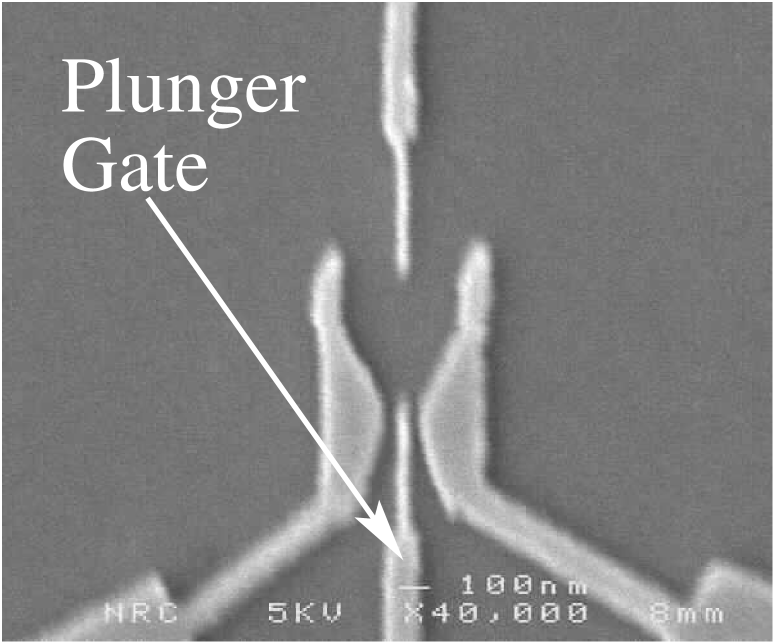
Figure 1: SEM image of the gate geometry forming the quantum dot. This geometry enables a precisely known number of electrons ($N=0,1,2,\ldots,50$) to be trappedCiorga et al. (2000) and produces a quasi-parabolic confinement potential. Sweeping the plunger-gate voltage tunes both the shape and the chemical potential of the quantum dot.

This geometry allows us to controllably tune the number of trapped electrons in the 2DEG—90 nm below the surface—from about fifty down to a single electron.Ciorga et al. (2000) High source-drain transport measurements in the Coulomb-blockade regime were carried out in order to detect both the ground and excited states of the two-electron system. Standard low-power ac measurement techniques were used with a 10 $\mu$V excitation voltage applied across the sample at a frequency of 23 Hz. An additional dc voltage was applied in order to obtain a high source-drain bias. The differential conductance $dI/dV_{\text{sd}}$ is measured directly in such a configuration and the relevant data is shown in Fig. 2 for a source-drain voltage of 350 $\mu$V.

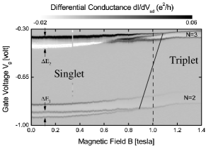
Figure 2: High source-drain transport spectroscopy of the two-electron droplet. The lower set of curves corresponds to fluctuations between $N=1$ and $N=2$, while the upper set corresponds to fluctuations between $N=2$ and $N=3$. Both sets of curves probe the same states of the two-electron droplet (ground plus first excited state) but at different gate voltages. The singlet-triplet transition is seen to occur at two different critical fields. The solid line marks the singlet-triplet ground-state boundary. This boundary can be traversed along the dashed line at $B=1$ T solely by adjusting the (plunger) gate voltage.

In this figure we show the inverted grayscale for the $N=2$ subspace as a function of magnetic field $B$ and plunger gate voltage $V_{g}$. The negative differential conductance, which is also tunable,Ciorga et al. (2002b) is related to the spin-polarized injection of electrons.

For the lowest set of curves in Fig. 2, transport proceeds through the addition and subtraction of a second electron from a one-electron droplet. At the lowest curve, transport is predominately through the ground state of the two-electron droplet (a spin singlet at low fields); beginning at the curve immediately above this one, transport through the first excited state (a spin triplet at low fields) is also allowed. Hence, the exchange constant can be directly obtained experimentally from these curves by suitably calibrating the parameters relating gate voltage to energy. The singlet-triplet transition is clearly seen (cf. etched vertical dotsKouwenhoven et al. (1997); van der Wiel et al. (1998)) at a field of $B_{c1}\approx 0.92$ T. The upper set of curves corresponds to adding and removing a third electron from the two-electron system. After the third electron has left the dot, the resulting two-electron droplet can either be in the ground state or an excited state. (Transport through the ground state is the topmost curve.) Therefore, it should be possible to extract the same exchange constant from these curves as described above for the lower set of curves. Indeed, the singlet-triplet transition is again clearly seen, but now occurs at a field of $B_{c2}\approx 1.1$ T. The singlet-triplet gaps for the two different cases are shown in Fig. 3—the central experimental result of this work.

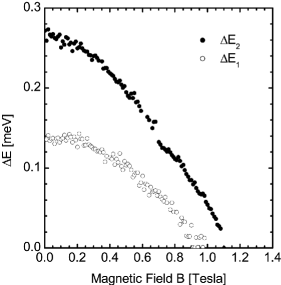
Figure 3: Singlet-triplet gap $J=\Delta E$ as a function of magnetic field for two different gate voltages, as described in the text. $\Delta E_{1}$ and $\Delta E_{2}$ are also denoted in Fig. 2.

Two important conclusions can be drawn from Fig. 3, each of which is verified in the subsequent sections. First, because the gaps do not close linearly, the confinement potential cannot be parabolic. Second, because the two curves do not fall on each other, the actual shape of the dot must be different for the two curves. This change can only be due to the gate voltage, and it therefore follows that the gates themselves can be used to tune through the singlet-triplet transition and hence tune the ground-state entanglement of the system. Figure 2 shows how this may be accomplished. The solid line demarcates the boundary between the singlet and triplet ground-state phases. At a fixed field of 1 T (marked on the figure as a dashed line) the ground-state entanglement can be tuned to be either a singlet or a triplet solely by adjusting the gate voltage appropriately.

In the following, we present the theoretical justification of the above statements.

III Theoretical results

We begin this section with a description of the model we shall use throughout the paper. We shall work primarily in the 2D harmonic oscillator (Fock-Darwin) basis, characterized by the two oscillator quantum numbers $m,n=0,1,2,\dots$ and the spin quantum number $\sigma=\pm 1/2$. This is the diagonal basis of 2D electrons (taken to lie in the $x$-$y$ plane) with charge $-e$ and effective mass $m^{*}$, moving in a uniform magnetic field $\boldsymbol{B}=(0,0,B)$ oriented perpendicular to the 2DEG plane, and with a parabolic confinement potential $V_{\text{par}}=m^{*}\omega_{0}^{2}(x^{2}+y^{2})/2$. The single-particle energy levels are given by the familiar Zeeman-split Fock-Darwin spectrum:Fock (1928); Darwin (1930); Jacak et al. (1997)

$$\varepsilon_{mn\sigma}=\Omega_{+}\left(n+\frac{1}{2}\right)+\Omega_{-}\left(m+\frac{1}{2}\right)+g\mu_{B}B\sigma.$$ (1)

The first two terms in this equation are the oscillator energies, with $\Omega_{\pm}=(\sqrt{\omega_{c}^{2}+(2\omega_{0})^{2}}\pm\omega_{c})/2$, $\omega_{c}=eB/(m^{*}c)$ denoting the cyclotron frequency, and $\omega_{0}$ the parabolic confinement frequency. The final term is the Zeeman energy, where $g\mu_{B}B\approx 0.012\hbar\omega_{c}$ in GaAs.

Neglecting environmental influences, the Hamiltonian of an isolated quantum dot can be written in the Fock-Darwin basisJacak et al. (1997) as

$$H=\sum_{i,\sigma}\varepsilon_{i\sigma}c^{\dagger}_{i\sigma}c_{i\sigma}+\gamma\sum_{i,j,\sigma}h_{ij}c^{\dagger}_{i\sigma}c_{j\sigma}\\ \mbox{}+\alpha\!\sum_{\begin{subarray}{c}i,j,k,l,\\ \sigma,\sigma^{\prime}\end{subarray}}V_{ij}^{k\ell}c^{\dagger}_{i\sigma}c^{\dagger}_{j\sigma^{\prime}}c_{k\sigma^{\prime}}c_{\ell\sigma},$$ (2)

where the Latin indices $i,j,k,l$ are a composite denoting the two oscillator quantum numbers $m$ and $n$. The operator $c^{\dagger}_{i\sigma}\rightarrow c^{\dagger}_{mn\sigma}$ creates a particle in the state $|mn\sigma\rangle$ with the $z$-component of angular momentum $(m-n)$, and $c_{i\sigma}$ is the conjugate annihilation operator. Unless otherwise noted, all energies are expressed in units of the effective Rydberg $\text{Ry}=m^{*}e^{4}/(2\hbar^{2})$ ($\approx 5.9$ meV in GaAs), and all lengths in units of the effective Bohr radius $a_{0}=\hbar^{2}/(m^{*}e^{2})$ ($\approx 9.8$ nm in GaAs).

The diagonal one-body term—the first term in Eq. (2)—is just the Fock-Darwin energy coming from parabolic confinement; $\varepsilon_{i\sigma}\rightarrow\varepsilon_{mn\sigma}$ is given in Eq. (1). We consider the total confinement to be composed of a parabolic piece plus a non-parabolic piece; the parabolic piece, along with the kinetic energy, is incorporated into the diagonal term; the non-parabolic piece is represented by the off-diagonal one-body term—the second term in Eq. (2)—whose overall strength is governed by the dimensionless parameter $\gamma$. This term directly affects the single-particle spectrum, and also significantly alters the singlet-triplet transition in the two-electron droplet. We discuss this term in detail in Sec. III.2.

Finally, the two-body term in Eq. (2) represents interactions, where the matrix element $V_{ij}^{kl}\rightarrow\langle m_{1},n_{1};m_{2},n_{2}|e^{2}/(\epsilon|\vec{r}_{1}-\vec{r}_{2}|)|m_{3},n_{3};m_{4},n_{4}\rangle$ is the full Coulomb interaction in the 2D harmonic oscillator basis ($\epsilon$ is the dielectric constant); an exact expression is given by Hawrylak (1993b)

$$V_{ij}^{kl}\rightarrow\frac{E_{0}}{\sqrt{2\pi}}\,\delta_{R_{L},R_{R}}\frac{(-1)^{n_{2}+m_{2}+n_{3}+m_{3}}}{\sqrt{n_{1}!m_{1}!n_{2}!m_{2}!n_{3}!m_{3}!n_{4}!m_{4}!}}\sum_{k_{1}=0}^{\text{min}(m_{1},m_{4})}k_{1}!\begin{pmatrix}m_{1}\\ k_{1}\end{pmatrix}\begin{pmatrix}m_{4}\\ k_{1}\end{pmatrix}\sum_{k_{2}=0}^{\text{min}(n_{1},n_{4})}k_{2}!\begin{pmatrix}n_{1}\\ k_{2}\end{pmatrix}\begin{pmatrix}n_{4}\\ k_{2}\end{pmatrix}\\ \mbox{}\times\sum_{k_{3}=0}^{\text{min}(m_{2},m_{3})}k_{1}!\begin{pmatrix}m_{2}\\ k_{3}\end{pmatrix}\begin{pmatrix}m_{3}\\ k_{3}\end{pmatrix}\sum_{k_{4}=0}^{\text{min}(n_{2},n_{3})}k_{2}!\begin{pmatrix}n_{2}\\ k_{4}\end{pmatrix}\begin{pmatrix}n_{3}\\ k_{4}\end{pmatrix}\left(\frac{-1}{2}\right)^{k}\Gamma\left(k+\frac{1}{2}\right).$$ (3)

The energy scale of the Coulomb interaction is set by $E_{0}\equiv\sqrt{\pi/2}\,e^{2}/(\epsilon\ell_{0})$ where the hybrid length $\ell_{0}^{2}=\hbar c/(eB\sqrt{1+4\omega_{0}^{2}/\omega_{c}^{2}})$. $E_{0}$ is the sum of all exchange energies in the lowest Landau level, i.e., $\sum_{m=0}^{\infty}\langle m,0;0,0|e^{2}/(\epsilon|\vec{r}_{1}-\vec{r}_{2}|)|m,0;0,0\rangle=E_{0}$, and, additionally, $\langle 0,0;0,0|e^{2}/(\epsilon|\vec{r}_{1}-\vec{r}_{2}|)|0,0;0,0\rangle=E_{0}/\sqrt{2}$. The Coulomb interaction conserves angular momentum $R\equiv\sum_{i}(m_{i}-n_{i})$. This is enforced in Eq. (3) by the Kronecker delta function: $R_{L}=(m_{1}-n_{1})+(m_{2}-n_{2})$, $R_{R}=(m_{3}-n_{3})+(m_{4}-n_{4})$. Also in Eq. (3), $k=(m_{1}+m_{2}+n_{3}+n_{4})-(k_{1}+k_{2}+k_{3}+k_{4}),\ \text{and}\ \Gamma(k+1/2)$ is the Gamma function.

The dimensionless parameter $\alpha$ in Eq. (2) controls the strength of the Coulomb interaction, with $\alpha=1$ representing “bare” Coulomb interactions. At long length scales, screening effects from the nearby metallic gates and leads decrease the strength of the Coulomb interaction. At short length scales, the finite width of the 2DEG layer also decreases the strength of interactions. Since Coulomb interactions are not the primary focus at present, we shall use the parameter $0\leq\alpha\leq 1$ to describe the strength of Coulomb interactions, rather than considering a more sophisticated functional form.

In order to determine which of the main results are specific to the details of the confinement and which are more general, we shall first consider the usual parabolic confinement, and subsequently investigate the particular deviations from parabolicity present in our device.

III.1 Parabolic confinement

In this section, we consider the case of pure parabolic confinement ($\gamma=0$). We shall see that our central result of voltage-tuned entanglement is already present in this simple case.

III.1.1 Non-interacting electrons

The single-particle problem with parabolic confinement ($\gamma=\alpha=0$) yields the Fock-Darwin spectrum in Eq. (1). This approximation should be most valid for the lowest-energy level of the one-electron droplet; in addition to having no intra-dot Coulomb interactions, the zero-point energy should be smallest for the one-electron droplet. A comparison of the Fock-Darwin spectrum and experiment is shown in Fig. 4.

Figure 4: Comparison of experiment and theory for the one-electron droplet. The data was fit to Eq. (1), with $\omega_{0}$ as a fitting parameter.

The experimental points are the position of current peak as a function of magnetic field for the one-electron droplet. The parabolic confinement frequency $\omega_{0}$ was used as a fitting parameter, with $\omega_{0}=1$ meV being displayed in the figure. Although the data is well-fit for this value, we shall find a rather different situation for the two-electron droplet.

III.1.2 Interacting electrons

When Coulomb interactions are switched on (but with $\gamma=0$ for the moment), $m$ and $n$ are no longer good quantum numbers, but, since circular symmetry is still manifest, the total angular momentum $R$ is indeed conserved, as are total spin $S$ and total $S_{z}$. The Hamiltonian can therefore be diagonalized in each $(R,S,S_{z})$ subspace separately.

We have numerically diagonalized Eq. (2) with $\gamma=0$ according to the following procedure: We work in a fixed $(R,S_{z})$ subspace—alternatively,Wensauer et al. one may work in a fixed $(R,S,S_{z})$ subspace, a particularly useful approach for larger particle numbers—and we use the 2D harmonic oscillator basis, with the Coulomb matrix elements given by Eq. (3). We truncate the infinite-dimensional Hilbert space by introducing a high-energy cutoff $E_{\text{cutoff}}$; For each $N$-particle basis vector $|m_{1}n_{1}\sigma_{1},\ldots,m_{N}n_{N}\sigma_{N}\rangle$, we calculate its ($\alpha=0$) eigenenergy and discard it if this energy is greater than $E_{\text{cutoff}}$. We then numerically diagonalize the resulting finite-dimensional Hamiltonian $\langle m_{N}n_{N}\sigma_{N},\ldots,m_{1}n_{1}\sigma_{1}|H|m_{1}^{\prime}n_{1}^{\prime}\sigma_{1}^{\prime},\ldots,m_{N}^{\prime}n_{N}^{\prime}\sigma_{N}^{\prime}\rangle$ (with finite $\alpha$) to obtain both the eigenstates and the spectrum. We then keep repeating this process with a progressively larger $E_{\text{cutoff}}$ until the eigenvalues converge to a constant value.

For small magnetic fields ($B<5$ T, for $\omega_{0}=1$ meV) and two electrons, convergence is reached rather quickly. For example, for a 112-dimensional Hilbert space, convergence to within 4% has been achieved for the lowest 65 eigenstates for $(N,B,R,S_{z})=(2,0,1,0)$ (this spin value includes both singlet and triplet states), and to within 0.5% for the lowest 49 eigenstates. The eigenvalues for $R=-10$ to 10, $B=0$, and $S_{z}=0$ are shown in Fig. 5.

Figure 5: Eigenvalues of the interacting two-electron droplet with parabolic confinement. The plot is for $B=0$ T, $\omega_{0}=1$ meV, and for singlets and triplets with $S_{z}=0$.

Experimentally, we have seen that the magneto-transport data of the one-electron droplet is very well described by parabolic confinement with a confinement frequency of $\omega_{0}=1$ meV. In the two-electron droplet, where Coulomb interactions are now relevant, the ground-state singlet-triplet transition is experimentally seen to occur at approximately $B_{c}=1$ T. If we assume the confinement frequency remains constant at 1 meV, then $B_{c}=1$ T occurs for $\alpha\approx 0.2$, and thus Coulomb interactions are significantly reduced from their bare value. Alternatively, since the critical field scales with the ratio $\omega_{0}/(\alpha E_{0})$, $\omega_{0}$ may increase, rather that $\alpha$ decrease, to give the same effect. This is shown in Fig. 6, where all curves are for the case $\alpha=1$.

Figure 6: Inset: Lowest-energy singlet $|S,S_{z}\rangle=|0,0\rangle$ (lower curve) and triplet $|1,-1\rangle$ (upper curve) for the two-electron droplet with $\alpha=1$ and $\omega_{0}=1$ meV. The singlet-triplet gap $J$ is indicated. Main plot: Singlet-triplet gap as a function of magnetic field for the two-electron droplet with $\alpha=1$. The upper curve has $\omega_{0}=1.5$ meV and the lower has $\omega_{0}=1$ meV.

The main plot shows the evolution of the singlet-triplet gap $J$ with magnetic field. The lower curve has $\omega_{0}=1$ meV while the upper has $\omega_{0}=1.5$ meV. The inset shows the actual singlet-triplet crossing for $\omega_{0}=1$ meV. This simple model of parabolic confinement with full Coulomb interactions is clearly insufficient to quantitatively reproduce the experimental findings of Fig. 3. The linear closing of the gap in the theory—there are actually very slight deviations from linearity not discernible in Fig. 6—appears to be a feature of Coulomb interactions combined with parabolic confinement. The experimental curves of Fig. 3 are thus an indication that the confinement is non-parabolic.

What this simple theory does capture, is that the critical-field $B_{c}(\omega_{0})$ is controlled by the gate voltage via its influence on the confining frequency $\omega_{0}(V_{g})$ for a fixed particle number $N$. Thus, already at this level, we see how the gate voltage, at fixed uniform magnetic field, can be used to tune through the singlet-triplet transition.

The parabolic-confinement model is insufficient to reproduce both the critical field $B_{c}$ and the zero-field gap $J_{0}=J(B=0)$. Finite-width effects ($\alpha<1$) or an increasing $\omega_{0}$ serve to increase both $B_{c}$ and $J_{0}$. In the following section, we investigate the influence of non-parabolic confinement on the singlet-triplet gap.

III.2 Non-parabolic confinement

The confinement potential produced by the gate geometry shown in Fig. 1 exhibits only approximate circular symmetry and this explicit symmetry breaking can be clearly seen in experiment already at the two-electron level, as shown in Fig. 3. This deviation from parabolicity is included as the second term of our model in Eq. (2), and it is the influence of this term we investigate in this section.

The first problem is to obtain a functional form for the confinement potential. Since the gate voltages are the primary contribution to the confinement potential, the simplest approach is to consider the electrostatic potential in the 2DEG induced by the gate voltages. Defining the $x$-$y$ plane to be the plane of the gates so that the potential $V(\boldsymbol{r},z=0)$ is experimentally given ($\boldsymbol{r}\equiv(x,y)$), an analytic expression can be derivedDavies et al. (1995) for the potential $V(\boldsymbol{r},z)$ at an arbitrary point:

$$V\left(\boldsymbol{r},z\right)=\int\frac{d\boldsymbol{r}^{\prime}}{2\pi}\,|z|\,\frac{V(\boldsymbol{r}^{\prime},0)}{\left(z^{2}+\left|\boldsymbol{r}-\boldsymbol{r}^{\prime}\right|^{2}\right)^{3/2}}.$$ (4)

This equation yields the correct $z\rightarrow 0$ limit, as well as $\partial V/\partial z\rightarrow 0$ for $|z|\rightarrow\infty$. The integration, performed at each point $\boldsymbol{r}$ in the 2DEG plane ($z=90\ \text{nm}$), yields the potential which laterally confines electrons. A contour plot of this confinement is shown in Fig. 7.

Figure 7: Contour plot (thin lines) of the two-dimensional confinement potential produced by the gates (thick lines) located 90 nm above the 2DEG.

We have neglected the contribution of any $B$-dependant effects of the edge-states (i.e., the leads). In the Coulomb-blockade regime we are interested in here, the $B$-dependence of the lead states will primarily influence the tunneling rates into and out of the dot. That is to say, the amplitude of the current will be affected, rather than the spectrum of the dot.

The confinement potential in Fig. 7 can be viewed as a sum of a parabolic dot and a parabolically-confined semicircular wire of diameter $D$ which intersects the quantum point contacts (seen as saddle-points in Fig. 7) and the center of the dot. These considerations lead to an analytic expression which very closely approximates the (numerically-derived) potential in Fig. 7. This potential is given by $H_{\text{par}}+\gamma H_{\text{nopar}}$, where $H_{\text{par}}=(1/2)m^{\ast}\omega_{0}^{2}(x^{2}+y^{2})$ is the usual parabolic confinement, and

$$H_{\text{nopar}}=\frac{1}{2}m^{\ast}\omega_{0}^{2}\left(x-\frac{y^{2}}{D}\right)^{2}$$ (5)

is the non-parabolic piece of the confinement potential. In Eq. (2), the parabolic piece is incorporated into the diagonal one-body term, while the off-diagonal one-body term is the second-quantized version of Eq. (5) with $h_{ij}\rightarrow\left\langle mn|H_{\text{nopar}}|m^{\prime}n^{\prime}\right\rangle$.

The computational consequences of the explicit symmetry-breaking terms ($\gamma\neq 0$) are that the Hilbert-space truncation scheme must be altered to incorporate the mixing of different angular-momentum subspaces. One possibility for the interacting problem is to begin with the single-particle states (no longer simple Fock-Darwin states) and then solve the interacting problem in the exact single-particle basis. Another approach, indeed the one we present below, is to treat the parabolically-confined interacting problem ($\gamma=0,\ \alpha\neq 0$) exactly, as was done in Sec. III.1, and, in this basis, treat the one-body symmetry-breaking terms.

That Eq. (5) mixes different $R$ subspaces can be explicitly seen by re-writing the position operators in terms of the usual oscillator ladder operators:Jacak et al. (1997) $x=\ell_{0}(a^{\dagger}+a+b^{\dagger}+b)/\sqrt{2}$ and $y=-i\ell_{0}(a^{\dagger}-a-b^{\dagger}+b)/\sqrt{2}$, where $a^{\dagger}=\sum(n+1)c^{\dagger}_{m,n+1,\sigma}c_{m,n,\sigma}$ and $b^{\dagger}=\sum(m+1)c^{\dagger}_{m+1,n,\sigma}c_{m,n,\sigma}$. Using these relations, we rewrite the second term of Eq. (2) as

$$\gamma\sum_{i,j,\sigma}h_{ij}c^{\dagger}_{i\sigma}c_{j\sigma}=\frac{\gamma\omega_{0}^{2}/4}{\sqrt{\omega_{c}^{2}+4\omega_{0}^{2}\,}}\sum_{\delta R=0}^{4}\left(\delta V_{\delta R}+\delta V_{\delta R}^{\dagger}\right),$$ (6a)

where $$\delta V_{\delta R} m-n |mn\rangle \delta R \delta V_{\delta R}^{\dagger}=\delta V_{-\delta R} \delta V_{0}$$ changes the angular momentum () of the single-particle state by an amount , ( is Hermitian), and where

$$\delta V_{0} =3\beta^{2}(a^{{\dagger}2}d^{2}+2a^{\dagger}d^{2}b+d^{2}b^{2})$$ (6b)

$$\quad+(1+12\beta^{2})(a^{\dagger}d+db)+(1+6\beta^{2}),$$

$$\delta V_{1} =-2\beta(a^{\dagger}d^{2}+2d+d^{2}b),$$ (6c)

$$\delta V_{2} =-4\beta^{2}(a^{\dagger}d^{3}+d^{3}b)+(1-12\beta^{2})d^{2},$$ (6d)

$$\delta V_{3} =2\beta d^{3},$$ (6e)

and

$$\delta V_{4} =\beta^{2}d^{4},$$ (6f)

with $d=(a+b^{\dagger})$, and $\beta=D^{-1}(\omega_{c}^{2}+4\omega_{0}^{2})^{-1/4}$.

Before going on to the main task of investigating the singlet-triplet transition in this non-parabolic potential, we first investigate how the Fock-Darwin spectrum is affected by these symmetry-breaking terms.

III.2.1 Non-interacting electrons

We have been unable to find an exact analytic solution to the non-parabolically confined ($\gamma\neq 0$) single-particle ($\alpha=0$) problem, and we therefore employ a numerical treatment. It is simplest to again work in the 2D harmonic oscillator (Fock-Darwin) basis. In the single-particle problem, Zeeman effects are rather trivial and shall therefore be neglected in the present discussion. We include a fixed number of Fock-Darwin states in our Hilbert space, diagonalize the Hamiltonian, and repeat with a larger number of Fock-Darwin states, progressively increasing the Hilbert-space dimension until convergence of the spectrum is attained for the lowest few levels.

An example of the resulting spectrum is shown in Fig. 8, with the equivalent Fock-Darwin spectrum as an inset.

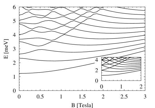
Figure 8: Main plot: Single-particle spectrum as a function of magnetic field for a non-parabolically confined dot with $\omega_{0}=1$ meV, $\gamma=1$, and $D=10a_{0}$. Remnants of shell-structure at zero field can be discerned. Inset: The same spectrum, but with $\gamma=0$, i.e., the Fock-Darwin spectrum.

The most dramatic effect of non-parabolicity is at low magnetic fields, where the shell structure is heavily renormalized, although its remnants are still observable. The plot was computed using the 1891 lowest-energy Fock-Darwin levels—corresponding, at zero field, to the first 61 shells in the parabolic case—and with $\omega_{0}=1$ meV, $\gamma=1$, and $D=10a_{0}$. At much larger $\gamma$, the shell-splitting becomes so large that different shells overlap, and a Fock-Darwin description at low fields becomes dubious. Apparent anti-crossings are also seen in Fig. 8, whereas the Fock-Darwin spectrum contains only crossings. Another important feature is that the $\nu=2$ line at moderate fields is still clearly visible, even for larger $\gamma$; beyond this point, field effects begin to play a more prominent role than non-parabolicity effects, whose presence in the spectra becomes concealed. Thus, we do not expect non-parabolicity effects to play an appreciable role beyond $\nu=2$.Ciorga et al. (2002a)

III.2.2 Interacting electrons

In section III.1, we treated the parabolically-confined interacting case by first solving for the non-interacting (Fock-Darwin) case; these states were then used as the basis states in which the interacting problem was solved. Continuing the progression, we now use the exact interacting many-body states computed in Sec. III.1 as the basis states in which we treat the non-parabolic piece of the confinement potential.

The method of truncating the Hilbert-space must again be chosen. As an example, Fig. 5—for all angular momenta since they are no longer conserved—may be considered the Hilbert-space for the particular case of $\omega_{0}=1$ meV, $B=0$ T, and $S_{z}=0$. Two methods of truncating this Hilbert-space can be considered. First, the $k$ lowest-energy states within each angular momentum channel may be chosen as the reduced Hilbert-space, with all higher-energy states discarded. For example, if $k=10$ and there are 21 angular momentum channels (as in Fig. 5), then the Hilbert space has $10\times 21=210$ dimensions. In this scheme, the cutoff energy is variable, but the number of states within each angular momentum channel is fixed. The second method is to employ a fixed energy cutoff $E_{\text{cutoff}}$ and to allow a variable number of states within each angular momentum channel; all states above $E_{\text{cutoff}}$, regardless of angular momentum, are discarded and all states below $E_{\text{cutoff}}$, regardless of angular momentum, are retained. In principle, it matters little which truncation scheme is used so long as each method, of course, converges to the same values. In practice, the second method, with a fixed cutoff energy, achieves convergence faster.

Figure 9 shows results analogous to Fig. 6, but for the non-parabolic confinement discussed above.

Figure 9: Main Plot: Singlet-triplet gap $J$ as a function of magnetic field for $\omega_{0}=1$ meV (lower curve) and $\omega_{0}=1.5$ meV (upper curve) for non-parabolically confined interacting electrons. Upper Inset: Lowest-energy singlet $|S,S_{z}\rangle=|0,0\rangle$ (lower curve) and triplet $|1,-1\rangle$ (upper curve) as a function of magnetic field for $\omega_{0}=1$ meV. Lower Inset: Shape of total confinement potential in real space. All curves in the main plot and in the insets are for $\alpha=1$, $\gamma=3$, and $D=5a_{0}$. This figure is the analog to Fig. 6 for non-parabolic confinement.

All curves shown in Fig. 9 have $(\alpha,\gamma,D)=(1,3,5a_{0})$. In the main plot, the gap $J$ is plotted for $\omega_{0}=1$ meV (lower curve) and $\omega_{0}=1.5$ meV (upper curve). The upper inset shows the singlet-triplet transition for $\omega_{0}=1$ meV, and the lower inset shows a sketch of the shape of the confinement potential for these parameter values. All these parameters, except for $\gamma$, are as in Fig. 6. The non-parabolic spectrum differs significantly from the parabolic spectrum, particularly at small field, where the triplet has a much weaker field dependence in the present case relative to the parabolic-confinement case. This is the behavior also seen in experiment. (See Fig. 2.)

In general, the non-parabolic model yields results much closer to experiment than parabolic confinement, and it is clear that the confinement potential in experiment is not parabolic. The available phase space—with variation in $\omega_{0}$, $\alpha$, $\gamma$, and $D$—is rather large and so an optimal fit has not been performed. Nevertheless, the theoretical curves in Fig. 9 are in qualitative agreement with the experimental curves in Fig. 3. Future analyses of high source-drain spectroscopy with higher electron numbers will produce additional constraints which will more meaningfully reduce the range of these parameters.

The central point is that the particular critical field $B_{c}$ obtained is itself a function of the confining-potential parameters, $\omega_{0}$, $\gamma$, and $D$. Since each of these parameters is controlled by the voltage on the gates shown in Fig. 1, it follows that the gates themselves can be used to tune through the singlet-triplet transition and hence tune the ground-state entanglement of the system. This is shown explicitly in Fig. 10 where we plot the spin phase diagram in the $\omega_{0}$-$B_{c}$ plane.

Figure 10: Spin phase diagram for the two-electron system in the $\omega_{0}$-$B_{c}$ plane. This plot has $\alpha=1$, $\gamma=3$, and $D=5a_{0}$, and $\omega_{0}$ is controlled by the gate voltages. The usual field-induced singlet-triplet transition and the voltage-induced transitions are indicated.

In this figure, the singlet-triplet gap $J$ is computed for various values of $\omega_{0}$ (tunable by the gate voltage); the critical field $B_{c}$ is then extracted from the solution to $J(\omega_{0},B_{c})\equiv 0$. In practice, the range of $\omega_{0}$ which is experimentally accessible is delimited by the $N=3$ and $N=1$ subspaces as the gate voltage is swept. However, if the accessible range is sufficient to be seen by experiment, a voltage-tuned singlet-triplet transition at fixed $B$ is achievable. As shown in Sec. II, this is indeed the case for the present experiment.

IV Discussion

The fact that the gate voltage (or set of gate voltages in the present case) controls not only the chemical potential of the dot but also the shape of the dot has been exploited in the present work to tune the ground-state entanglement of an electron pair in a lateral quantum dot. The experimental evidence clearly shows that the two-electron singlet-triplet transition occurs at a critical field which depends on the gate voltage. The confinement potential is not parabolic (nor elliptical) and this allows great flexibility in changing the shape of the dot while simultaneously keeping the number of confined electrons fixed. However, the experimental demonstration of voltage-tuned entanglement is not dependent upon the precise shape of the potential, and should be achievable in a wide range of potential shapes. The main requirement is that the gate voltages appreciably change the shape of the potential while the particle number remains constant. The present is a modest step towards the construction of a quantum gate in a solid-state environment; it does not, for example, demonstrate the unitary evolution of the system between singlet and triplet states.

Because the tunneling barriers into and out of the dot are large, only the leading order contribution to the tunneling current can be seen in our experiment. In principle, however, the tunnel barriers can be reduced while still remaining in the Coulomb blockade regime in order to measure an appreciable cotunneling current.Franceschi et al. (2001) In this way, the singlet-triplet transition may be experimentally probed throughout the $N=2$ subspace, and thus give a more stringent test of theory.

In a double-dot system with one trapped electron apiece, essentially the same spin physics occurs, and thus a voltage-tuned ground-state transition should also occur along with the consequent implications for quantum computing. Alternatively, the current work may be speculatively viewed as a possible gate-controlled single-qubit operation, where the single coded qubit exists in a single quantum dot containing two (or more) electrons. This conjecture will be more fully developed in a future publication.