Network patterns and strength of orbital currents in layered cuprates

Abstract

In a frame of the $t-J-G$ model we derive the microscopical expression for the circulating orbital currents in layered cuprates using the anomalous correlation functions. In agreement with $\mu$-on spin relaxation ($\mu$SR), nuclear quadrupolar resonance (NQR) and inelastic neutron scattering(INS) experiments in YBa₂Cu₃O_6+x we successfully explain the order of magnitude and the monotonous increase of the internal magnetic fields resulting from these currents upon cooling. However, the jump in the intensity of the magnetic fields at T_c reported recently seems to indicate a non-mean-field feature in the coexistence of current and superconducting states and the deviation of the extended charge density wave vector instability from its commensurate value Q$\approx$($\pi,\pi$) in accordance with the reported topology of the Fermi surface.

A possibility for a staggered orbital current phase formation in layered cuprates has attracted much interest recently [1, 2, 3, 4, 5, 6, 7, 8, 9, 10, 11]. Most importantly, it was shown that most of the observed properties referred to a pseudogap phenomenon can be naturally explained in an extended charge density wave (CDW) scenario with a complex order parameter phase formation (shortly $s+id$-CDW) in underdoped cuprates. The real $s-$wave symmetry component corresponds to a conventional charge (or spin) density waves whereas the imaginary part of the order parameter has a $d-$ wave symmetry and corresponds to the staggered current phase. Different kind of experiments can be interpreted in favor of the staggered orbital current phase such as an observation of the orbital antiferromagnetism in YBa₂Cu₃O_6+y by means of inelastic neutron scattering(INS) experiments reported in Refs. [5, 6] and zero-field muon spin relaxation ($\mu$sR) experiments[8]. Moreover, recent investigations using nuclear magnetic resonance (NMR) technique indicate the presence of the internal fluctuating magnetic fields in the superconducting state of layered cuprates [9, 10, 11]. Most importantly, the observed enhancement of the magnetic moment’s intensity at $T_{c}$[5, 6] seems to indicate an intrinsic and a non-trivial relation between the superconducting and the pseudogap phases. In this connection a microscopical analysis of the network patterns and the strength of orbital currents becomes very actual.

In general, the possibility of the $s+id$-CDW phase formation is related to a divergence of the dynamical charge susceptibility at wave vector ${\bf Q}_{i}\approx(\pi,\pi)$ in the first Brillouin zone and was demonstrated recently for cuprates[12]. Here we derive the analytical expression for the current flow and show how its orbital contour can be reconstructed for any arbitrary chosen instability wave vector ${\bf Q}_{i}$. Most importantly, we calculate the intensity of the resulting internal magnetic fields and the corresponding orbital magnetic moments. We find that its enhancement at $T_{c}$ may result from the presence of a relatively small $s-$component of the extended CDW. The latter agrees well with an observation of the increase of the NQR linewidth at Cu(2) site (see Ref. [11]). In addition, the non-mean-field character of the coexistence of superconductivity and $s+id$-CDW phases has to be taken into account.

Hamiltonian and general expression for the current flow. In our analysis we start from the following $t-J-G$ model Hamiltonian:

$$H=\sum_{ij}t_{ij}\Psi_{i}^{pd,\sigma}\Psi_{j}^{\sigma,pd}+\sum_{i>j}J_{ij}\left[({\bf S}_{i}{\bf S}_{j})-\frac{n_{i}n_{j}}{4}\right]+\sum_{i>j}G_{ij}\delta_{i}\delta_{j\text{ }}\quad,$$ (1)

where $\Psi_{i}^{\alpha,\beta}=\mid i,\alpha><i,\beta\mid$ are projecting Hubbard-like operators. Symbol $pd$ corresponds to a Zhang-Rice singlet formation with one hole placed on the copper site whereas the second hole is distributed on the neighboring oxygen sites [13]. Here $t_{ij}$ is a hopping integral, J_ij is a superexchange coupling parameter of copper spins, and $\sigma=\pm 1/2$. $\delta_{i}=$ $\Psi_{i}^{pd,dp}$ is a hole doping operator. As in Ref. [14] we also use the parameters of a screened Coulomb repulsion of the doped holes at different sites, $G_{ij}$. The quasiparticle energy dispersion and the correlation functions were calculated in a Roth-type of a decoupling scheme for the Green’s functions[14, 15].

The network patterns and the strength of the orbital currents can be obtained using the charge conservation low

$$\frac{\partial}{\partial t}\int\rho dV=\int\mathbf{j}d\mathbf{S}\quad.$$ (2)

The operator of the fluctuating charge per unit cell with number $i$ is given by

$$e\Psi_{i}^{pd,pd}=e\delta_{i}=\widetilde{\delta_{i}}\quad,$$ (3)

that obeys the equation of motion

$$i\hbar\frac{\partial}{\partial t}\widetilde{\delta_{i}}=\left[\widetilde{\delta_{i}}H\right]\quad.$$ (4)

Calculating the commutator with Hamiltonian (1) we arrive to the following expression

$$i\hbar\frac{\partial}{\partial t}\widetilde{\delta_{i}}=e\sum t_{ij}\Psi_{i}^{pd,\sigma}\Psi_{j}^{\sigma,pd}-e\sum t_{ji}\Psi_{j}^{pd,\sigma}\Psi_{i}^{\sigma,pd}\quad,$$ (5)

where the right-hand side of this equation is a current operator. In order to calculate its thermodynamic value along the link $<ij>$ we make the Fourier transform of Eq. (5). Then the probability of the hopping from $i$ to $j$ site can be written as:

$$<\Psi_{i}^{pd,\sigma}\Psi_{j}^{\sigma,pd}>=\frac{1}{N}\sum_{\bf k,k^{\prime}}<\Psi_{\bf k}^{pd,\sigma}\Psi_{{\bf k}^{\prime}}^{\sigma,pd}>\exp(-i{\bf kR}_{i}+i{\bf k}^{\prime}{\bf R}_{j})\quad,$$ (6)

whereas of the reverse process is given by

$$<\Psi_{j}^{pd,\sigma}\Psi_{i}^{\sigma,pd}>=\frac{1}{N}\sum_{\bf k,k^{\prime}}<\Psi_{\bf k}^{pd,\sigma}\Psi_{{\bf k}^{\prime}}^{\sigma,pd}>\exp(-i{\bf kR}_{j}+i{\bf k}^{\prime}{\bf R}_{i})\quad.$$ (7)

Since the hopping integral is a real quantity the current flow will be proportional to the difference of Eqs. (6) and (7):

$$<\Psi_{i}^{pd,\sigma}\Psi_{j}^{\sigma,pd}-\Psi_{j}^{pd,\sigma}\Psi_{i}^{\sigma,pd}>=$$ (9)

$$\frac{1}{N}\sum_{\bf k,k^{\prime}}<\Psi_{\bf k}^{pd,\sigma}\Psi_{{\bf k}^{\prime}}^{\sigma,pd}>\{\exp(-i{\bf kR}_{i}+i{\bf k}^{\prime}{\bf R}_{j})-\exp(-i{\bf kR}_{j}+i{\bf k}^{\prime}{\bf R}_{i})\}.\quad.$$

At $T<T^{*}$ one have the following non-zero expectation values: $<\Psi_{\bf k}^{pd,\sigma}\Psi_{\bf k}^{\sigma,pd}>$, $<\Psi_{\bf k+Q}^{pd,\sigma}\Psi_{\bf k}^{\sigma,pd}>$ and $<\Psi_{\bf k}^{pd,\sigma}\Psi_{\bf k+Q}^{\sigma,pd}>$. Since the first one does not contribute, we have

$$<\Psi_{i}^{pd,\sigma}\Psi_{j}^{\sigma,pd}-\Psi_{j}^{pd,\sigma}\Psi_{i}^{\sigma,pd}>=$$ (12)

$$\frac{1}{N}\sum_{\bf k,k^{\prime}}<\Psi_{\bf k+Q}^{pd,\sigma}\Psi_{\bf k}^{\sigma,pd}>\{\exp[-i({\bf k+Q}){\bf R}_{i}+i{\bf kR}_{j}]-\exp[-i({\bf k+Q}){\bf R}_{j}+i{\bf kR}_{i}]\}+$$

$$+\frac{1}{N}\sum_{\bf k}<\Psi_{\bf k}^{pd,\sigma}\Psi_{\bf k+Q}^{\sigma,pd}>\{\exp[-i{\bf kR}_{i}+i({\bf k+Q}){\bf R}_{j}]-\exp[-i{\bf kR}_{j}+i({\bf k+Q}){\bf R}_{i}\}.$$

In our case the pseudogap order parameter is expected to be the complex $(s+id)$-CDW. Therefore, it is useful to separate the correlation functions into two parts: $Re<\Psi_{\bf k+Q}^{pd,\sigma}\Psi_{\bf k}^{\sigma,pd}>$ and $Im<\Psi_{\bf k+Q}^{pd,\sigma}\Psi_{\bf k}^{\sigma,pd}>$. It is straightforward to right further as

$$<\Psi_{i}^{pd,\sigma}\Psi_{j}^{\sigma,pd}-\Psi_{j}^{pd,\sigma}\Psi_{i}^{\sigma,pd}>=$$ (15)

$$\frac{2i}{N}\sum_{\bf k}Im<\Psi_{\bf k+Q}^{pd,\sigma}\Psi_{\bf k}^{\sigma,pd}>\{\cos[{\bf kR}_{j}-({\bf k+Q}){\bf R}_{i}]-\cos[{\bf kR}_{i}-({\bf k+Q}){\bf R}_{j}]\}+$$

$$+\frac{2i}{N}\sum_{\bf k}Re<\Psi_{\bf k+Q}^{pd,\sigma}\Psi_{\bf k}^{\sigma,pd}>\{\sin[{\bf kR}_{j}-({\bf k+Q}){\bf R}_{i}]-\sin[{\bf kR}_{i}-({\bf k+Q}){\bf R}_{j}]\}.$$

For the lattice with a mirror plane symmetry perpendicular to the $x$ and $y$ axis the integrals over the first Brillouin zone containing $\sin{\bf kR}_{ji}$ vanish. Thus, in the functions $\cos[{\bf kR}_{j}-({\bf k+Q}){\bf R}_{i}]-\cos[-{\bf kR}_{i}+({\bf k+Q}){\bf R}_{j}],$ and $\sin[{\bf kR}_{j}-({\bf k+Q}){\bf R}_{i}]-\sin[-{\bf kR}_{i}+({\bf k+Q}){\bf R}_{j}]$ one can leave only their parts $\left[\cos{\bf QR}_{i}-\cos{\bf QR}_{j}\right]\cos{\bf kR}_{ji}$ and $\left[\sin{\bf QR}_{j}-\sin{\bf QR}_{i}\right]\cos{\bf kR}_{ji}$, respectively. Then, the contribution to the current flow along the $x$- axis due to the nearest hopping can be calculated:

$$J^{(1)}=\frac{e}{\hbar}t_{1}\frac{2}{N}\left[\cos{\bf QR}_{i}-\cos{\bf QR}_{j}\right]\sum_{\bf k}Im<\Psi_{\bf k+Q}^{pd,\sigma}\Psi_{\bf k}^{\sigma,pd}>\cos{\bf kR}_{ij}+$$ (17)

$$+\frac{e}{\hbar}t_{1}\frac{2}{N}\left[\sin{\bf QR}_{j}-\sin{\bf QR}_{i}\right]\sum_{\bf k}Re<\Psi_{\bf k+Q}^{pd,\sigma}\Psi_{\bf k}^{\sigma,pd}>\cos{\bf kR}_{ij}.$$

Let us discuss at the beginning the simplest case of ${\bf Q}=(\pi,\pi)$. One can immediately see that the second term of Eq. (17) vanishes. Eq. (17) allows easy to display the network patterns for the different symmetries of the order parameter ($s$-, $d$- and so on). Most importantly, for the pure d-wave symmetry order parameter $Im<\Psi_{\bf k+Q}^{pd,\sigma}\Psi_{\bf k}^{\sigma,pd}>\sim\cos k_{x}-\cos k_{y}$ (see also Ref. [16]) and hence the current network pattern is directly mapped on the well-known flux-phase state[17].

In general case the period of the current pattern is given by $a_{x}=2\pi/Q_{x}$ , $a_{y}=2\pi/Q_{y}$. Note, there are also other contributions to the network patterns due to the next-nearest- ($t_{2}$) and next-next-nearest- ($t_{3}$) neighbors hopping. These parameters are needed for the describing the real Fermi surface (see for example Ref. [18]). The contribution due to $t_{2}$ is given by

$$J^{(2)}=\frac{e}{\hbar}t_{2}\sqrt{2}\frac{2}{N}\left[\cos{\bf QR}_{i}-\cos{\bf QR}_{j}\right]\sum_{\bf k}Im<\Psi_{\bf k+Q}^{pd,\sigma}\Psi_{\bf k}^{\sigma,pd}>\cos{\bf kR}_{ij}+$$ (19)

$$+\frac{e}{\hbar}t_{2}\sqrt{2}\frac{2}{N}\left[\sin{\bf QR}_{j}-\sin{\bf QR}_{i}\right]\sum_{\bf k}Re<\Psi_{\bf k+Q}^{pd,\sigma}\Psi_{\bf k}^{\sigma,pd}>\cos{\bf kR}_{ij}\quad,$$

and due to $t_{3}$ as

$$J^{(3)}=\frac{e}{\hbar}t_{3}\frac{2}{N}\left[\cos{\bf QR}_{i}-\cos{\bf QR}_{j}\right]\sum_{\bf k}Im<\Psi_{\bf k+Q}^{pd,\sigma}\Psi_{\bf k}^{\sigma,pd}>\cos{\bf kR}_{ij}+$$ (21)

$$+\frac{e}{\hbar}t_{3}\frac{2}{N}\left[\sin{\bf QR}_{j}-\sin{\bf QR}_{i}\right]\sum_{\bf k}Re<\Psi_{\bf k+Q}^{pd,\sigma}\Psi_{\bf k}^{\sigma,pd}>\cos{\bf kR}_{ij}\quad.$$

Note in Eq. (19) indexes $i$ and $j$ refer to the next-nearest neighbors whereas in Eq. (21) $i$ and $j$ refer to the next-next-nearest neighbors.

The required correlation function can be calculated straightforwardly in a mean-field-approximation and is given by [16]:

$$<\Psi_{\bf k+Q}^{pd,\sigma}\Psi_{\bf k}^{\sigma,pd}>=\frac{P_{pd}G_{k}}{4}\left[\frac{1}{E_{1k}}\tanh\left(\frac{E_{1k}}{2k_{B}T}\right)+\frac{1}{E_{2k}}\tanh\left(\frac{E_{2k}}{2k_{B}T}\right)\right]+\frac{P_{pd}}{2(E_{1k}-E_{2k})^{2}}\times$$ (23)

$$\times\left[\frac{G_{k}}{2}(\varepsilon_{k}-\varepsilon_{k+Q})^{2}+\Delta_{k}\Delta_{k}^{*}(G_{k}+G_{k}^{*})\right]\left[\frac{1}{E_{1k}}\tanh\left(\frac{E_{1k}}{2k_{B}T}\right)-\frac{1}{E_{2k}}\tanh\left(\frac{E_{2k}}{2k_{B}T}\right)\right]$$

where

$$E_{1k,2k}^{2}=\frac{(\varepsilon_{k}+\varepsilon_{k+Q})^{2}}{2}+\Delta_{k}\Delta_{k}^{\ast}+G_{k}G_{k}^{\ast}\pm$$ (25)

$$\pm\frac{1}{2}\left[(\varepsilon_{k}^{2}-\varepsilon_{k+Q}^{2})^{2}+4G_{k}G_{k}^{\ast}(\varepsilon_{k}+\varepsilon_{k+Q})^{2}+\Delta_{k}\Delta_{k}^{\ast}(G_{k}+G_{k}^{\ast})^{2}\right]^{1/2}.$$

Here $G_{k}=S(T)+iG_{0}(T)(\cos k_{x}a-\cos k_{y}a)$ is an extended CDW gap and $\Delta_{k}=\frac{\Delta_{0}(T)}{2}(\cos k_{x}a-\cos k_{y}a)$ is a superconducting $d$-wave gap. It is important to note that the real part of the correlation function (23) contains the term which is proportional to the superconducting gap $\Delta_{k}\Delta_{k}^{\ast}$. Therefore, at T=T_c the value of the correlation function should display a ’step’ which can be responsible for the corresponding ’jump’ of the current flow. Keeping in mind this qualitative idea let us now turn to the numerical calculations.

For ${\bf Q}=(\pi,\pi)$ the resulting current is manly determined by Eq.(17). Using the equation for the $id-CDW$ order parameters in a mean field approximation (see for details Ref. [19]) it is straightforward to prove that

$$\sum_{\bf k}Im<\Psi_{\bf k+Q}^{pd,\sigma}\Psi_{\bf k}^{\sigma,pd}>\cos k_{x}a\approx\frac{G_{0}(T)}{J_{1}+2G_{1}}(1+\delta).$$ (26)

Here $J_{1,}$ and $G_{1}$ are parameters of the superexchange and the screened Coulomb repulsion of the holes at the nearest copper sites taken to be 120 meV and 135 meV respectively. $\delta$ is number of holes per one unit cell. Comparing Eq. (26) and Eq. (17) one sees that the temperature dependence of the current strength $J^{(1)}$ is almost the same as for the order parameter $G_{0}(T)$. The latter was calculated self-consistently in Ref.[16] and as was shown the results are sensitive to the details of competition between superconducting state (SC) and $id$-CDW state. Below T_c the superconductivity tries to push out $id$-CDW state and as a consequence the order parameter $G_{0}(T)$ goes down at $T<T_{c}.$ We shall describe this effect approximately as

$$G_{0}(T)=4k_{B}T_{c}x\sqrt{1-(T/T^{\ast})^{2}}-y\theta(T_{c}-T)k_{B}T_{c}\sqrt{1-(T/T_{c})^{2}}$$ (27)

where $x$ and $y$ are the parameters of coexistence of the superconducting and the $s+id$-CDW states. Here $\Delta_{0}(T)=2.4k_{B}T_{c}\sqrt{1-(T/T_{c})^{2}}$, $\theta(T_{c}-T)$ is a usual theta function and $x$ is a parameter that depends on a doping level. According to the mean field calculations [16] at $T^{*}\approx 3T_{c}$ $x$ is equal one and near the optimal doping $i.e$ when $T^{*}\approx T_{c}$, $x\approx 1/4$.

In more general case one expects that Q$\neq(\pi,\pi)$. Then the total current is a sum of $J^{(1)}+J^{(2)}+J^{(3)}$ and the relation between the current flow and the gap is not as simple as in Eq.(27). The deviation of ${\bf Q}$ from $(\pi,\pi)$ is naturally expected as a consequence of the changes in the topology of Fermi surface away from half-filling. This is also can be seen from our previous analysis of the dynamical charge susceptibility which becomes divergent along the contour around $\mathbf{Q}=$ $(\pi,\pi)$ (see for details Ref.[12]). Therefore, in Fig.1 we present the results of our calculations for the orbital currents at $\tilde{\bf Q}=(\frac{11}{12}\pi,\frac{11}{12}\pi)$ for three different regimes of co-existence of superconductivity and $s+id$-CDW phase. The gap equation yields a maximum of the critical mean field temperature of $id$-component of the pseudo-gap $(T_{d}^{*})$ (or maximum of entropy) at this $\tilde{\bf Q}$ (see Ref. [19]). Our numerical calculations show that the resulting temperature behavior of the induced magnetic field which is directly proportional to the orbital current is indeed slightly differs from the temperature dependence of the $s+id$-CDW gap. One sees from Fig. 1 that the calculated curve reproduces well the observed behavior of INS intensity[5, 6] shown in the inset. The values of the hopping integrals were chosen (in meV) t${}_{1}=100$, t${}_{2}=15$ and t${}_{3}=12$. They reproduce well the topology of the Fermi surface for underdoped cuprates.

We also would like to note the following results of our calculations. At T=T_c the jump in the current strength is reproduced only for the $x$ and $y$ values representing the non-mean field character of the coexistence phase between $s+id$-CDW and superconductivity. However, such a mean-field reduction of the effective gap at $T\leq T_{c}$ was clearly demonstrated earlier by tunneling spectroscopy[20]. Therefore weather or not a ’jump’ at $T\leq T_{c}$ exist becomes an important issue. For example there is no anomalies at T_c in $\mu$SR experiments [6], but this ’jump’ is clearly visible according to the neutron scattering data [5, 6].

Let us also comment on the importance of the small $s$-component of the extended CDW. It was shown previously that relatively small $s-$component of the extended CDW is required for the explanation of monotonic increase of the nuclear quadrupolar resonance(NQR)-Cu(2) linewidth at $T\leq T_{c}$ in YBa₂Cu₃O_6+y [11]. In this connection it is also logical to switch the $s-$component on in our discussion. This component is real and as one can see from Eqs. (19)-(23) contribute to the orbital current strength if one takes into account the deviation of instability vector ${\bf Q}$ from $(\pi,\pi)$. The values of the $s-$ component was taken as in paper [11] with critical temperature $T_{s}^{*}=100K$. As one can see the deviation effect together with $s$-component of the pseudogap can reproduce well the observed a ’jump’ at $T\leq T_{c}$ in Refs. [5, 6].

There is an additional argument in favor of the relevance $s$- component pseudogap with respect to the ’jump’ of the effective magnetic moment at $T\leq T_{c}$. It is connected with the dynamical character of the charge-current state. In fact, the discussed internal fields are not static. All experiments test the mean squared field $\sqrt{<h_{eff}^{2}>}$ that results due to an averaging dependent on how fast those fluctuations are. If the $s-$component exist the energy of the sliding $(s+id)-CDW$ condensate depends on the phase of the order parameter $G_{k}$ at $T\leq T_{c}$ and hence the sliding motion becomes decelerate. Effectively it can be viewed as an increase of the measured mean square internal magnetic fields. The situation can become even more complicated because, as it was stressed recently the appearance of the $s-$component of CDW leads to a damping of the quasiparticle regime[9]. In other words one can say that the appearance of the $s-$ components of CDW stimulate the nano-scale localization phenomenon. The relation of the disorder to the problem of the local magnetic fields in YBa₂Cu₃O_6+y from experimental point of view was stressed also very recently[21].

Finally we note that the current network pattern, corresponding to the case of ${\bf Q}=0$ was discussed by Varma [22]. We do not touch this case here because according to the neutron scattering data the ${\bf Q}$ is about $(\pi,\pi)$. Therefore this case seems to be less actual. Further experimental studies are required in order to verify the orientation of the observed magnetic moments. According to Ref.[5] they are aligned along $c$-axis (this is in agreement with our discussed $(s+id)$-CDW scenario), whereas Sidis et al.,[6] reports the polarization of the magnetic moments in the copper-oxygen plane.

In summary, the observed monotonously increasing of the magnetic moment by neutron scattering[5, 6] is well reproduced our calculations if one identifies the temperature of $T^{*}$ around 300 K as a critical temperature of $(s+id)$-CDW phase formation. This value is correlated with those $T^{*}$ that were reported earlier as a pseudogap temperature in these compounds. We argue that the reported jump in the intensity at $T=T_{c}$ can be attributed to the presence of the relatively small $s-$component of the pseudogap due to deviation of the CDW instability vector Q from $(\pi,\pi)$. The latter results from the observed topology of the Fermi surface and the corresponding behavior of the dynamical charge susceptibility in underdoped cuprates[12].

We are thankful for stimulating discussions with A. Dooglav, A. Rigamonti, and D. Manske. This work was supported by the Swiss National Science Foundation (Grant No. 7SUPJ062258) and partially by the Russian Scientific Council on Superconductivity (Project No. 98014-1). I.E. was supported by the Alexander von Humboldt Foundation.

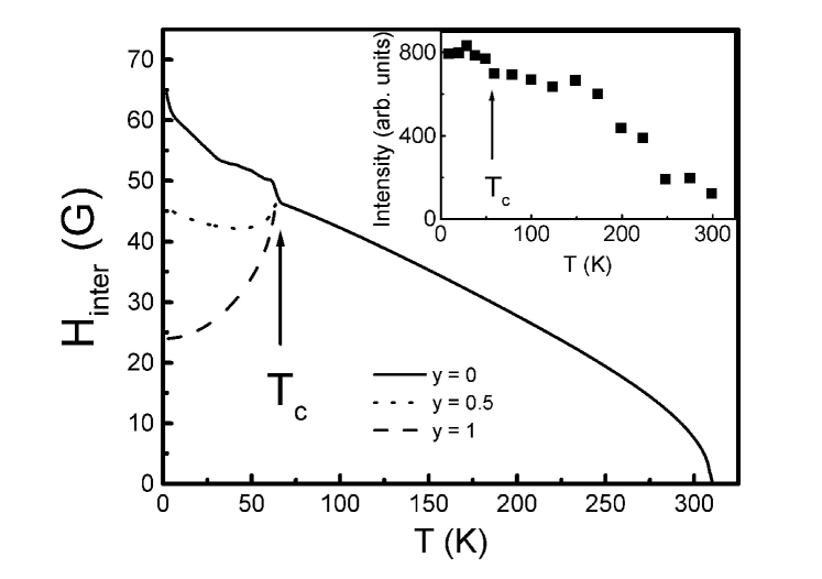
FIG. 1.: Calculated intensity of the orbital currents in units of the magnetic field[17] H${}_{int}=\frac{J^{(1)}+J^{(2)}+J^{(3)}}{\hbar cr}$ (where $r\approx 2\dot{A}$) at $\tilde{\bf Q}=(\frac{11}{12}\pi,\frac{11}{12}\pi)$ for three different regimes of the co-existence between extended CDW and superconductivity as described in the text. Inset shows the experimental data taken from Ref. [5].

REFERENCES

- [1] S. Chakravarty, R.B. Laughlin, D.K. Morr, and Ch. Nayak, Phys. Rev. B63, 094503 (2001).
- [2] S. Tewari, H.-Y. Kee, Ch. Nayak, and S. Chakravarty, Phys. Rev. B64, 224516 (2001).
- [3] S. Chakravarty, H.-Y. Kee, and Ch. Nayak, Int. J. Mod. Phys. B 15, 2901 (2001).
- [4] J.O. Fajerestad and J.B. Marston, cond-mat/0107094 (unpublished) (2001).
- [5] H.A. Mook, P. Dai, and F. Dogan, Phys Rev. B64, 012502 (2001).
- [6] Y. Sidis, C. Ulrich, Ph. Bourges, C. Bernhard, C.Niedermayer, L.P. Regnault, N.H. Andersen, and B. Keimer, Phys Rev. Lett. 86, 4100 (2001).
- [7] J.A. Hodges, Y. Sidis, Ph. Bourges, I. Mirebeau, M. Hennion, X. Chaud, cond-mat/0107218 (unpublished) (2001).
- [8] J.E. Sonier, J.H. Brewer, R.F. Kiess, R.I. Miller, G.D. Morris, C.E. Stronach, J.S. Gardner, S.R. Dunsiger, D.A. Bonn, W.N. Hardy, R. Liang, and R.H. Heffner, Science 292, 1692 (2001).
- [9] M.V. Eremin and A. Rigamonti, Phys. Rev. Lett., to be published (cond-mat/0103282).
- [10] M.V. Eremin, Yu.A. Sakhratov, A.V. Savinkov et al., Pis’ma Zh. Eksp. Teor. Fiz. 73, 609 (2001) JETP Lett. 73, 540 (2001).
- [11] A.V. Dooglav, M.V. Eremin, Yu.A. Sakhratov, and A.V. Savinkov, Pis’ma Zh. Eksp. Teor. Fiz. 74, 108 (2001) JETP Lett. 74, 103 (2001).
- [12] M. Eremin, I. Eremin, and S. Varlamov, Phys. Rev B64, 214512 (2001).
- [13] F.C. Zhang and T.M. Rice, Phys. Rev. B37, 3757 (1988).
- [14] M.V. Eremin et al., JETP Lett. 60, 125 (1994); J.Phys. Chem. Solids. 56, 1713 (1995).
- [15] N.M. Plakida, R. Hayn, and J.L. Richard, Phys. Rev. B51, 16599 (1995).
- [16] M.V. Eremin and I.A. Larionov, Pis’ma Zh. Eksp. Teor. Fiz. 68 583 (1998) [JETP Lett. 68, 611 (1998)].
- [17] T.S. Hsu, J.B. Marston, and I. Affleck, Phys. Rev. B43, 2866 (1991).
- [18] M.R. Norman, Phys. Rev. B61, 14751 (2000).
- [19] I. Eremin and M. Eremin, J. Supercond. 10, 459 (1997); S. Varlamov, M.Eremin, and I. Eremin, Pis’ma Zh. Eksp. Teor. Fiz. 66, 533 (1997) [JETP Lett. 66, 569 (1997)].
- [20] T. Ekino, Y. Sezaki, and H. Fujii, Phys. Rev. B60, 6916 (1999).
- [21] J.E. Sonier, J.H. Brewer, R.F. Kiefl, R.H. Heffner, K. Poon, S.L. Stubbs, G.D. Morris, R.I. Miller, W.N. Hardy, R. Liang, D.A. Bonn, J.S. Gardner, and N.J. Curro, cond-mat/0108479 (unpublished).
- [22] C. Varma, Phys. Rev. Lett. 83, 3538 (1999).