Quantum corrections to conductivity: from weak to strong localization

Abstract

Results of detailed investigations of the conductivity and Hall effect in gated single quantum well GaAs/InGaAs/GaAs heterostructures with two-dimensional electron gas are presented. A successive analysis of the data has shown that the conductivity is diffusive for $k_{F}l=25-2$. The absolute value of the quantum corrections for $k_{F}l=2$ at low temperature is not small, e.g., it is about $70$ % of the Drude conductivity at $T=0.46$ K. For $k_{F}l=2-0.5$ the conductivity looks like diffusive one. The temperature and magnetic field dependences are qualitatively described within the framework of the self-consistent theory by Vollhardt and Wölfle. The interference correction is therewith close in magnitude to the Drude conductivity so that the conductivity $\sigma$ becomes significantly less than $e^{2}/h$. We conclude that the temperature and magnetic field dependences of conductivity in the whole $k_{F}l$ range are due to changes of quantum corrections.

I Introduction

The weak localization regime in two-dimensional (2D) systems at $k_{F}l\gg 1$ ($k_{F}$ and $l$ are the Fermi quasimomentum and mean free path, respectively), when the electron motion is diffusive, is well understood from theoretical point of view.Altshuler In this case the quantum corrections to conductivity, which are caused by electron-electron interaction and interference, are small compared with the Drude conductivity $\sigma_{0}=\pi G_{0}k_{F}l$, where $G_{0}=e^{2}/(2\pi^{2}\hbar)$. Experimentally, this regime was studied in different types of 2D systems. Qualitative and in some cases quantitative agreement with the theoretical predictions was found. However, important questions remain to be answered: (i) what does happen with these corrections at decrease of $k_{F}l$ down to $k_{F}l\simeq 1$ and (ii) at decrease of temperature $T$ when the quantum corrections become comparable in magnitude with the Drude conductivity?

It is clear that the increase of disorder sooner or later leads to the change of the conductivity mechanism from diffusive one to hopping and another question is: when does it happen? To answer this question the temperature dependence of the conductivity is analyzed usually. It is supposed that the transition to the hopping conductivity occurs when the conductivity becomes lower than $e^{2}/h$ and the strong temperature dependence arises.h1 ; h2 ; h3 ; h4 ; h5 From our point of view, it is not enough to analyze only the $\sigma(T)$ dependence. The low conductivity and its strong temperature dependence can result from large value of the quantum corrections as well.

The aim of this paper is to study the role of quantum corrections over wide range of $k_{F}l$ and to understand what happens when the quantum corrections become comparable with the Drude conductivity. We try to answer these questions studying the quantum corrections in the 2D systems with the simplest and well-known electron energy spectrum, starting from the well understandable case $k_{F}l\gg 1$.

We report experimental results obtained for gated single quantum well GaAs/InGaAs/GaAs structures with one 2D subband occupied. An analysis of the experimental data shows that the conductivity is diffusive when $k_{F}l$ varies from $25$ to approximately $2$ and looks like diffusive one at $k_{F}l=2-0.5$. At low temperature and $k_{F}l\simeq 1$ the total quantum correction is not small. It is close in magnitude to the Drude conductivity so that the conductivity is significantly less than $e^{2}/h\simeq 3.86\times 10^{-5}$ $\Omega^{-1}$ at low temperature: for instance, for $k_{F}l\simeq 0.5$ it is about $3\times 10^{-8}$ $\Omega^{-1}$ at $T=0.46$ K, that is six hundred odd times less than $\sigma_{0}$. Thus, in this range the strong temperature and magnetic field dependences are caused by the change of quantum corrections.

II samples

The heterostructures investigated were grown by metal-organic vapor-phase epitaxy on a semiinsulator GaAs substrate. They consist of $0.5$-mkm-thick undoped GaAs epilayer, a Sn $\delta$ layer, a 60-Å spacer of undoped GaAs, a 80-Å In_0.2Ga_0.8As well, a 60-Å spacer of undoped GaAs, a Sn $\delta$ layer, and a 3000-Å cap layer of undoped GaAs. The samples were mesa etched into standard Hall bars with the dimensions $1.2\times 0.2$ mm² and then the gate electrode was deposited onto the cap layer by thermal evaporation. The measurements were performed in the temperature range $0.4-12$ K at magnetic field $B$ up to 6 T. The electron density was found from the Hall effect and from the Shubnikov-de Haas oscillations where it was possible. These values coincide with an accuracy of 5%.

The gate voltage dependences of the electron density and conductivity are presented in Fig. 1(a), (b). Varying the gate voltage $V_{g}$ from $0.0$ to $-3.3$ V we changed the electron density in the quantum well from $7.5\times 10^{11}$ to $1.2\times 10^{11}$ cm^-2 and the conductivity $\sigma$ at $T=4.2$ K from $2.1\times 10^{-3}$ to $6\times 10^{-7}$ $\Omega^{-1}$. The straight line in Fig. 1(a) shows the $V_{g}$-dependence of the total electron density in the quantum well and $\delta$ layers, calculated from the simple electrostatic consideration: $n_{t}(V_{g})=n(0)+V_{g}\,C/|e|$ with $n(0)$ as fitting parameter. Here, $C$ is the gate-2D channel capacity per centimeter squared $C=\varepsilon/(4\pi d)$, where $d=3000$Å is the cap-layer thickness and $\varepsilon=12.5$. The deviation of the experimental data from the line, which is evident at $V_{g}>-1$ V is a result of that the fraction of electrons occupies the states in $\delta$ layers. Arising of the electrons and, hence, empty states at the Fermi energy in $\delta$ layers leads to specific features in transport, Tau-phi that need an additional detailed investigation and will be discussed elsewhere.

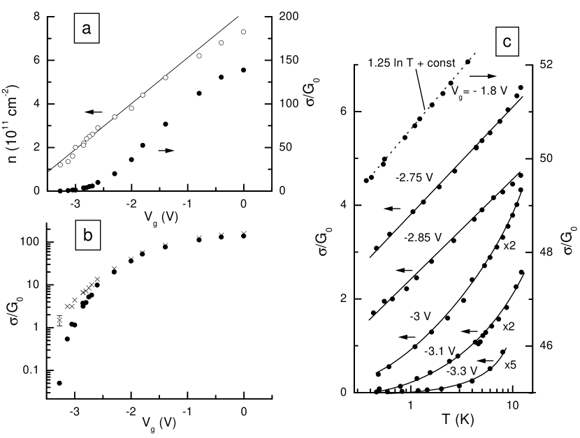
Figure 1: (a) The gate voltage dependence of the conductivity at $T=4.2$ K (solid circles) and electron density in quantum well (open circles). The line is the dependence $n_{t}(V_{g})$ calculated from the electrostatic consideration (see text). (b) The gate voltage dependences of conductivity at $T=4.2$ K (circles) and the Drude conductivity (crosses). (c) Temperature dependences of the conductivity for different gate voltages. The solid lines are the guide for an eye, dotted line is Eq. (8) with $(1+3/4\lambda)=0.35$ and $p=0.9$ (see text).

III Results and discussion

The temperature dependences of the conductivity for some gate voltages are presented in Fig. 1(c). It is clearly seen that for $V_{g}\geq-2.85$ V the temperature dependences of $\sigma$ are close to the logarithmic ones. For lower $V_{g}$, when the conductivity is less than $e^{2}/h$, the significant deviation from logarithm is evident. The conductivity in this range is usually interpreted as the hopping conductivity. h1 ; h2 ; h3 ; h4 ; h5 Below we will show that the quantum corrections can lead to such a behavior if they become close in magnitude to the Drude conductivity.

To clarify the role of quantum corrections at low conductivity when $k_{F}l\simeq 1$ let us analyze the experimental data starting from $k_{F}l\gg 1$ when the conventional theories of the quantum corrections are applicable. Following the sequence of data treatment described in Ref. e-e, we will assure at first that the quantum correction theories describe temperature, low and high magnetic field behavior of the conductivity. After that we will find the contributions of the electron-electron interaction and quantum interference to the conductivity and then trace their changes with lowering of $k_{F}l$.

III.1 The case $k_{F}l\gg 1$

In Fig. 2 the magnetic field dependences of $\rho_{xx}$ and $\rho_{xy}$ taken at different temperatures for gate voltage $V_{g}=-1.8$ V are presented. The two different magnetic field ranges are evident in Fig. 2(a): the range of sharp decrease of $\rho_{xx}$ at low field $B\leq 0.1-0.2$ T, and the range of moderate dependence at higher field. All the $\rho_{xx}$-versus-$B$ curves cross each other at fixed magnetic field $B_{cr}$.

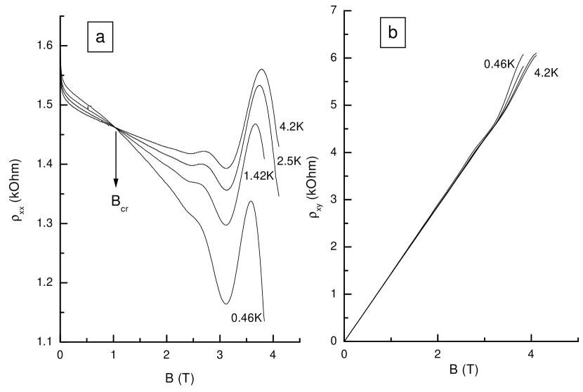
Figure 2: The magnetic field dependences of $\rho_{xx}$ (a) and $\rho_{xy}$ (b) for different temperatures at $V_{g}=-1.8$ V ($k_{F}l=17.9$).

The high-magnetic field behavior of $\rho_{xx}$ fully corresponds to the theory for electron-electron interactionAltshuler which predicts that

$$\delta\sigma_{xx}^{ee}(T) = G_{0}\left(1+\frac{3}{4}\lambda\right)\ln\left(\frac{kT\tau}{\hbar}\right)$$ (1)

$$\delta\sigma_{xy}^{ee} = 0$$ (2)

and hence

$$\rho_{xx}(B,T)\simeq\frac{1}{\sigma_{0}}-\frac{1}{\sigma_{0}^{2}}\left(1-\mu^{2}B^{2}\right)\delta\sigma_{xx}^{ee}(T),$$ (3)

when $\delta\sigma_{xx}^{ee}\ll\sigma_{0}$. Here, $\tau$ is the quasimomentum relaxation time, and $\lambda$ is the parameter of electron-electron interaction. The value of $\lambda$ has been calculated in Ref. Fin, and found being independent of the magnetic field when $g\mu_{B}B\leq kT$. It is clearly seen from Eq. (3) that $\rho_{xx}$-versus-$B$ plots measured for different temperatures have to cross each other at magnetic field $B=\mu^{-1}$. Experimentally, the value of $B_{cr}=1$ T is really close to $1/\mu$ with $\mu=0.99$ m${}^{2}/(\text{V}\times\text{sec})$.

The temperature dependences of $\sigma_{xx}$ and $\sigma_{xy}$ for high magnetic field are presented in Fig. 3. As seen $\sigma_{xy}$ is temperature independent within an experimental error. The temperature dependence of $\sigma_{xx}$ is close to the logarithmic one. The slope of the $\sigma_{xx}$-versus-$\ln\,T$ plot does not depend on the magnetic field. Thus, the high magnetic field behavior of conductivity tensor components agrees completely with the theoretical predictions for the correction due to electron-electron interaction. It allows us to determine the value of $(1+3/4\lambda)$ [see Eq. (1)]. So, for $V_{g}=-1.8$ V we obtain $(1+3/4\lambda)=0.35\pm 0.05$.

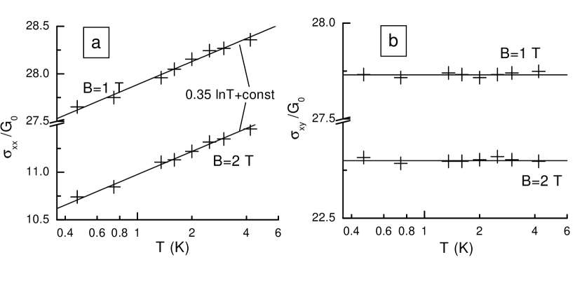
Figure 3: Temperature dependence of $\sigma_{xx}$ (a) and $\sigma_{xy}$ (b) for two magnetic fields, $V_{g}=-1.8$ V

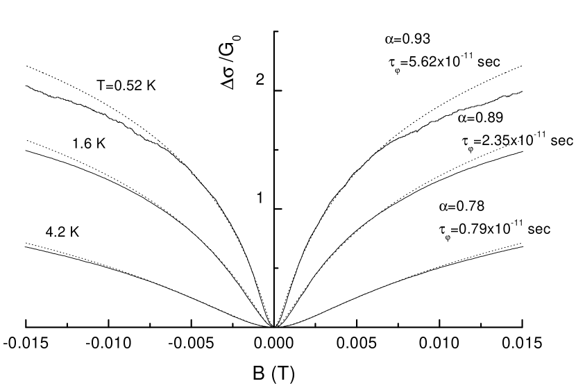
Figure 4: The magnetic field dependence of $\Delta\sigma(B)=1/\rho_{xx}(B)-1/\rho_{xx}(0)$ for different temperatures, $V_{g}=-1.8$ V. Solid curves are the experimental data. Dashed lines are the best fit to Eq. (4) made over the magnetic field range from 0 to $0.25\,B_{tr}$, $B_{tr}=0.03$ T. The parameters of the best fit are given near the corresponding curves.

We turn now to the low-magnetic-field behavior of $\rho_{xx}$, which is a consequence of suppression of the interference correction by magnetic field (Fig. 4). At $B<0.5B_{tr}$, where $B_{tr}=\hbar/(2el^{2})$,ftn1 the dependences $\Delta\sigma(B)=1/\rho_{xx}(B)-1/\rho_{xx}(0)$ are described by the well-known expressionHik

$$\Delta\sigma(B) = \alpha G_{0}\biggl{\{}\psi\left(\frac{1}{2}+\frac{\tau}{\tau_{\varphi}}\frac{B_{tr}}{B}\right)$$ (4)

$$- \psi\left(\frac{1}{2}+\frac{B_{tr}}{B}\right)-\ln{\left(\frac{\tau}{\tau_{\varphi}}\right)}\biggr{\}}$$

with $\alpha$ and $\tau_{\varphi}$ given in this figure. In Eq. (4), $\psi(x)$ is a digamma function, $\tau_{\varphi}$ is the phase breaking time. A difference of the prefactor $\alpha$ from unity, which is more pronounced at higher temperature, is sequence of low ratio $\tau_{\varphi}/\tau$. For instance, $\tau_{\varphi}/\tau\simeq 20$ for $T=4.2$ K. It is apparently not enough for the diffusion approximation.our1 Nevertheless, as shown in Ref. our1, the use of Eq. (4) for the fit of experimental data in this regime gives the value of $\tau_{\varphi}$ very close to the true one.

If one plots the temperature dependence of $\tau_{\varphi}$ found from the fit, we obtain it being close to $T^{-p}$ with $p\simeq 0.9$ (Fig. 5), which is close to the theoretical value $p=1$:

$$\tau_{\varphi}^{-1}=\frac{kT}{\hbar}\frac{2\pi G_{0}}{\sigma_{0}}\ln\left(\frac{\sigma_{0}}{2\pi G_{0}}\right).$$ (5)

Notice, that not only the temperature dependence but the absolute value of $\tau_{\varphi}$ obtained experimentally is close to the theoretical one.

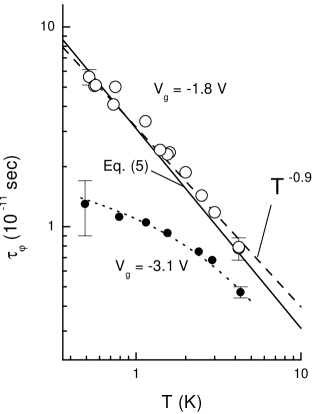
Figure 5: The temperature dependences of $\tau_{\varphi}$ at $V_{g}=-1.8$ V, $k_{F}l=17.9$ (open circles) and $V_{g}=-3.1$ V, $k_{F}l\simeq 1$ (solid circles). Solid line is the theoretical dependence given by Eq. (7), dashed line is the power law $T^{-0.9}$, dotted line is the guide for an eye.

So, we can determine the absolute value of the interference correction at $B=0$ using the well-known expression

$$\delta\sigma^{int}=-G_{0}\ln\left(\frac{\tau_{\varphi}}{\tau}+1\right).$$ (6)

Fig. 6 shows the results obtained for $T=0.46$ K. As seen $\delta\sigma^{int}$ is practically independent of $k_{F}l$ while $k_{F}l\geq 2$.

Now, when we have experimentally found the values of both electron-electron and interference contributions to the conductivity, we can determine the total value of quantum corrections $\delta\sigma(T)=\delta\sigma^{int}(T)+\delta\sigma^{ee}(T)$ and the value of the Drude conductivity:

$$\sigma_{0}=\sigma(T)-\delta\sigma(T).$$ (7)

If the experimental results are adequately described by the theory of the quantum corrections we have to obtain the same values of $\sigma_{0}$ from the data taken at different temperatures. Really, this procedure gives the close values. The scatter is about $(0.5-1)\,G_{0}$ for $T=0.46-10$ K in the whole gate voltage range. The Drude conductivity obtained by this way as a function of $V_{g}$ is presented in Fig. 1 (b).

The found value of $\sigma_{0}$ can be further compared with $\rho_{xx}^{-1}(B_{cr})$. Both quantities have to be equal each other as it follows from Eq. (3). As an example we consider the case of $V_{g}=-1.8$ V. The value of $\sigma_{0}$ obtained with the help of Eq. (7) is equal to $(56.4\pm 0.5)\,G_{0}$. Inspection of Fig. 2 gives $\rho_{xx}(B_{cr})^{-1}=55.6\,G_{0}$. It is slightly lower than $\sigma_{0}$. The reason for this difference is transparent.e-e It is due to the remainder of the interference correction which is not fully suppressed by magnetic field even at $B=B_{cr}\simeq 30\,B_{tr}$.

Finally, the temperature dependence of the conductivity at zero magnetic field is determined by the overall temperature dependences of $\delta\sigma_{xx}^{ee}$ [Eq. (1)] and $\delta\sigma^{int}$ [Eq. (6)]. Thus,

$$\sigma(T)\propto G_{0}\left(1+\frac{3}{4}\lambda+p\right)\ln\,T.$$ (8)

The dotted line in Fig. 1(c) demonstrates a good agreement of the experimental data with Eq.(8) when one uses $(1+3/4\lambda)=0.35$ and $p=0.9$ obtained above.

As is clear from above the cross of $\rho_{xx}(B)$ for different $T$ is essential for the thorough analysis. Unfortunately the cross point is observed not over the whole gate voltage range because the decreasing of $V_{g}$ leads to mobility decrease and hence to shift of $B_{cr}$ to high magnetic field. At $V_{g}<-2.9$ V the cross is out the used magnetic field range. But at $V_{g}>-2.9$ V wherever the cross is evident the good agreement with all the theoretical predictions takes place. The minimal value of $k_{F}l$ therewith is about 2.

Besides, Eq. (3) is valid when one can ignore the quantization of the energy spectrum in a magnetic field, i.e., when the cyclotron energy $\hbar\omega_{c}$ is less than the broadening of the Landau levels or the Fermi energy. In the structure investigated $\hbar\omega_{c}$ at $B=\mu^{-1}$ is less than the Fermi energy while $n>2\times 10^{11}$ $\text{cm}^{-2}$ that corresponds to $k_{F}l>2$.

Thus, we maintain that at $k_{F}l\gtrsim 2$ just the quantum corrections determine the temperature, low and high magnetic field dependences of the conductivity in two-dimensions. The total value of the corrections decreases only slightly at decreasing $k_{F}l$ (see Fig. 6), the contribution due to electron-electron interaction is 25-30 % of the interference contribution at $k_{F}l\simeq 25$ and only 10 % at $k_{F}l\simeq 2$. The significant point is that the quantum corrections at low temperature can be comparable in magnitude with the Drude conductivity, e.g., at $k_{F}l=2.3$ ($V_{g}=-2.85$ V), their value is about two-third of $\sigma_{0}$ when $T=0.46$ K. So, the strong enough temperature dependence of the conductivity at $B=0$ in this case (see Fig. 1 (c)) is caused by the decreasing of the quantum corrections with temperature.

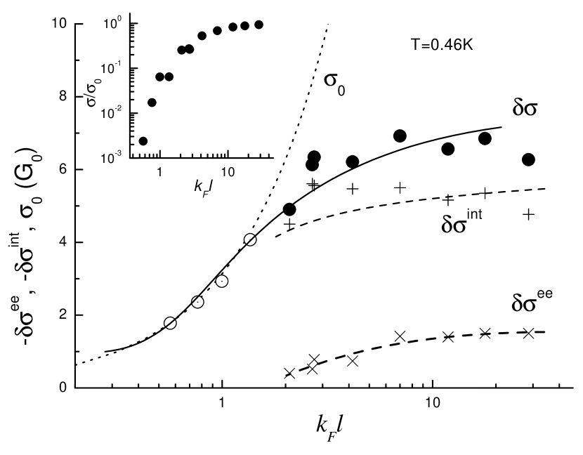
Figure 6: The contributions to the conductivity due to electron-electron interaction $\delta\sigma^{ee}$, interference $\delta\sigma^{int}$, and the total contribution $\delta\sigma$ as a function of $k_{F}l$. The dotted curve is $\sigma_{0}=\pi k_{F}l$, other curves are the guide for an eye. Solid and open circles are obtained as described in Sec. III.1 and Sec. III.2, respectively. Inset shows the ratio of the conductivity in zero magnetic field at $T=0.46$ K to the Drude conductivity plotted as a function of $k_{F}l$.

Now we consider the behavior of the electron-electron contribution with $k_{F}$ changing. In Fig. 7 the experimental $k_{F}$-dependences of $(1+3/4\lambda)$ obtained for structure investigated together with the theoretical curveFin are presented. One can see that at $2k_{F}/K>1.5$ ($K$ is the screening parameter) when $k_{F}l>5$ the experiment lies somewhat below the theoretical curve. Over this range of $2k_{F}/K$ our results are close to those from Ref. e-e, . The strong deviation of $(1+3/4\lambda)$ at $2k_{F}/K<1.5$ can be result of the low value of $k_{F}l$ whereas the theory has been developed for $k_{F}l\gg 1$.

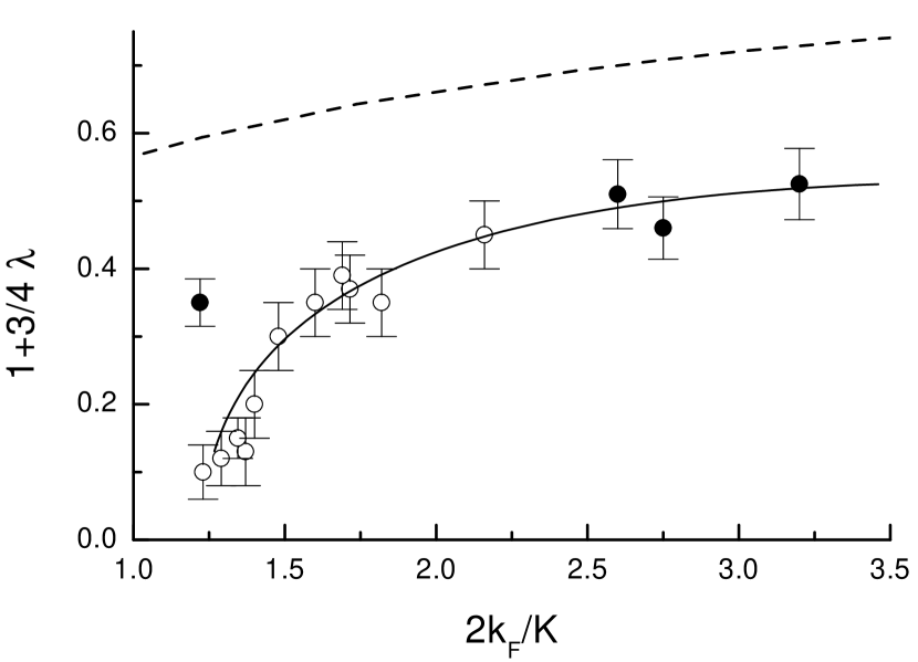
Figure 7: The value of multiplier $\left(1+3/4\lambda\right)$ in Eq. (1) as a function of $2k_{F}/K$. The open circles are the results obtained for structure investigated, the solid circles are the results from Ref. e-e, . The dashed curve represents the theoretical result from Ref. Fin, . Solid curve is the guide for an eye.

III.2 The case $k_{F}l\simeq 1$

Let us analyze the data for $V_{g}<-2.9$ V when the conductivity is low and the cross point is not observed. First of all, one can see from Fig. 1 (c) that the temperature dependence of $\sigma$ is not logarithmic in this case. It is not surprising because Eqs. (1) and (6) are valid when the corrections are small compared with the Drude conductivity. When the temperature tends to zero, Eq. (7) together with Eqs. (1) and (6) gives the negative value of the conductivity that is meaningless. It is obvious that another theoretical approach should be used in this situation. Self-consistent calculationsVoelfle ; Gogolin lead to the equation for the conductivity

$$\frac{\sigma(T)}{\sigma_{0}}=1-\frac{1}{\pi k_{F}l}\ln\left(1+\frac{\tau_{\varphi}(T)}{2\tau}\frac{\sigma(T)}{\sigma_{0}}\right).$$ (9)

When $\tau_{\varphi}\gg\tau$ it can be rewritten as

$$\frac{\sigma_{0}}{G_{0}}+\ln\left(\frac{\sigma_{0}}{G_{0}}\right)-\left[\frac{\sigma(T)}{G_{0}}+\ln\left(\frac{\sigma(T)}{G_{0}}\right)\right]=\ln\left[\frac{\tau_{\varphi}(T)}{\tau}\right].$$ (10)

This equation coincides with Eq. (6) if $\sigma_{0}-\sigma(T)\ll\sigma_{0}$, and at $\tau_{\varphi}(T)/\tau$ going to the infinite gives $\sigma(T)$ going to zero. In Fig. 8 we present our experimental results as $[\sigma(T)/G_{0}+\ln(\sigma(T)/G_{0})]$-versus-$\ln T$ plot in accordance with Eq. (10). It is evident the experimental data are well described by this theory.

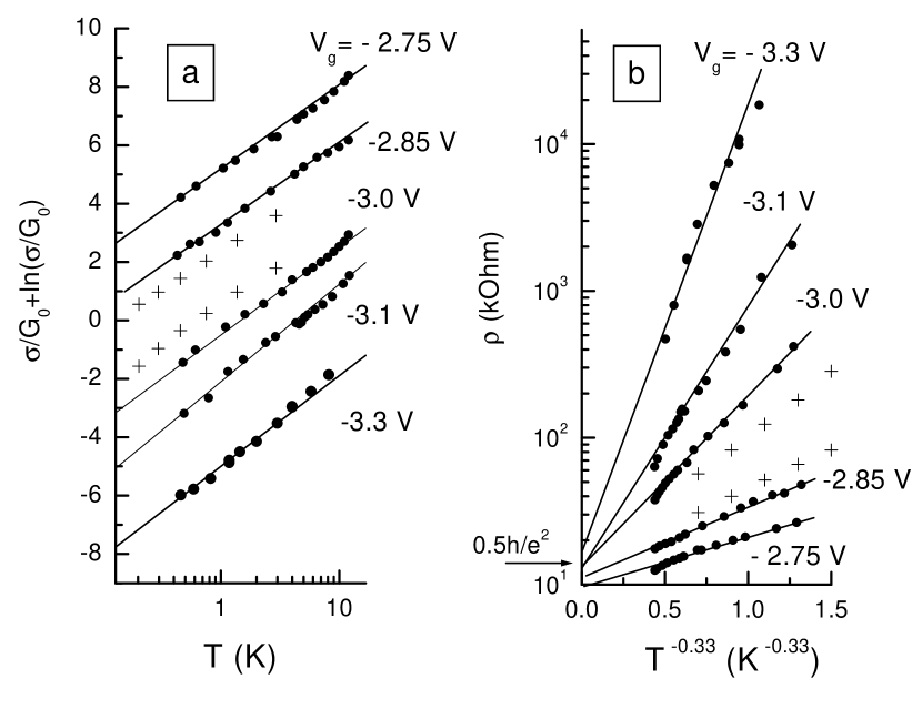
Figure 8: The temperature dependence of $\sigma$ (a) and $\rho$ (b) in the coordinates corresponding to Eqs. (10) and (11) with $m=1/3$ respectively. The circles are our data, the crosses are results from Ref. h5, . The values of $k_{F}l$ from $V_{g}=-2.75$ V to $-3.3$ V are the following: $k_{F}l\simeq 3$; $2.1$; $1.4$; $1.0$; and $0.5$.

Moreover, the negative magnetoresistance is observed in this range too. Notice, the shape of $\Delta\sigma$-versus-$B$ dependence is the same as for large $k_{F}l$. It is illustrated by Fig. 9 where $\Delta\sigma$-versus-$B$ data for $V_{g}=-1.8$ V ($k_{F}l=17.9$) and $V_{g}=-3.3$ V ($k_{F}l\simeq 0.5$, see below for details) are presented. It is evident that both data sets practically coincide. From our point of view this fact indicates that at both small and large $k_{F}l$-value the negative magnetoresistance results from the magnetic-field suppression of the interference correction to the conductivity.

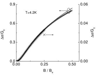
Figure 9: The negative magnetoresistance for $V_{g}=-1.8$ V ($k_{F}l=17.9$) (circles) and $V_{g}=-3.3$ V ($k_{F}l\simeq 0.5$) (crosses), $T=4.2$ K.

Let us try to determine the phase breaking time from the negative magnetoresistance. By analogy with the temperature dependence of $\sigma$ [see Eq. (10)] we have analyzed the magnetic filed dependence of $\sigma(B)/G_{0}+\ln[\sigma(B)/G_{0}]-[\sigma(0)/G_{0}+\ln[\sigma(0)/G_{0}]]$ rather than $\sigma(B)-\sigma(0)$ as was in Eq. (4). Note, that the way of finding the value of $B_{tr}$ used in the case $k_{F}l\gg 1$ (see Ref. ftn1, ) is pure now because $\sigma$ strongly differs from $\sigma_{0}$. Therefore, we used successive approximation method. For the first approximation we have used $\sigma(0)$ as $\sigma_{0}$, found $B_{tr}$ and, than, determined $\tau_{\varphi}/\tau$ from the fit of magnetoresistance. After that we have substituted this ratio into Eq. (10) and found the corrected value of $\sigma_{0}$ and so on. So, output of this procedure is the value of the Drude conductivity $\sigma_{0}$ and the ratio $\tau_{\varphi}/\tau$.

We realize that Eqs. (4) and (10) have been used beyond the framework of their workability. Nevertheless, let us consider the results. It has been found that the lowering of $V_{g}$ down to $-3.3$ V leads to the fall of the Drude conductivity down to $\simeq 1.5\,G_{0}$ [see Fig. 1 (b)], that is, $k_{F}l\simeq 0.5$. The values of fittimg parameters $\tau_{\varphi}$ and $\alpha$ therewith change slowly and monotonically over the whole $k_{F}l$-range. It is clearly seen from Fig. 10 in which the results for $k_{F}l>2$ described in Sec. III.1 are presented as well. Moreover, $\tau_{\varphi}$ behaves naturally with temperature: it increases with temperature decrease (Fig. 5).

Finally, knowing the Drude conductivity we can find the total value of quantum corrections as $\delta\sigma(T)=\sigma(T)-\sigma_{0}$. For $T=0.46$ K, the value of $\delta\sigma$ as a function of $k_{F}l$ is depicted in the Fig. 6. As the figure illustrates, these results match those obtained for $k_{F}l>2$ and discussed in previous subsection. It is seen that the total quantum correction $\delta\sigma$ is small part of the Drude conductivity $\sigma_{0}$ at large $k_{F}l$, is about 70% of $\sigma_{0}$ at $k_{F}l\simeq 2$, and very close to $\sigma_{0}$ at lower $k_{F}l$. The last leads to the fact that at low temperature the conductivity in zero magnetic field is very small fraction of the Drude conductivity (see inset in Fig. 6). For instance, $\sigma/\sigma_{0}\simeq 2\times 10^{-3}$ at $k_{F}l\simeq 0.5$ and $T=0.46$ K, the absolute value of $\sigma$ is about $3\times 10^{-8}$ $\Omega^{-1}$ that is much smaller than $e^{2}/h\simeq 3.86\times 10^{-5}\,\Omega^{-1}$.

Thus, down to $k_{F}l\simeq 0.5$ the conductivity looks like diffusive one and its temperature and magnetic field dependence is due to that of the quantum corrections which can be comparable in magnitude with the Drude conductivity at low temperature.

It is usually supposed that at $\sigma<e^{2}/h$ the conductivity mechanism is the variable range hopping.h1 ; h2 ; h3 ; h4 ; h5 It is argued by the fact that the temperature dependence of the resistivity $\rho=\sigma^{-1}$ is well described by characteristic for this mechanism dependence:

$$\rho(T)=\rho_{0}\exp{\left(\frac{T_{0}}{T}\right)^{m}}$$ (11)

with $m=1/2,1/3$ depending on the ratio of the Coulomb gap width to the temperature. Fig. 8 (b) shows our experimental results as $\ln\rho$-versus-$T^{-1/3}$ plot. As seen our data being in an excellent agreement with Eq. (10) [Fig. 8 (a)] are well described by Eq. (11) too. Surprised by this fact we have examined some data from Refs. h1, ; h2, ; h3, ; h4, ; h5, , which were interpreted from the position of the variable range hopping. We have found that while the resistivity is less than $\sim 10^{6}$ $\Omega$ those dependences are well aligned in $[\sigma(T)/G_{0}+\ln(\sigma(T)/G_{0})]$-versus-$\ln T$ coordinates also. For example, in Fig. 8 the data from Ref. h5, for carrier density $1.085\times 10^{11}$ and $0.984\times 10^{11}$ cm^-2 are presented. Thus only the temperature dependence of the conductivity does not allow to identify the conductivity mechanism reliably.

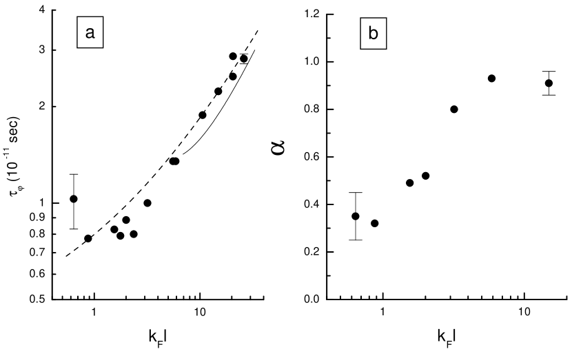
Figure 10: The conductivity dependence of $\tau_{\varphi}$ (a) and prefactor $\alpha$ (b) at $T=1.5$ K. Symbols are the experimental results, the solid line in (a) is Eq. (5), the dashed line is the guide for an eye.

IV Conclusion

We have studied the quantum corrections to the conductivity for gated single quantum well GaAs/InGaAs/GaAs structures with 2D electron gas. Thorough analysis shows that the temperature, low- and high-magnetic field dependences of the components of the conductivity and resistivity tensor are well described within the framework of the conventional theory of the quantum corrections down to $k_{F}l\simeq 2$. At this $k_{F}l$ the value of the total correction is not small and is about 70% of the Drude conductivity for $T=0.45$ K. It has been shown that for zero magnetic field the interference contribution to the conductivity exceeds the contribution due to the electron-electron interaction in $3-5$ times.

On the further lowering of $k_{F}l$ down to $\simeq 0.5$ the temperature and magnetic field dependences of conductivity are in qualitative agreement with the self-consistent theory by Vollhardt and Wölfle,Voelfle which is applicable for arbitrary values of quantum corrections. Thus, in wide range of the low temperature conductivity starting from $\sigma\simeq 3\times 10^{-8}$ $\Omega^{-1}$ the conductivity is of non-hopping nature. We assume that the transition from the diffusion to hopping occurs at lower $k_{F}l$ value.

Acknowledgment

We are grateful to M. V. Sadovskii and I. V. Gornyi for useful discussions and comments. This work was supported in part by the RFBR through Grants No. 00-02-16215, No. 01-02-06471, and No. 01-02-17003, the Program University of Russia through Grants No. 990409 and No. 990425, the CRDF through Grant No. REC-005, the Russian Program Physics of Solid State Nanostructures, and the Russian-Ukrainian Program Nanophysics and Nanoelectronics.

References

- (1) B. L. Altshuler, and A. G. Aronov, in Electron-Electron Interaction in Disordered Systems, edited by A. L. Efros and M. Pollak, (North Holland, Amsterdam, 1985) p.1
- (2) F. Tremblay, M. Pepper, R. Newbury, D. A. Ritchie, D. C. Peacock, J. E. F. Frost, G. A. C. Jones, and G. Hill, J. of Phys.: Cond. Matt. 2 7367 (1990).
- (3) H. W. Jiang, C. E. Johnson, and K. L. Wang, Phys. Rev. B 46 12830 (1992).
- (4) F. W. Van Keuls, X. L. Hu, H. W. Jiang and A. J. Dahm, Phys. Rev. B 56 1161 (1997).
- (5) E. I. Laiko, A. O. Orlov, A. K. Savchenko, E. A. Ilichev, E. A. Poltoratskii, Zh. Eksp. Teor. Fiz. 93, 2204 (1987) [Sov. Phys. JETF 66, 1258 (1987)].
- (6) S. I. Khondaker, I. S. Shlimak, J. T. Nicholls, M. Pepper, and D. A. Ritchie, Phys. Rev. B 59 4580 (1999).
- (7) G. M. Minkov, A. V. Germanenko, O. E. Rut, A. A. Sherstobitov, B. N. Zvonkov, E. A. Uskova, and A. A. Birukov, Phys. Rev. B 64 193309 (2001).
- (8) G. M. Minkov, O. E. Rut, A. V. Germanenko, A. A. Sherstobitov, V. I. Shashkin, O. I. Khrykin, and V. M. Daniltsev, Phys. Rev. B 64 235327 (2001).
- (9) A. M. Finkelstein, Zh. Eksp. Teor. Fiz. 84, 168 (1983) [Sov. Phys. JETF 57, 97 (1983)].
- (10) When the interference correction is significantly less than the Drude conductivity the mean free path for calculation of can be found from instead of .
- (11) S. Hikami, A. Larkin and Y. Nagaoka, Prog. Theor. Phys. 63, 707 (1980).
- (12) G. M. Minkov, A. V. Germanenko, V. A. Larionova, S. A. Negashev and I. V. Gornyi, Phys. Rev. B 61, 13164 (2000).
- (13) D. Vollhardt and P. Wölfle, Phys. Rev. Lett. 45 842 (1980); Phys. Rev. B 22 4666 (1980).
- (14) A. A. Gogolin and G. T. Zimanyi, Solid State Comm. 46 469 (1983).