Fluctuation phenomena, random processes, noise, and Brownian motion Nonequilibrium and irreversible thermodynamics Lattice theory and statistics (Ising, Potts, etc.)

Particle Survival and Polydispersity in Aggregation

Abstract

We study the probability, $P_{S}(t)$, of a cluster to remain intact in one-dimensional cluster-cluster aggregation when the cluster diffusion coefficient scales with size as $D(s)\sim s^{\gamma}$. $P_{S}(t)$ exhibits a stretched exponential decay for $\gamma<0$ and the power-laws $t^{-3/2}$ for $\gamma=0$, and $t^{-2/(2-\gamma)}$ for $0<\gamma<2$. A random walk picture explains the discontinuous and non-monotonic behavior of the exponent. The decay of $P_{S}(t)$ determines the polydispersity exponent, $\tau$, which describes the size distribution for small clusters. Surprisingly, $\tau(\gamma)$ is a constant $\tau=0$ for $0<\gamma<2$.

Many models of aggregation phenomena lead to scale-invariance: the average cluster size increases as a power-law, $S(t)\sim t^{z}$, which defines a dynamical exponent $z$. This kind of behavior is met in various contexts ranging from chemical engineering to materials science to atmosphere research to, ultimately, even astrophysics [1]. It is of interest to explore the statistics of aggregation as a dynamical process, beyond the length- and timescales defined through $z$.

In this Letter we introduce a new quantity in aggregation systems, the cluster survival, defined as the probability $P_{S}(t)$, that a cluster present at $t=0$ remains unaggregated until time $t$. This is a first passage problem [2] in a many body system and analogous to persistence which is often studied by measuring the fraction of a system that preserves its initial condition for all times $[0,t]$ [3]. The cluster survival turns out to decay in a nontrivial and counterintuitive manner. The behavior can be understood by a mean-field like random walk analysis. However, even on the mean-field level the question reduces to a novel, unsolved random walk problem, which we analyse in the long time limit. More importantly, by solving the decay of the cluster survival we are able to determine the polydispersity exponent characterising the cluster size distribution.

We concentrate on a common and important example: diffusion–limited cluster–cluster aggregation (DLCA) [4]. In the lattice version of DLCA any set of nearest neighbor occupied lattice sites is identified as a cluster. Each of these performs a random walk with a size dependent diffusion constant, $D(s)\sim s^{\gamma}$, where $\gamma$ is the diffusion exponent. Colliding clusters are merged together and the aggregate diffuses either faster ($\gamma>0$) or slower than before ($\gamma<0$). In the following cluster survival is investigated in the one-dimensional case for numerical and analytical simplicity. We employ numerical simulations and random walk (RW) arguments.

The numerics is made transparent by mapping the behavior of surviving clusters to a three-particle RW picture: two particles with a time-dependent diffusion coefficient confine a surviving one which diffuses at a constant rate. This is an analogy of the famous independent interval approximation often used in persistence studies [5]. One can discern three separate cases: first, $0<\gamma<2$, which results in a power-law decay for the survival: $P_{S}(t)\sim t^{-\theta_{S}(\gamma)}$, second, $\gamma=0$ which is exactly solvable both for the RW and the DLCA problems, and $\gamma<0$ when $P_{S}$ decays as a stretched exponential. For $\gamma>2$ the system has a gelation transition and is not of interest here.

The RW problem has, to our knowledge, not been discussed in the literature. We consider the asymptotic behavior of the associated Fokker-Planck equation and perform numerical simulations. The first main result is that $\theta_{S}(\gamma)=2/(2-\gamma)$ when $0<\gamma<2$. Thus the survival is discontinuous and non-monotonic since $\theta_{S}(0)=3/2$ but $\theta_{S}(0^{+})=1$. This non-intuitive result follows since for $\gamma>0$ the RW problem becomes asymptotically separable as the ratio of the diffusion coefficients diverges: the surviving clusters are immobile. For $\gamma<0$ the same is not true and the fluctuations of the confining clusters remain relevant in determining the stretching exponent.

One of the main interests in aggregation is the behavior of the cluster size distribution, $n_{s}(t)$ (the number of cluster of size $s$ per lattice site at time $t$). For DLCA simulations and experiments have validated the scaling [4] $n_{s}(t)=S(t)^{-2}f\left(s/S(t)\right),$ where the scaling limit, $s\to\infty$, $S(t)\to\infty$ with $x\equiv s/S(t)$ fixed, is taken. In one dimension $z=1/(2-\gamma)$ [6].

There is a fundamental difference between $\gamma<0$ and $\gamma\geq 0$. For $\gamma<0$ the cluster size distribution is bell-shaped and $f(x)$ decays faster than any power at both tails. For $\gamma\geq 0$ it is broad so that $f(x)\sim x^{-\tau}$ ($x\to 0$) defines the polydispersity exponent, $\tau$, which characterizes the density of small clusters. In this region we show evidence for the scaling relation $\theta_{S}=(2-\tau)z$. Therefore $\tau$ is determined by the cluster survival strategy, shedding light on the non-trivial problem how to compute it [7, 8]. The final main result follows thus: $\tau(\gamma)=0$ for $0<\gamma<2$ indicating a flat cluster size distribution. This is confirmed by simulations.

Next we present a mean-field random walk analysis to calculate the survival exponent $\theta_{S}(\gamma)$. Although the kinetics in one-dimension is fluctuation-dominated [9], the mean-field approach turns out to capture the essential ingredients for $\gamma\geq 0$. This is demonstrated by comparing the random walk survival to that of the full DLCA one. In the opposite case, when $\gamma<0$, the stretching exponent obtained from RW simulations differs from the DLCA case. In the limit $t\gg 0$ the average distance between clusters grows as $t^{z}$ and between the surviving ones as $t^{\theta_{S}}$. The latter become separated by aggregated clusters at late times, since evidently $\theta_{S}>z$. Thus it is sufficient to consider only one trial cluster and its two neighbors. These grow still by collisions with neighbors on the opposite side. In the mean-field approximation the discrete growth events can be substituted by a continuous process and the neighboring clusters grow as the average cluster does. The finite extent of clusters is irrelevant and they can be considered as point particles. Let $x_{i}(t)$ ($i=1,2,3$) denote their positions at time $t$ with $x_{1}(0)<x_{2}(0)<x_{3}(0)$.

The motion of these particles is described by the Langevin equations

$$\dot{x}_{i}(t)=\xi_{i}(t)$$ (1)

with Gaussian white noises $\langle\xi_{i}(t)\rangle=0$ and $\langle\xi_{i}(t)\xi_{j}(t^{\prime})\rangle=2{\cal D}_{i}(t)\delta_{ij}\delta(t-t^{\prime})$, in the standard notation. The diffusion coefficients read as ${\cal D}_{1}(t)={\cal D}_{3}(t)=D_{1}t^{\gamma z}$ and ${\cal D}_{2}(t)=D_{2}$. The time dependent diffusion constant, say ${\cal D}_{1}(t)$, implies that the particle $1$ will follow a simple diffusive motion with a constant diffusion coefficient $D_{1}$ in a time scale $T(t)=\int_{0}^{t}{\rm d}t^{\prime}{\cal D}_{1}(t^{\prime})/D_{1}=t^{\gamma z+1}/(\gamma z+1).$

The survival of the center particle is determined by the termination of the process, given by either $x_{1}(t)=x_{2}(t)$ or $x_{2}(t)=x_{3}(t)$. It is natural to consider the distances between the particles: $x_{12}(t)=x_{2}(t)-x_{1}(t)\geq 0$ and $x_{23}(t)=x_{3}(t)-x_{2}(t)\geq 0$. Starting from Eq. 1 the following Fokker-Planck equation is reached:

$$\frac{\partial{\rho}}{\partial t}=(D_{2}+D_{1}t^{\gamma z})\left(\frac{\partial^{2}{\rho}}{\partial x_{12}^{2}}+\frac{\partial^{2}{\rho}}{\partial x_{23}^{2}}\right)-2D_{2}\frac{\partial^{2}{\rho}}{\partial x_{12}\partial x_{23}},$$ (2)

where $\rho(x_{12},x_{23};t)$ is the probability density for the two distances at time $t$. The initial condition is now $\rho(x_{12},x_{23};0)=\delta(x_{12}-x_{12}(0))\delta(x_{23}-x_{23}(0))$. The termination of the process when two particles collide gives absorbing boundary conditions along the axis, i.e., $\rho(x_{12},0;t)=0$ and $\rho(0,x_{23};t)=0$ for all times $t$. The survival probability

$$P_{\rm RW}(t)=\int_{0}^{\infty}{\rm d}x_{12}\int_{0}^{\infty}{\rm d}x_{23}\ \rho(x_{12},x_{23};t)\sim t^{-\theta_{RW}(\gamma)},$$ (3)

where the exponent $\theta_{RW}$ is the survival exponent for the RW problem.

Equation 2 can not be solved for $t$ arbitrary since the absorbing boundary conditions together with the two different time scales make the standard methods inappropriate. However, the survival exponent is given by the leading-order asymptotic behavior when $t\to\infty$. We consider the large time limit and the three different cases separately: $\gamma<0$, $\gamma=0$, and $\gamma>0$. In the size independent case, $\gamma=0$, the collisions of the clusters surrounding a surviving cluster with other clusters do not matter. This is an old problem of three similar annihilating random walkers, for which the survival exponent is known to be $\theta_{RW}(0)=3/2$ [10]. Also the full DLCA problem can be solved exactly with the result $\theta_{S}(0)=3/2$[11].

Diagonalizing Eq. 2 in the time scale $T$ gives a simple diffusion equation in a wedge with two absorbing boundaries. However, for $\gamma\neq 0$ the wedge angle is a function of time making the exact solution hard. For $\gamma>0$ the leading term of the survival probability at late times can be obtained by considering the survival in the final wedge angle $\Theta_{\infty}=\pi/2$. Thus [2] $P_{\rm RW}(t)\sim T^{-\pi/2\Theta_{\infty}}\sim T^{-1}\sim t^{-(1+\gamma z)}$. Since $z=1/(2-\gamma)$ the survival exponent reads $\theta_{RW}(\gamma)=2z=2/(2-\gamma)$. The approximation obtained by replacing the time-dependent angle by the final opening angle corresponds to putting $D_{2}=0$ in Eq. 2, i.e., to taking the center particle to be at rest. This guess can be validated by directly solving equation 2 and analyzing the limiting behavior of the solution [12]. Note, that in this limit $\theta_{RW}(\gamma)$ can be simply determined from two independent random walkers with a fixed absorbing boundary in between.

For $\gamma<0$ the situation is more tricky and will be considered in more detail elsewhere [12]. Briefly, proceeding similarly as above leads to a closing wedge with final angle $\Theta_{\infty}=0$. This would correspond to a situation where now the particles $1$ and $3$ are fixed and therefore to a simple exponential decay for the survival [2]. However, simulations show that the expectation value of their positions grows like $t^{\alpha}$ with non-trivial $\alpha$. The survival becomes a stretched exponential $P_{\rm RW}(t)\sim\exp(-Ct^{\beta_{\rm RW}})$ with $C>0$ a constant. If the distance between the outermost particles would grow deterministically as $t^{\alpha}$ this would lead to a stretched exponential decay with $\beta_{\rm det}=1-2\alpha$ [2]. Here the fluctuations in the particle position violate this relation.

The RW picture is tested by comparing it to DLCA by simulations. These are done in the usual fashion, with a monodisperse initial condition and equal distances between neighboring clusters. $P_{S}$ is independent of the initial distribution except for transient effects [13].

In the case $\gamma=0$ with the initial distances being $x_{12}(0)=x_{23}(0)=l_{0}$ the first correction to scaling reads [14] $P_{S}(t)=\frac{1}{4\sqrt{2\pi}}\left(\frac{l_{0}^{2}}{Dt}\right)^{3/2}\times\left[1-\frac{3}{16}\left(\frac{l_{0}^{2}}{Dt}\right)+{\cal O}\left(\left(\frac{l_{0}^{2}}{Dt}\right)^{-2}\right)\right]$ so that the correction becomes negligible for times much larger than the cross-over time $t_{\rm cr}=3l_{0}^{2}/(16Dt)$. For $\gamma>0$ the ratio of the diffusion coefficients, $r=D_{2}/D_{1}t^{\gamma z}$, controls the validity of the approximation of neglecting the constant terms in Eq. 2. Therefore the cross-over time depends on $\gamma$ as $t_{\rm cr}\sim r^{(2-\gamma)/\gamma}$, which diverges for $\gamma\to 0$. We can thus expect that the asymptotic scaling regime can be reached in simulations only for relatively large values of $\gamma$.

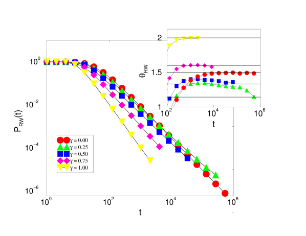
Figure 1: The survival probability of three random walkers. The inset shows the corresponding local exponents. The solid lines correspond to the analytic values given by $\theta_{RW}=2/(2-\gamma)$. The data are averaged over variable number of realizations ranging from $10^{9}$ for $\gamma=0$ to $2\times 10^{7}$ for $\gamma=0.5$. The initial distance between particles is $10$.

Figure 1 shows the survival probabilities obtained from simulations. $P_{\rm RW}(t)$ clearly decays as a power-law for large times. For $\gamma=0$ the survival exponent saturates to the asymptotic value $\theta_{RW}=3/2$ around $t\approx 10^{4}$ as shown in the inset, where the local survival exponent is presented. The exponent saturates also for $\gamma=0.75$ and $\gamma=1$. For $0<\gamma<0.75$ the survival exponent is slowly approaching the asymptotic value given by $\theta_{RW}=2/(2-\gamma)$. For $\gamma=0.75$ $r\approx 60$ at the time when the exponent saturates. This would correspond to $t_{\rm cr}\approx 2\times 10^{5}$ and $3\times 10^{12}$ for $\gamma=0.50$ and $0.25$, respectively. Thus we can not reach the asymptotic regime for $\gamma\lesssim 0.5$.

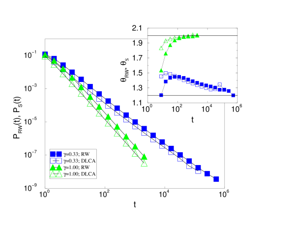
Figure 2: a) Comparison between the random walk and DLCA survival probabilities. b) The corresponding local exponents. The solid lines correspond to the analytic values given by $2/(2-\gamma)$. The RW simulations are averaged over $2.5\times 10^{10}$ ($\gamma=0.33$) and $2\times 10^{10}$ ($\gamma=1.00$) realizations with the initial distance between particles being 2. The DLCA simulations are averaged over $50000$ realizations on a system of size $55555$.

In Figure 2 the DLCA and RW survival probabilities are compared. The two behaviors agree except for a small difference between the amplitudes. The initial inter-particle distances are taken to be the same, in order the RW-picture to be as close to DLCA as possible. Notice the figure contains a case ($\gamma=0.33$) in which the asymptotic regime is not reached.

For $\gamma<0$ the survival probability decays stretched exponentially for both RW and DLCA systems (not shown). However, the stretching exponents differ from each other. This further supports the importance of fluctuations for $\gamma<0$. For RW survival we obtain $\beta_{\rm RW}\approx 0.33,0.31,0.25,$ and 0.19 for $\gamma=-6,-4,-2,$ and $-1$, respectively. For DLCA the numerics suggest an expression $\beta_{S}=2/3(1-2z)$. We also separately checked that the average size of the neighbors of unaggregated clusters in DLCA grows as $t^{z}$. Note, that $\lim_{\gamma\to-\infty}\beta_{S}=2/3$ and not a simple exponential ($\beta_{S}=1$) as one might expect based on the case of two immobile neighbors. It is also quite surprising, that the mean field approximation works better for a broad cluster size distribution ($\gamma\geq 0:f(x)\sim x^{-\tau}(x\to 0)$) than in the case, where the distribution is narrow around the mean ($\gamma<0:f(x)$ decays faster than any power law at both ends).

To summarize the results the survival probability decays as

$$P_{S}(t)\sim\begin{cases}\exp(-Ct^{\beta_{S}})&,\gamma<0\\ t^{-3/2}&,\gamma=0\\ t^{-2/(2-\gamma)}&,0<\gamma<2.\end{cases}$$ (4)

The survival exponent is discontinuous at $\gamma=0$, i.e., $3/2=\theta_{S}(0)>\theta_{S}(0^{+})=1$. This seems first counterintuitive since making some of the particles to diffuse faster helps the other to survive longer! This is the best since the surviving particle eventually “discovers” the optimal strategy [15] of remaining stationary. This is further confirmed by the fact that the probability of finding a site that has never been under any of the clusters decays as power-law with the exponent $2/(2-\gamma)$ for all $\gamma<2$ [13]. For $\gamma<0$ the surviving clusters no longer remain stationary.

The third exponent of interest in DLCA scaling is the decay exponent, $w$, which describes the decrease of the number of clusters of a fixed size $s$ as a function of time $n_{s}(t)\sim t^{-w}$. As the other exponents $z$ and $\tau$, it is expected to depend on $\gamma$. The three exponents are related by the scaling relation [16] $w=(2-\tau)z.$ Therefore dynamic scaling is fully characterized by any two of the exponents. Even on mean-field level (Smoluchowski’s equation) the only easy exponent is $z$ since it does not involve the full scaling function as in the case of and $\tau$ and $w$[7].

For $\gamma=0$ an exact solution of the cluster size distribution $n_{s}(t)$ is possible, with $w=3/2$ for any short-range correlated initial distribution $n_{s}(0)$ [11]. For a monodisperse initial condition, $n_{s}(0)=\delta_{1,s}$, the survival probability is simply $n_{1}(t)$, yielding the exponent $\theta_{S}(0)=3/2$. For $\gamma>0$ the dynamics of the clusters in the $s\ll S(t)$ part of the size distribution is dictated by collisions with larger, faster ones, that remove such small clusters from the tail. The mechanism by which clusters stay in the tail should be the same as for the survival problem. Thus for $0\leq\gamma<2$ one should have for the decay exponent $w=\theta_{S}=2/(2-\gamma)=2z$ together with the scaling relation

$$\theta_{S}=(2-\tau)z.$$ (5)

The numerically estimated values for the exponents fulfill Eq. 5 within the error bars for all values of the diffusion exponent $\gamma$ [12]. Hence, the polydispersity exponent is discontinuous at $\gamma=0$ since $\tau(0)=-1\neq 0=\tau(0^{+})$, similarly to some examples on the mean-field level [17]. It is also surprisingly enough independent of the value of $\gamma$.

Simulations confirm this although crossover effects make the analysis intractable near $\gamma=0$. Figure 3 shows the scaling plots for the cluster size distribution for various values of the diffusion exponent. The bigger the $\gamma$ is the faster the scaling function approaches a constant near $x=0$. For $\gamma\lesssim 0.5$ the times reached in simulations are too small to reveal the asymptotic scaling behavior. In this region also the measurements of $w$ from $n_{s}(t)\sim t^{-w}$ give information only on the crossover effects [18].

In summary, we have studied the survival of clusters in DLCA in one dimension. The decay of the initial state equals the density of clusters that stay intact by not aggregating with others. This can be analyzed on the mean-field level as the survival of a random walker bounded by two others with time-dependent diffusion coefficients. This maps to diffusion in a wedge with absorbing boundaries and time-dependent wedge angle. For $\gamma>0$ the surviving particles are such that they pick the strategy of staying immobile. The resulting survival exponent is non-monotonic and discontinuous at $\gamma=0$. Cluster survival determines the polydispersity exponent $\tau$ that characterizes the small cluster size tail. It is discontinuous and constant, $\tau=0$, for $0<\gamma<2$. For $\gamma<0$ the survival probability decays stretched exponentially, the fluctuations of the neighboring clusters determine the stretching exponent, and the mean-field RW-picture gives only a qualitative understanding of the survival.

Above one dimension the study of cluster survival will be both interesting and much less straightforward. A similar mean-field picture in terms of first-passage times of random walks is not directly applicable. For example, one lacks much of the theory needed to analyze the survival behavior of many interacting particles. We conclude with the conjecture that the solution of the survival problem is related to the cluster size distribution also in higher dimensions. There it should be possible to find experimental realizations, to study the survival phenomenon [19].

Acknowledgements - We thank Erik Aurell and Amit K. Chattopadhyay for discussions. This research has been supported by the Academy of Finland’s Center of Excellence program.

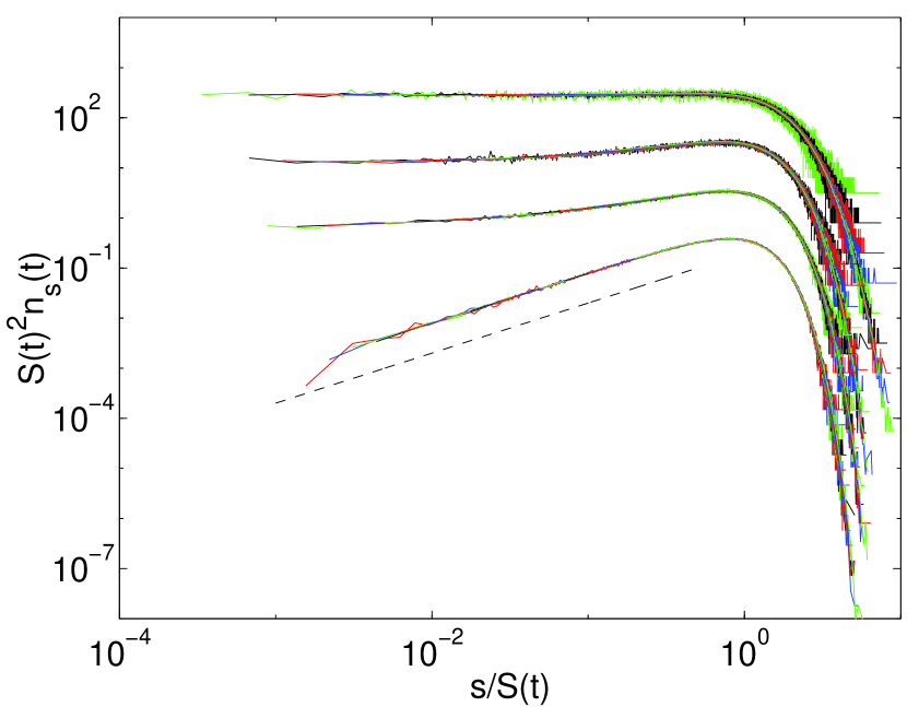
Figure 3: The scaling of the cluster size distributions for $\gamma=$ 0.00, 0.40, 0,57, and 1,00 (from bottom to top). Distributions are shown at times from $t=2^{3}$ to $2^{k_{\rm max}}$, where $k_{\rm max}=$ 17, 15, 14, and 11 for $\gamma=$ 0.00, 0.40, 0,57, and 1,00, respectively. The dashed line has a slope 1. The data are averaged over 50000 realizations on a system of size $55555$. The distributions (except the $\gamma=0$ distribution) have been shifted in the vertical direction for clarity.

References

- [1] See, for example, Kinetics of Aggregation and Gelation, edited by F. Family and D. P. Landau (North-Holland, Amsterdam, 1984).
- [2] S. Redner, A Guide to First-Passage Processes (Cambridge University Press, New York, 2001).
- [3] S. N. Majumdar, Curr. Sci. (India) 77, 370 (1999).
- [4] P. Meakin, Phys. Scripta 46, 295 (1992).
- [5] S. N. Majumdar, C. Sire, A. J. Bray, and S. J. Cornell, Phys. Rev. Lett. 77, 2867 (1996); B. Derrida, V. Hakim, and R. Zeitak, Phys. Rev. Lett. 77, 2871 (1996).
- [6] K. Kang, S. Redner, P. Meakin, and F. Leyvraz, Phys. Rev. A 33, 1171 (1986); S. Miyazima, P. Meakin, and F. Family, Phys. Rev. A 36, 1421 (1987).
- [7] P. G. J. van Dongen and M. H. Ernst, Phys. Rev. Lett. 54, 1396 (1985).
- [8] S. Cueille and C. Sire, Phys. Rev. E 55, 5465 (1997).
- [9] K. Kang and S. Redner, Phys. Rev. A 30, 2833 (1984).
- [10] M. E. Fisher, J. Stat. Phys. 34, 667 (1984).
- [11] J. L. Spouge, Phys. Rev. Lett. 60, 871 (1988).
- [12] E. K. O. Hellén, P. E. Salmi, and M. J. Alava, in preparation.
- [13] E. K. O. Hellén and M. J. Alava, in preparation.
- [14] B. Derrida and R. Zeitak, Phys. Rev. E 54, 2513 (1996).
- [15] S. Redner and P. L. Krapivsky, Am. J. Phys 67, 1277 (1999).
- [16] T. Vicsek and F. Family, Phys. Rev. Lett. 52, 1669 (1984).
- [17] P. G. J. van Dongen and M. H. Ernst, Phys. Rev. A 32, 670 (1985).
- [18] E. K. O. Hellén, T. P. Simula, and M. J. Alava, Phys. Rev. E 62, 4752 (2000).
- [19] For a particle tracking technique suitable perhaps for this purpose, see M.T. Valentine, P.D. Kaplan, D. Thota, J.C. Crocker, T. Gisler, R.K. Prud’homme, M. Beck, and D.A. Weitz, preprint, available from http://www.deas.harvard.edu/projects/weitzlab/.