[

Phase transition induced hydrodynamic instability and Langmuir-Blodgett Deposition

Abstract

We propose a model to understand periodic oscillations relevant to the origin of mesoscopic channels formed during a Langmuir-Blodgett deposition observed in recent experiments {M. Gleiche, L.F. Chi, and H. Fuchs, Nature 403, 173 (2000)}. We numerically study one-dimensional flow of a van der Waals fluid near its discontinuous liquid-gas transition and find that steady-state flow becomes unstable in the vicinity of the phase transition. Instabilities leading to complex periodic density-oscillations are demonstrated at some suitably chosen sets of parameters.

]

Studies of pattern formation in non-equilibrium systems have attracted considerable attention due to their relevance in understanding fundamental physics and the potential for applications in a wide range of emerging technologies. The spontaneously formed patterns can be converted into functional structures when the pattern forming mechanism is properly controlled and designed. Typically, this class of pattern formation involves systems flowing at conditions around which the properties undergo dramatic changes. The patterns are a result of the occurrence and propagation of a phase transition or chemical reaction, the Belousov-Zhabotinsky reaction [1] and capillary flow of molten polymer [2] being two examples. One of the key issues to be understood in these systems is the nontrivial coupling between the system specific ‘phase transition’ and the hydrodynamics.

Our work has been motivated by recent experiments that have demonstrated the formation of macroscopic arrays of submicron-sized channels during a Langmuir-Blodgett deposition [3]. Mechanisms based on stick-slip conditions have been proposed to describe the phenomenon [3, 4]. However, in this Letter, we propose a different scenario in which density oscillations occur in the flow of a single-component fluid at conditions tuned appropriately near its discontinuous liquid-gas phase transition. The system fails to support steady-state flow at these conditions due to the absence of a mechanically stable uniform state in a certain density interval. The instability leads to periodic oscillations in density or alternating appearance of liquid and gaseous phases in the system. The oscillations can be potentially useful in producing large arrays of periodic structures and we propose this as a possible mechanism for the experiments [3] mentioned above. The problem of fluid flow in the vicinity of a phase transition has been widely studied [5]. A closely related subject on propagation of the phase transition front has also been investigated in detail[6]. However, we are not aware of any previous work on unstable one-dimensional flow of a single-component fluid that leads to periodic density-oscillations of this nature. A realization of such a system is a fluid flowing in a narrow channel, or higher dimensional flow in which spatial variations of the system properties are suppressed in the direction transverse to the fluid velocity. The flow of surfactant molecules in a typical Langmuir-Blodgett deposition is an example in two-dimensions [7, 8].

Our analysis begins with the standard hydrodynamics at constant temperature consisting of the continuity equation and the Navier-Stokes equation for a one-dimensional flow of compressible fluid as follows:

$$\frac{\partial\rho}{\partial t}+\frac{\partial\rho v}{\partial x} = 0,$$ (1)

$$\rho\left(\frac{\partial v}{\partial t}+v\frac{\partial v}{\partial x}\right) = -\frac{\partial P}{\partial x}+\eta\frac{\partial v^{2}}{\partial x^{2}},$$ (2)

where $\rho$ is the density, $v$ is the velocity and $\eta$ is the viscosity. The main feature of the system is contained in the quantity $P$, the local pressure of the inhomogeneous fluid. It is expressed as [9]

$$P=\rho\frac{\delta\Psi[\rho]}{\delta\rho}-\psi(\rho)+\frac{\kappa}{2}\left(\frac{\partial\rho}{\partial x}\right)^{2},$$ (3)

which is also the equation of state of the fluid. Here, the quantity $\Psi[\rho]$ denotes the Helmholtz free energy density for an inhomogeneous fluid [9] given by,

$$\Psi[\rho]=\int\left\{\frac{\kappa}{2}\left(\frac{\partial\rho}{\partial x}\right)^{2}+\psi(\rho)\right\}dx,$$ (4)

where $\psi(\rho)$ is the Helmholtz free energy density of the homogeneous system and $\kappa$ is a phenomenological constant associated to the gradient term with a meaning that is specific to the particular system chosen. For a van der Waals (vdW) fluid, the Helmholtz free energy density of a uniform system is given by

$$\psi(\rho)=8\rho T\ln\frac{\rho}{3-\rho}-3\rho^{2},$$ (5)

where $T$ is the temperature and $\kappa$ is proportional to the surface tension of the liquid-gas interface. The reason for choosing a vdW fluid for our investigation is that it is one of the simplest descriptions that includes a discontinuous liquid-gas transition and a region in the $P-\rho$ plane where the uniform fluid is unstable (negative compressibility) below the critical temperature $T_{c}\equiv 1$. We note that the quantities $P$, $\rho$ and $T$ in Eqs. (3) and (5) have been normalized by their respective values at the critical point for convenience. We also remark that the fluid is maintained at thermal equilibrium at all times, that is, Eq. (3) always holds. It is the mechanical stability that is being investigated here.

FIG. 1.: Schematics of the flow configurations. The quantities $v_{i}$ and $\rho_{i}$ are, respectively, the inlet velocity and density while the outlet velocity is denoted by $v_{o}$.

A numerical algorithm has been developed to solve Eqs. (1) and (2) using the forward-time-centered-space approach described in Ref. [10]. We will restrict ourselves to a special case depicted in Fig. 1: a flow in the region $x\in[0,L]$ subject to the following set of boundary conditions

$$v(x<0,\;t) = v_{0},$$ (6)

$$v(x>L,\;t) = v_{L},$$ (7)

$$\rho(x<0,\;t) = \rho_{0},$$ (8)

$$\rho(x>L,\;t) = \rho(L,\;t).$$ (9)

The fluid velocity has been arbitrarily chosen so that it flows from left to right. The positions $x=0$ and $x=L$ correspond to, respectively, the inlet and the outlet. The quantities $v_{0}$ and $v_{L}$ are, respectively, the velocities at the inlet and the outlet. The density at the inlet is kept at $\rho_{0}$. This set of boundary conditions describes a situation where both the fluid density and velocity are kept fixed at the inlet, and the fluid density at the outlet is allowed to vary with time while keeping the velocity constant. Under this special circumstance, the instability of the flow is necessarily reflected in the time dependence of the density at the outlet and we systematically analyze $\rho(L,\;t)$. We remark that there are a total of six parameters involved, namely, $v_{0}$, $v_{L}$, $\rho_{0}$, $T$, $\eta$ and $\kappa$. In general, the solutions to Eqs. (1) and (2)  are complex and possess many degrees of freedom. Here, we will focus our discussions on the results for a restricted sets of parameters.

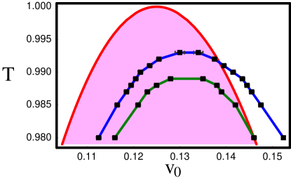
FIG. 2.: The comparison between the computed instability boundary (blue) and that estimated from the spinodal boundary (red) for $\rho_{0}=0.8$, $v_{L}=0.1$, $\eta=0.01$ and $\kappa=0.0001$. Also shown in green is the boundary between the simple and complex oscillatory behavior in the unstable region.

When the density at the inlet $\rho_{0}$ and the velocity at the outlet $v_{L}$ are kept fixed, the behavior of $\rho(L,\;t)$ as $v_{0}$ varies can be understood intuitively as follows: if one insists on a steady-state flow, the density at the outlet $\rho(L,\;t)$ has to be

$$\rho(L,\;t)=\frac{v_{0}\rho_{0}}{v_{L}}.$$ (10)

Since Eq. (3), the equation of state of the fluid, allows for a region where the compressibility is negative (spinodal region), mechanical instability is thus inevitable if $v_{0}\rho_{0}/v_{L}$ falls within the spinodal region. A rough estimate of the stability boundary, assuming the system is uniform, is given by $v_{L}$’s for which $\rho(L,\;t)$ coincides with the spinodal boundary (i.e., state of the fluid where compressibility diverges). Our numerical results indeed show that the steady state solution fails to be stable in some regions of the parameter space, restricted to the $v_{0}-T$ plane in this work. The instability region in the $v_{0}-T$ plane has been identified numerically. Figure 2 compares the computed stability boundary (blue) and that estimated from the spinodal boundary (red). The discrepancy between the estimates and the numerical results is a consequence of the shift in the spinodal region due to the flow-induced density gradient and is evident from Eq. (3).

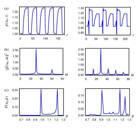
FIG. 3.: Plots of (a) $\rho(L,\;t)$, (b) $|\tilde{\rho}(L,\;\omega)|^{2}$ and (c) $P(L,\;\rho)$ for the case of simple oscillation at $v_{0}$=0.142 on the left panel, and for the case of complex oscillations at $v_{0}=0.136$ on the right. The other parameters are set to $v_{L}=0.1$, $\rho_{0}=0.8$, $T=0.987$, $\eta=0.01$, and $\kappa=0.0001$.

Our results further show that the instability leads to oscillatory behavior in $\rho(L,\;t)$, the density at the outlet. The density-oscillations have been classified into two classes: a ‘simple’ oscillation in which $\rho(L,\;t)$ oscillates between two densities, and a more ‘complex’ oscillation where $\rho(L,\;t)$ cycles among three or more densities. The left panels of Fig. 3 illustrate the behavior of a simple density-oscillation whereas the right panels show a case of complex oscillations. Figure 3(a) displays plots of $\rho(L,\;t)$, showing the time evolution of the density at the outlet. The plots of spectral density $|\tilde{\rho}(L,\;\omega)|^{2}$ are shown in Fig. 3(b). A primary peak accompanied by its weaker harmonics is shown on the left panel; a more complicated structure exists on the right panel. Furthermore, the number of densities among which $\rho(L,\;t)$ cycles can be picked out by evaluating the density distribution function $P(L,\;\rho)\equiv{\cal N}^{-1}\int\delta[\rho(L,\;t)-\rho]dt$ where ${\cal N}\equiv\int P(L,\;\rho)d\rho$ is the normalization constant. Figure 3(c) displays $P(L,\;\rho)$ with two peaks on the left and three on the right. The green curve in Fig. 2 is the boundary in the $v_{0}-T$ plane separating the region of simple and complex oscillations. Simple oscillations occur in the region between the blue and the green curves, while complex oscillations are found under the green curve.

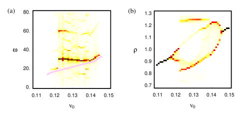
FIG. 4.: Density plots of (a) $|\tilde{\rho}(L,\;\omega)|^{2}$ as a function of $\omega$ and $v_{0}$, and (b) $P(L,\;\rho)$ as a function of $\rho$ and $v_{0}$. The pink curve in (a) is a guide-to-eye for the trend of the principal peak in the region of simple oscillations. Deviation from this curve indicates the region of complex oscillation $v_{0}\in(0.123,0.139)$. This region can be clearly identified in (b) by the onset of additional peaks. The parameters used are $\rho_{0}=0.8$, $v_{L}=0.1$, $T=0.987$, $\eta=0.01$ and $\kappa=0.0001$.

Figure 4(a) is a density plot of $|\tilde{\rho}(L,\;\omega)|^{2}$ versus $v_{0}$ and $\omega$, and Fig. 4(b) is a density plot of $P(L,\;\rho)$ as a function of $v_{0}$ and $\rho$, showing the dependence of these functions on the inlet velocity $v_{0}$, while keeping other parameters fixed. Higher intensity is represented by darker colors in the density plots, highlighting the peaks of the functions. The appearance of peaks at nonzero frequency in $|\rho(L,\;\omega)|^{2}$, and the multi-peak structures in $P(L,\;\rho)$ reflect the unstable region in $v_{0}$ [$v_{0}\in(0.119,0.146)$] at $T=0.987$. The region of complex oscillation at $T=0.987$ with $v_{0}\in(0.123,0.139)$ can be identified as the deviation from the simple structure of a single principal peak in $|\tilde{\rho}(L,\;\omega)|^{2}$ [the trend of the principal peak is shown by the pink curve in Fig. 4(a)], and the onset of additional peaks in $P(L,\;\rho)$ other than the two expected for simple oscillations.

The scenario described by Eqs. (1) and (2) with boundary conditions given by Eqs. (6)-(9) can be related to the flow of a Langmuir monolayer (a single molecular layer of insoluble surfactant molecules spread at the air/water interface) during a Langmuir-Blodgett deposition. In a Langmuir-Blodgett deposition, a substrate is withdrawn from or dipped into the water transferring the surfactant molecules onto the substrate at the contact line. The surfactant molecules are removed at the substrate withdrawal speed at the contact line. The boundary conditions at the outlet, Eqs. (7) and (9), are explicitly realized at the contact line if the transfer ratio is unity at all times. Although the correspondence between the inlet boundary conditions and the actual experiments is not completely clear, Eqs. (6) and (8) are reasonable for an appropriately chosen $L$. A sensible estimate of the inlet-outlet separation $L$ for the Langmuir-Blodgett deposition would be the meniscus height at the contact line, which is $\sim 10^{-3}$m. Hence, the specific choice of boundary conditions, Eqs. (6)-(9), can be realistic. Despite the attempt to associate the proposed scenario to the actual experiment, the model is far from a complete description of the system. Many details relevant to the Langmuir monolayer such as long-range dipolar interactions between the surfactant molecules, surfactant-water interactions [8], water flow near the contact line [7, 11], elasticity of the monolayer [12], are not taken into account. Nevertheless, the key emphasis is to point out that a discontinuous phase transition has been shown to lead to simple period density-oscillations which provide a possible mechanism for the formation of macroscopic arrays of mesoscopic structures.

In summary, we have demonstrated numerically that a one-dimensional flow of a van der Waals fluid near its discontinuous liquid-gas transition exhibits a hydrodynamic instability leading to periodic, classified as simple and complex, oscillatory behavior. We highlight the key point of our analysis: the instability in this simple system arises because of the inability to support a steady-state solution when enforcing the continuity equation in the vicinity of a discontinuous transition. Hence, this oscillatory behavior is not restricted to van der Waals fluids and could be observed in other kinds of systems (with well prescribed equation of state) that possess similar features. We have attempted to relate this one-dimensional model to Langmuir-Blodgett deposition where the boundary conditions can be physically realized. This simple model provides us with a route to periodic oscillatory behavior that has been observed [3]. We note that the region in the parameter space where simple oscillations occur is limited. This is a possible explanation for the difficulty in finding the periodic oscillations and their sensitivity to experimental conditions, such as pressure and temperature. Estimates for the period and the interval of each of the phases, within the framework of this model, require a knowledge of the continuation of the equation of state into the metastable regime and the spinodals.

We thank Dr. Hans Riegler, Dr. Jack F. Douglas, Professor Boris Malomed, Professor Rashmi Desai and Professor Yulii Shikhmurzaev for many interesting discussions. One of us (KL) acknowledges a Director’s Fellowship at Los Alamos National Laboratory. This work was supported by the US Department of energy.

REFERENCES

- [1] A.G. Merzhanov and E.N. Rumanov, Rev. Mod. Phys. 71, 1173 (1999).
- [2] J.D. Shore, D. Ronis, L. Piché, and M. Grant, Phys. Rev. Lett. 77, 655 (1996).
- [3] M. Gleiche, L.F. Chi, and H. Fuchs, Nature 403, 173 (2000); K. Spratte, L.F. Chi, and H. Riegler, Europhys. Lett. 25, 211 (1994); H. Riegler and K. Spratte, Thin Solid Films 210/211, 9 (1992).
- [4] L.G.T. Eriksson, P.M. Claesson, S. Ohnishi, and M. Hato, Thin Solid Films 300, 240 (1997).
- [5] A. Onuki, J. Phys.: Condens. Matter 9, 6119 (1997).
- [6] O. Inomoto, S. Kai, and B.A. Malomed, Phys. Rev. Lett. 85, 310 (2000)
- [7] J.G. Petrov, H. Kuhn, and D. Möbius, J. Colloid Interface Sci. 73, 66 (1980).
- [8] D.K. Schwartz, C.M. Knobler, and R. Bruinsma, Phys. Rev. Letts. 73, 2841 (1994); H.A. Stone, Phys. Fluids 7, 2931 (1995).
- [9] R. Evans, Advances in Physics 28, 143 (1979).
- [10] W.H. Press, S.A. Teukolsky, W.T. Vetterling, and B.P. Flannery, Numerical Recipes in C (Cambridge University Press, Cambridge, U.K. 1992).
- [11] Y.D. Shikhmurzaev, Int. J. Multiphase Flow 19, 589 (1993); T.D. Blake, M. Bracke, and Y.D. Shikhmurzaev, Phys. Fluids 11, 1995 (1999).
- [12] J.F. Douglas, private communications.