Complementary approaches to the
ab initio calculation of melting properties

Abstract

Several research groups have recently reported ab initio calculations of the melting properties of metals based on density functional theory, but there have been unexpectedly large disagreements between results obtained by different approaches. We analyze the relations between the two main approaches, based on calculation of the free energies of solid and liquid and on direct simulation of the two coexisting phases. Although both approaches rely on the use of classical reference systems consisting of parameterized empirical interaction models, we point out that in the free energy approach the final results are independent of the reference system, whereas in the current form of the coexistence approach they depend on it. We present a scheme for correcting the predictions of the coexistence approach for differences between the reference and ab initio systems. To illustrate the practical operation of the scheme, we present calculations of the high-pressure melting properties of iron using the corrected coexistence approach, which agree closely with earlier results from the free energy approach. A quantitative assessment is also given of finite-size errors, which we show can be reduced to a negligible size.

1 Introduction

The study of solid-liquid equilibrium by computer simulation has a long history, going back to the classic work of Alder and Wainwright [1] on the hard-sphere system in the 1950’s. Many techniques have been used to determine the pressure-temperature relation at equilibrium and other melting properties, such as the volume and entropy of fusion. In the last few years, there has been an upsurge of interest in the accurate ab initio treatment of the melting properties of real materials [2, 3, 4, 5, 6, 7, 8], which has focused attention again on the techniques used to locate the melting transition. Recent ab initio work has been based on two main approaches. The first locates the melting transition by requiring equality of the Gibbs free energies, which are calculated ab initio for liquid and solid [2, 3, 4, 5, 6]; we call this the ‘free energy’ approach. The second proceeds by fitting a potential model to ab initio calculations and using this to simulate a system containing liquid and solid in coexistence [7, 8, 9]; we call this the ‘coexistence’ approach. If appropriate measures are taken, the two approaches should clearly give the same results. The purpose of this paper is to analyze the relation between the two approaches and to propose what these ‘appropriate measures’ should be. We illustrate our analysis by presenting ab initio calculations on the high-pressure melting of iron performed using the coexistence approach, which we compare with earlier free-energy results from the same ab initio technique [4, 5]. We shall show that, once the necessary corrections have been applied, the two approaches yield the same results.

The free-energy approach has been well established for many years for calculations based on classical interaction models (see e.g. Refs. [10, 11, 12]). Typically the procedure for the solid has been to start from the harmonic approximation at low temperatures; the free energy of the high-temperature anharmonic system is then obtained by using the Gibbs-Helmholtz relation to integrate the internal energy given by molecular dynamics (MD) simulation [10, 11]. Alternatively, the anharmonic free energy has sometimes been obtained by thermodynamic integration starting from a reference model such as the Einstein solid [12]. For the liquid, a common procedure has been to obtain the free energy at one thermodynamic state from the work done in reversible expansion [10, 12] to low density or heating to high temperature. The Gibbs-Helmholtz relation is then used to obtain the free energy at other states. We also mention an important alternative approach, known as ‘Gibbs-Duhem’ integration, which allows the boundary between coexisting phases to be directly mapped out [13, 14].

In early work, the interaction models were parameterized by fitting to experimental data, but recent years have seen a major shift towards the calculation of melting properties [2, 3, 4, 5, 6, 7, 8] from ab initio methods based on density-functional theory (DFT) [15]. In DFT, the total energy function of a system is determined by the approximation used for exchange-correlation energy $E_{\rm xc}$. An important ambition then follows: the determination of melting properties with no statistical-mechanical or other approximations except those inherent in $E_{\rm xc}$ itself. This raises major new issues, because it is extremely costly to perform ab initio MD (AIMD) simulations on large systems long enough to reduce statistical errors to an acceptable level. The cost is particularly great for crystals, since extensive electronic $k$-point sampling may be needed. Long accepted methods like reversible expansion to low density are impracticable with AIMD. Instead, it is essential to use empirical interaction models that closely mimic the DFT system. The usual techniques are then employed to treat these models, and in some ab initio work thermodynamic integration is used to obtain the free energy difference between the model and DFT systems [2, 3, 4, 5, 6]. In parallel with these developments, the advantages of avoiding intricate free-energy calculations by using the coexistence approach have made this route popular [7, 8, 9]. Again, the simulations must be based on empirical models matched to DFT data.

The present work was stimulated by recent reports of ab initio or nearly ab initio calculations on the melting of a number of materials, including Si [2], Al [3, 6], Cu [16] and Fe [4, 5, 7, 8]. Our own work on Al [3, 6] and Fe [4, 5] was based on the free-energy approach, which used an inverse-power reference model, with thermodynamic integration to calculate the difference between the ab initio and reference free energies. A major effort was made to ensure that finite-size and other systematic errors were reduced to an almost negligible level. The other ab initio work on Fe, by two independent groups, used the coexistence approach [7, 8]. The results for the melting curve differed substantially from each other and from our results, and we urgently need to understand the reasons for the disagreements. We aim to shed light on possible reasons here.

We shall explore a number of technical issues. The first concerns the correction of the coexistence method for errors due to the difference between the ab initio system and the empirical model that mimics it. A second issue is the fitting of models to ab initio data. We have already discussed this in depth for the free-energy approach, so here we focus mainly on coexistence. We want to study what physical quantities should be fitted, and how to tell if the fit is good enough. A third important issue concerns finite-size errors, which arise mainly from the limited system sizes that can be handled ab initio. It has been claimed [16] that the coexistence approach suffers less from size errors than the free-energy approach. We shall demonstrate that in fact this type of error affects both approaches in essentially the same way. One thing we shall not do is to pass judgment on which method is ‘better’, since we shall argue that the answer depends on what one wishes to achieve, and that both approaches are vital. However, we shall comment on the strengths and weaknesses of both.

In the next Section, we define the problem, summarize briefly the free-energy and coexistence approaches as they have been applied in practical ab initio calculations, analyze the corrections that need to be applied in the two approaches, and discuss size errors. Section 3 then presents our new calculations on the high-pressure melting properties of Fe using the coexistence approach. We shall compare with our earlier free-energy results and show the practical necessity of the corrections outlined in Sec. 2. The final Section gives further discussion and summarizes our conclusions.

2 Theory of the two approaches

2.1 Definition of the problem

We start by defining the problem to be addressed. At a given pressure $p$, two phases are in thermodynamic equilibrium when their Gibbs free energies $G(p,T)$ are equal. We regard $G$ as derived by the relation $G=F+pV$ from the Helmholtz free energy $F(V,T)$. The ab initio value of $F$ at any volume and temperature, denoted by $F_{\rm AI}(V,T)$, is given in classical statistical mechanics by:

$$F_{\rm AI}(V,T)=-k_{\rm B}T\ln\left\{\frac{1}{N!\Lambda^{3N}}\int d{\bf r}_{1}\ldots d{\bf r}_{N}\,e^{-\beta U_{\rm AI}({\bf r}_{1},\ldots{\bf r}_{N})}\right\}\;,$$ (1)

where $U_{\rm AI}({\bf r}_{1},\ldots{\bf r}_{N})$ is the ab initio total energy as a function of the positions ${\bf r}_{1},\ldots{\bf r}_{N}$ of the $N$ nuclei, which range over the volume $V$ of the cell containing the system. For the purpose of treating phase equilibria, we need the free energy per atom $F_{\rm AI}/N$ in the thermodynamic limit $N\rightarrow\infty$, $V\rightarrow\infty$ at constant number density $N/V$.

Even though the coexistence approach does not work directly with free energies, we shall show later that the errors that need to be overcome in this approach, as well as in the free-energy approach, can be formulated as free-energy errors. But the errors in calculating $F_{\rm AI}$ are of two kinds: electronic-structure errors, i.e. imperfections in the calculation of the ab initio total energy $U_{\rm AI}$ at each set of nuclear positions; and statistical-mechanical errors, i.e. errors in calculating $F_{\rm AI}$ from the given $U_{\rm AI}$, and in taking the thermodynamic limit.

For the purposes of this work, electronic-structure errors are irrelevant: our sole concern is the treatment of phase equilibrium using some given algorithm for computing $U_{\rm AI}$. The ‘free energy’ and ‘coexistence’ routes differ only in the way they address the statistical mechanics. Our problem is therefore to assess and compare the ways that the two approaches control the purely statistical-mechanical errors. When we come to the practical calculations in Sec. 3, we shall compare the results of the two approaches applied using exactly the same algorithm for $U_{\rm AI}$.

2.2 The free-energy approach

In the free-energy approach [2, 4, 5, 17], we use a reference system with total energy function $U_{\rm ref}({\bf r}_{1},\ldots{\bf r}_{N})$, whose solid and liquid free energies $F_{\rm ref}$ are calculated for very large systems, so that finite-size errors are negligible. Then the only demanding problem is the calculation of the difference $\Delta F\equiv F_{\rm AI}-F_{\rm ref}$, which is accomplished by thermodynamic integration [18]:

$$\Delta F=\int_{0}^{1}\langle\Delta U\rangle_{\lambda}\,d\lambda\;,$$ (2)

where $\Delta U\equiv U_{\rm AI}-U_{\rm ref}$, and the thermal average $\langle\,\cdot\,\rangle_{\lambda}$ is taken in the ensemble generated by the total-energy function $U_{\lambda}\equiv(1-\lambda)U_{\rm ref}+\lambda U_{\rm AI}$. In practice, $\langle\Delta U\rangle_{\lambda}$ is computed as a time average in an AIMD simulation whose dynamics is governed by $U_{\lambda}$. The main kinds of error are: statistical errors in the evaluation of $\langle\Delta U\rangle_{\lambda}$; integration errors due to inadequate numbers of $\lambda$ points; and finite-size errors. In the systems studied so far by this approach, all these errors can be brought under tight control.

It is a crucial feature of this approach that $F_{\rm AI}$, calculated as $F_{\rm ref}+\Delta F$, does not depend on the choice of reference system, provided all technical tolerances are set so as to suppress the errors we have just mentioned. However, for reasons expounded in detail elsewhere [4, 5, 6], the choice of $U_{\rm ref}$ has a major influence on the overall computational effort, which is minimized by reducing as much as possible the strength of the fluctuations $\left\langle\delta\Delta U^{2}\right\rangle_{\lambda}/N$, where $\delta\Delta U\equiv\Delta U-\langle\Delta U\rangle_{\lambda}$. In particular, minimization of this fluctuation strength is important in ensuring that $F_{\rm ref}$ accounts for almost all the free energy, so that size errors in the small residue $\Delta F$ are negligible. This can be achieved by using a parameterized reference model whose parameters are adjusted so as to minimize $\langle\delta\Delta U^{2}\rangle_{\lambda}/N$, as in our work on the melting of Fe. In this approach, it is an advantage that different reference systems can be used for solid and liquid, since for many materials it may be difficult to create $U_{\rm ref}$ functions that mimic $U_{\rm AI}$ with high precision in both phases.

2.3 The coexistence approach

The coexistence approach is also based on a reference model that mimics the ab initio system. (This model is sometimes called by names such as ‘optimised potential model’ [7, 19], but here we give it the same name as in the free-energy approach.) Various ways have been used to fit the reference model to the ab initio system. Since it will be relevant later, we note that recent coexistence work on Fe has used the ‘force-matching’ procedure of Ercolessi and Adams [19], in which the reference parameters are adjusted so that the ab initio atomic forces are reproduced as well as possible for representative sets of atomic positions.

There are also several ways of using the reference model to simulate coexisting phases, and hence to determine the phase boundary between them. In the work of Morris et al. [9], coexisting solid and liquid Al were simulated with the total number of atoms $N$, volume $V$ and internal energy $E$ fixed. They showed that, provided $V$ and $E$ are appropriately chosen, the two phases coexist stably over long periods of time, and the average pressure $p$ and temperature $T$ in the system give a point on the melting curve. The underlying concept is that the mean volume per atom $\bar{v}\equiv V/N$ is given by:

$$\bar{v}=(1-x_{l})v_{s}(p)+x_{l}v_{l}(p)\;,$$ (3)

where $x_{l}$ is the fraction of the atoms in the liquid phase, with $v_{s}(p)$ and $v_{l}(p)$ the volumes per atom in the coexisting solid and liquid as a function of pressure. For fixed $\bar{v}$, the pressure $p$ traverses a certain range as $x_{l}$ goes from 0 to 1. As $x_{l}$ varies in this way, the mean internal energy per atom $\bar{e}\equiv(1-x_{l})e_{s}(p)+x_{l}e_{l}(p)$ also traverses some range (here, $e_{s}(p)$ and $e_{l}(p)$ are the internal energies per atom in the two phases). Provided $\bar{e}$ lies in this range for the given $\bar{v}$, the simulation will yield stably coexisting solid and liquid. An alternative procedure would be to simulate at constant $(N,V,T)$. Then coexistence will be achieved for a given $\bar{v}$ provided $T$ is chosen so that the corresponding $p$ on the melting line curve falls in the range specified by Eq. (3). Yet another approach was used in the work of Laio et al. [7] on the high-pressure melting of Fe; this used constant-stress simulations, with enthalpy almost exactly conserved. The approach of Belonoshko et al. [8] is different again. Here, the $(N,p,T)$ ensemble is used. The system initially contains coexisting solid and liquid, but since $p$ and $T$ generally do not lie on the melting line, the system ultimately becomes entirely solid or liquid. This approach does not directly yield points on the melting curve, but instead provides upper or lower bounds, so that a series of simulations is needed to locate the transition point. Whichever scheme is used, some way is needed of monitoring which phases are present. In the $(N,V,E)$ method of Morris et al. [9], graphical inspection of particle positions appears to have been used, supplemented by calculating of radial distribution functions to confirm the crystal structure of the solid. In the $(N,p,T)$ method of Belonoshko et al. [8], the primary diagnostic is the discontinuity of volume as the system transforms from solid to liquid.

The coexistence calculations presented here on the high-pressure melting of Fe employ the $(N,V,E)$ method applied to reference systems consisting of the ‘embedded-atom model’ [20] fitted to ab initio data. For geophysical reasons, we are interested in pressures near that at the boundary between the Earth’s inner and outer cores, namely 330 GPa [21]. In this pressure region, the most stable crystal structure just below the melting curve is believed to be hexagonal close packed (h.c.p.) [22, 23], and we assume here that melting occurs from this phase. We start with a simulation cell containing only the h.c.p. solid, with the basal plane parallel to one face of the cell, and the system is allowed to thermalize at a temperature where coexistence is expected. At some instant of time, the simulation is stopped, and the atoms in one half of the system are held fixed; the boundary between the two halves is taken parallel to the h.c.p. basal plane. The atoms in the other half are raised to a very high temperature, and dynamical evolution of these atoms is allowed to proceed so that melting occurs. With this half of the system molten, its temperature is now reduced to the original value, the atoms in the other half still being fixed. Finally, the atoms in the fixed half are given thermal velocities and released, and the whole system is allowed to evolve freely. The system is monitored by calculation of the average number density in slices of the cell taken parallel to the boundary between solid and liquid. As we shall show, the density in the solid part is a periodic function of slice number, while in the liquid it fluctuates rather weakly about its average value. The total energy, temperature and pressure are, of course, monitored throughout the simulation. A feature of the $(N,V,E)$ method is that at equilibrium the stress in the solid phase will generally not be hydrostatic, and manual adjustment of the cell parameters is needed to achieve hydrostatic stress. We shall show in Sec. 3 that this does not present a problem.

2.4 Correcting the coexistence approach

Both the free-energy and the coexistence approaches are subject to errors, which need to be assessed and corrected for. It may be too costly to perform all the ab initio calculations with the precision needed to obtain accurate melting properties, so that there are errors due to inadequate $k$-point sampling, incompleteness of the basis set, or other approximations. In the coexistence approach, inevitable differences between the reference and ab initio total energies will create errors in the melting properties, which need to be evaluated. The correction of errors in the free-energy approach has been extensively discussed elsewhere [5, 17], so our main concern here is correction of the coexistence approach.

Assuming the ab initio energy is calculated with adequate precision, the main error comes from differences between $U_{\rm AI}$ and $U_{\rm ref}$. The key question posed here is therefore: how are predicted melting properties changed by small changes in the total energy function? (System-size errors will be discussed separately later.) Related questions have been discussed before (see e.g. Ref. [14]), so we give only a brief summary of the main points.

The difference $U_{\rm AI}-U_{\rm ref}$ is denoted by $\Delta U$, as in the free-energy approach. The change of any quantity resulting from the replacement of $U_{\rm ref}$ by $U_{\rm AI}$ will also be indicated by $\Delta$; for example, the shift of melting temperature at a given pressure is called $\Delta T_{\rm m}$. The melting temperature is shifted because the liquid and solid Gibbs free energies $G^{l}(p,T)$ and $G^{s}(p,T)$, and hence their difference $G^{ls}(p,T)\equiv G^{l}(p,T)-G^{s}(p,T)$, are shifted. Working at the given pressure, we take the variable $p$ as read and express the ab initio value of $G^{ls}$ as:

$$G_{\rm AI}^{ls}(T)=G_{\rm ref}^{ls}+\zeta\Delta G^{ls}(T)\;,$$ (4)

where the parameter $\zeta$ is introduced so that the reference melting temperature $T_{\rm m}^{\rm ref}$ can be written as a power series:

$$T_{\rm m}^{\rm AI}=T_{\rm m}^{\rm ref}+\zeta T_{\rm m}^{\prime}+\zeta^{2}T_{\rm m}^{\prime\prime}+\ldots\;.$$ (5)

Since the Gibbs free energies are equal in the two phases, this $T_{\rm m}^{\rm AI}$ is the solution of $G_{\rm AI}^{ls}(T)=0$, which is:

$$G_{\rm ref}^{ls}\left(T_{\rm m}^{\rm ref}+\zeta T_{\rm m}^{\prime}+\zeta^{2}T_{\rm m}^{\prime\prime}\ldots\right)+\zeta\Delta G^{ls}\left(T_{\rm m}^{\rm ref}+\zeta T_{\rm m}^{\prime}+\zeta^{2}T_{\rm m}^{\prime\prime}+\ldots\right)=0\;.$$ (6)

Expanding in powers of $\zeta$ and equating powers, one obtains formulas for $T_{\rm m}^{\prime}$, $T_{\rm m}^{\prime\prime}$, etc:

$$T_{\rm m}^{\prime} = \Delta G^{ls}\left(T_{\rm m}^{\rm ref}\right)\left/S_{\rm ref}^{ls}\right.$$

$$T_{\rm m}^{\prime\prime}/T_{\rm m}^{\prime} = -\frac{1}{S_{\rm ref}^{ls}}\left[T_{\rm m}^{\prime}C_{p,{\rm ref}}^{ls}/2T_{\rm m}^{\rm ref}+\Delta S^{ls}\right]\;,$$ (7)

where $S_{\rm ref}^{ls}\equiv S_{\rm ref}^{l}-S_{\rm ref}^{s}$ is the reference entropy of fusion, $C_{p,{\rm ref}}^{ls}\equiv C_{p,{\rm ref}}^{l}-C_{p,{\rm ref}}^{s}$ is the liquid-solid difference of the constant-pressure specific heats, and $\Delta S^{ls}$ is the shift of the entropy of fusion. We note particularly the implication of the formula for $T_{\rm m}^{\prime}$. Since entropies of fusion are on the order of $k_{\rm B}$ per atom, then a difference $\Delta G^{ls}$ of 10 meV/atom implies a shift of melting temperature of ca. 100 K, so that substantial errors will need to be corrected for unless the reference total energy function matches the ab initio one very precisely. Although we have included a formula for $T_{\rm m}^{\prime\prime}$, it seems unlikely that this will be used in practice, except perhaps for a rough estimate of $T_{\rm m}^{\prime\prime}/T_{\rm m}^{\prime}$, since $\Delta S^{ls}$ would be difficult to compute without rather extensive free-energy calculations.

If simulations are done in the isothermal-isobaric ensemble, then for closely matching $U_{\rm AI}$ and $U_{\rm ref}$, with small fluctuations of $\Delta U$, the Gibbs free energy shifts $\Delta G^{l}$ and $\Delta G^{s}$ can be evaluated using the well-known expansion:

$$\Delta G=\langle\Delta U\rangle_{\rm ref}-\frac{1}{2}\beta\langle\delta\Delta U^{2}\rangle_{\rm ref}+\ldots\;,$$ (8)

where $\delta\Delta U\equiv\Delta U-\langle\Delta U\rangle_{\rm ref}$, and the averages are taken in the reference ensemble. The ab initio simulations presented later were performed in the isothermal-isochoric ensemble, so that the quantity that is readily evaluated is $\Delta F(V,T)$, the change of Helmholtz free energy when $U_{\rm ref}$ is replaced by $U_{\rm AI}$ are constant volume $V$. This $\Delta F$ is given by the same formula Eqn (8), but with the averages evaluated in the isothermal-isochoric ensemble. In this case, we need to consider the relation between $\Delta G$ and $\Delta F$, which is readily shown to be:

$$\Delta G=\Delta F-V\kappa_{T}\Delta p^{2}\;,$$ (9)

where $\kappa_{T}$ is the isothermal compressibility and $\Delta p$ is the change of pressure when $U_{\rm ref}$ is replaced by $U_{\rm AI}$ at constant $V$ and $T$.

2.5 Size effects

Whichever approach is used, coexistence must be treated in the thermodynamic limit. In the free-energy approach, almost all the free energy is that of the reference system, for which size errors can be made negligible by doing simulations on very large systems. Appreciable size errors remain only in the difference $F_{\rm AI}-F_{\rm ref}$ between the ab initio and reference systems. These can only be assessed and corrected for by explicitly calculating $\Delta F\equiv\Delta F\equiv F_{\rm AI}-F_{\rm ref}$ for systems of increasing size, as we report elsewhere for the cases of Al [6] and Fe [5]. Similarly, in the coexistence approach, explicit coexistence simulations are performed with the model system on very large systems, so that size errors are made negligible. However, the shift of melting temperature due to the difference $U_{\rm AI}-U_{\rm ref}$ requires calculations of $\Delta F$ of exactly the same kind as are needed in the free-energy approach. This means that the size errors are essentially the same in the two approaches. We give a quantitative assessment of size errors in the melting properties of Fe by the coexistence approach in the next Section.

3 The melting properties of iron

3.1 Technical details

Our coexistence calculations on high-pressure Fe use precisely the same DFT techniques used in our free-energy work [5, 17], so we give only a brief summary here. The exchange-correlation functional $E_{\rm xc}$ is the generalized gradient approximation known as Perdew-Wang 1991 [24, 25]. We use the projector-augmented-wave (PAW) implementation of DFT [26, 27, 28], a technique that shares the properties both of all-electron methods such as full-potential linearized augmented plane waves (FLAPW) [29] and the ultrasoft pseudopotential method [30]. The calculations were done using the VASP code [31, 32]. Details of the core radii, augmentation-charge cut-offs, etc. are exactly as in our PAW work on liquid Fe [28]. Our division into valence and core states is also the same: the 3$p$ electrons are treated as core states, but their response to the high compression is represented by an effective pair potential, with the latter constructed using PAW calculations in which the 3$p$ states are explicitly included as valence states.

The reference model for our coexistence simulations is the embedded-atom model (EAM) recently used by Belonoshko et al. [8] to calculate the high-pressure melting curve of Fe. This EAM has the standard form [20], in which the total energy $E_{\rm tot}=\sum_{i}E_{i}$ is a sum of energies $E_{i}$ of atoms $i$, with each $E_{i}=E_{i}^{\rm rep}+F(\rho_{i})$ consisting of two parts: first, a purely repulsive energy $E_{i}^{\rm rep}$ represented as a sum of inverse-power pair potentials $E_{i}^{\rm rep}=\sum_{j}^{\prime}\epsilon(a/r_{ij})^{n}$, where $r_{ij}$ is the interatomic separation and the sum excludes $i=j$; second, an ‘embedding’ part $F(\rho_{i})$ which accounts for the metallic bonding mainly due to partial filling of the $d$-bands. The embedding function $F(\rho)$ is represented as $-\epsilon C\rho^{1/2}$, and the density $\rho_{i}$ for atom $i$ is given by the sum over neighbours $\rho_{i}=\sum_{j}^{\prime}(a/r_{ij})^{m}$. The parameters in this EAM were determined in Ref. [8] by fitting to full-potential linearized muffin-tin orbital (FPLMTO) energies for typical configurations of liquid iron, and they are: $n=8.137,m=4.788,\epsilon=0.0173$ eV, $a=3.4714$ Å, and $C=24.939$.

The aim of our calculations is not to generate the entire melting curve, but to obtain a point on this curve at a pressure close to the value of 330 GPa at the boundary between the Earth’s solid inner core and liquid outer core [21]. Our main simulations have been done on cells containing 8000 atoms, constructed as a $10\times 10\times 40$ h.c.p. supercell. The long axis is perpendicular to the basal plane of the crystal, and we refer to it as the $z$-axis. We have tested the adequacy of this system size by performing coexistence calculations on systems of up to 20,480 atoms. Within the statistical errors, we were unable to detect any difference between results for coexistence pressure and temperature with this system size and those with the 8,000-atom system. The mean volume per atom for the calculations reported here was $v=7.12$ Å³, which is near the volumes of the solid and liquid in the pressure region of interest. Since our calculations are performed at constant volume and constant cell shape (see Sec. 2.3), we checked that non-hydrostatic stresses do not affect the melting properties of the system. To do this, we performed the simulations with the two $c/a$ values 1.64 and 1.66, which give the $P_{zz}$ diagonal component of the stress tensor slightly larger or smaller than the $P_{xx}$ and $P_{yy}$ components in the two cases. We find that the effect on the melting temperature is undetectably small.

In preparing the coexisting solid and liquid as described in Sec. 2.3, the system was initially equilibrated at 6100 K, and the high temperature used to ensure complete melting of half the system was $5\times 10^{4}$ K. Once melting had been achieved, the liquid part was re-equilibrated at 6100 K before free evolution of the whole system was started.

3.2 Results

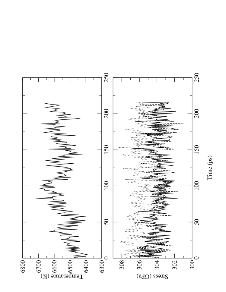
Figure 1: Time variation of temperature (upper panel) and the three components of stress tensor $P_{xx}$ (solid curve), $P_{yy}$ (dashed curve) and $P_{zz}$ (dotted curve) (upper panel), during a simulation of solid and liquid Fe coexisting at a pressure of 305 GPa. Simulations were performed on a system of 8000 atoms using the embedded-atom potential of Belonoshko et al. [8], with $c/a$ ratio of the h.c.p. solid equal to 1.64.

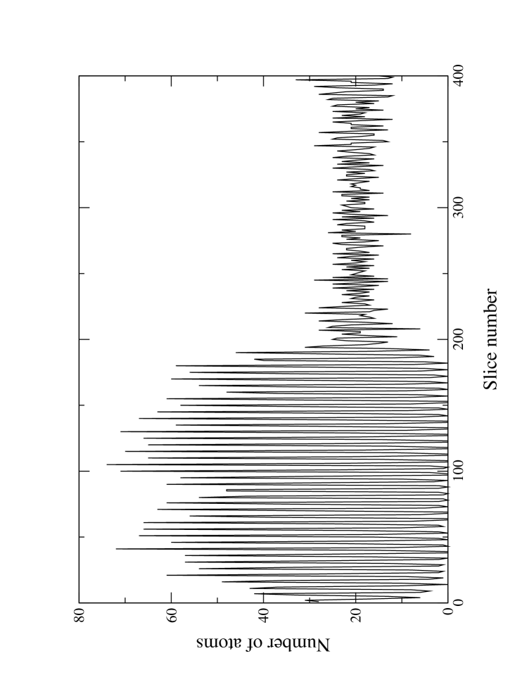
Figure 2: Density profile in a simulation of solid and liquid Fe coexisting at a pressure of 305 GPa. The system is divided into slices of equal thickness (0.35 Å) parallel to the solid-liquid interface, and graph shows number of atoms in each slice. Simulations were performed on a system of 8000 atoms using the embedded-atom potential of Belonoshko et al. [8].

In Fig. 1, we show the temperature of the system as a function of simulation time for $c/a=1.64$. We also show the three diagonal components of the stress tensor; the off-diagonal components fluctuate around their average value of zero, so there is no shear stress on the cell. After an initial equilibration period, one sees that the temperature and the pressure settle around the values $T=6550\pm 100$ K and $p=305\pm 1$ GPa. In Fig. 2, we display the density profile, calculated by dividing the simulation cell into 400 slices parallel to the liquid-solid interface and counting the number of atoms present in each slice. The profile shown corresponds to the last configuration in the simulation with $c/a=1.64$; a similar profile is observed in the simulation with $c/a=1.66$. It is easy to identify the solid and the liquid regions in the system: in the solid region the density is a periodic function of slice number, but in the liquid it fluctuates randomly around its average value. This confirms that we do indeed have coexisting solid and liquid in the cell. At 305 GPa, the melting temperature reported by Belonoshko with precisely the same EAM is 6680 K, which agrees with our value within the combined statistical errors.

We now correct the EAM reference melting temperature to obtain the fully ab initio melting temperature using the techniques presented in Sec. 2.4. In order to assess possible system-size errors, the free-energy corrections of Eqs. (8,9) were calculated with systems of 64, 150 and 288 atoms. To do this, we used the EAM reference model to generate long simulations for the solid and liquid separately. From these simulations we extract typically 50 and 100 statistically independent configurations for solid and liquid respectively, for which we calculate the DFT total energies $U_{\rm AI}$. The differences $\Delta U\equiv U_{\rm AI}-U_{\rm ref}$ are then used to compute the free-energy corrections and hence the shift of melting temperature (see Eq. (7)). The temperature was set equal to the value of 6550 K that emerges from the coexistence simulations, and volumes per atom of $v_{s}=7.05$ and $v_{l}=7.218$ Å³/atom were also deduced from the coexistence simulations; the pressure in both cases was 303 GPa. (The very small difference from the pressure of 305 GPa mentioned above is of no consequence.) From these two volumes we can extract the volume change on melting, which is $\Delta V\sim 2.5\%$, the same value reported as by Belonoshko et al. [8]. (The value from our ab initio free-energy work was 1.8 % at 305 GPa [5].) We also calculated the entropy of melting from the relation $TS_{\rm ref}^{ls}=E_{\rm ref}^{ls}+pV_{\rm ref}^{ls}$; the energy change on melting $E_{\rm ref}^{ls}$ was calculated using the two separate simulations of solid and liquid at $p=303$ GPa and $T=6550$K, and we obtained $S_{\rm ref}^{ls}=0.88$ k_B/atom; a similar value of $S^{ls}$ can be deduced from the work of Belonoshko et al. [8] by using their value for $V^{ls}$ and the Clausius-Clapeyron relation on the reported melting curve. (The value from our ab initio free-energy work was 1.07 $k_{\rm B}$/atom at 305 GPa [5].) The DFT energies were carefully checked for electronic $k$-point errors, as in our free-energy work [5, 17]. As expected from that work, $\Gamma$-point sampling for the 64-atom system underestimates the fully converged energies of liquid and solid by ca. 10 and 50 meV/atom respectively. With 150 atoms, $\Gamma$-point sampling gives negligible errors for the liquid, but an error of ca. $-8$ meV/atom for the solid. With 288 atoms, we have used only $\Gamma$-point sampling, but the indications are that $k$-point errors should be negligible for both phases.

We report in Table 1 the results for $\langle\Delta U\rangle_{\rm ref}$ and $\langle(\delta\Delta U)^{2}\rangle_{\rm ref}$ for the three system sizes, the results being already corrected for electronic $k$-point errors. An important feature of these results is that there is no discernible system size effect on these corrections within the statistical errors of 5 meV or less, so that systems of 64 atoms are adequate for calculating the corrections. From Eq. (7), this imples that the shift of $T_{\rm m}$ due to size errors will not more than $\sim 50$ K. In order to obtain the corrections $\Delta G$ to the Gibbs free energy, we need to include the term in $\Delta p^{2}$ in Eq. (9). We find that the pressure differences between the EAM and ab-initio systems are only 22 and 12 GPa for solid and liquid respectively, which give this term values of ca. 5 meV. From Table 1, we see that the free-energy differences between the ab initio and EAM systems have the effect of stabilizing the liquid with respect to the solid by about 35 meV/atom compared with the EAM. In order to obtain the correction to the melting temperature from Eq. (7), we use the value for the entropy of melting $S_{\rm ref}^{ls}$ of $0.88k_{\rm B}$/atom quoted above. This gives the first-order correction $T_{\rm m}^{\prime}=-450$ K, so that our corrected $T_{m}$ at 305 GPa is $6100\pm 100$ K. This result is in very close agreement with the free-energy approach, which at $p=305$ GPa gives $T_{m}=6100$ K. (This value is somewhat lower than the preliminary result of our free-energy calculations [4]; the downward revision came from a careful reanalysis of the anharmonic free energy of the h.c.p. crystal, as reported in Refs. [5, 17].)

Although the EAM of Belonoshko et al. [8] mimics our ab initio systems reasonably well, we have found that the model can be still further improved by refitting it to our ab initio energies of the solid and liquid. In doing this, we allowed only the repulsive potential and the strength of the embedding energy to change, so that only the parameters $n$, $\epsilon$ and $C$ are allowed to vary. These were adjusted to minimise the $\delta\Delta U$ fluctuations for the solid, while also maintaining the correct pressure. The new parameters are $n=5.93,\epsilon=0.1662$ eV, $C=16.55$, the parameters $a=3.4714$ Å and $m=4.788$ retaining their original values. We then repeated the coexistence simulation using this new EAM and obtained a coexistence temperature of $T_{m}=6200\pm 100$ K at a pressure of $p=323.5\pm 1$ GPa. The very small free-energy corrections (Table 2) slightly stabilize the solid, resulting in an increase of melting temperature of ca. 50 K to give $6250\pm 100$ K. The differences with the ab-initio pressures are negligible in this case, and the term in $\Delta p^{2}$ in Eq. (9) does not contribute to the free energy difference. At this pressure, the melting temperature from our free energy approach was $T_{m}=6290$ K [5], so that once again we find very good agreement between the two approaches.

4 Discussion and conclusions

We have advocated the aim of calculating the melting properties that follow from a chosen approximation for the exchange-correlation functional $E_{\rm xc}$, with the errors due to all other approximations being made negligible. We have stressed that in the free-energy approach the total energy of the reference model does not have to agree exactly with the ab initio total energy, since this approach includes the calculation of the free energy difference between the two systems. Up to now, no allowance has been made for such differences in the coexistence approach, but we have shown how corrections can be made so that the final results are again independent of the reference model. Our practical results for high-pressure Fe demonstrate that the two approaches then give the same melting temperatures, as would be expected.

Our analysis has implications for the way in which reference systems are constructed. In the free-energy approach, the crucial requirement of a reference model is that the fluctuations of the difference $\Delta U$ between the ab initio and reference energies be as small as possible; we have the freedom to use different reference models for the solid and liquid phases, and a constant offset between the ab initio and reference energies is of no consequence. In the coexistence approach, it seems clear that the model should be chosen so that the $\Delta G$ corrections, and the resulting shift of melting temperature away from that of the reference system, be as small as possible. This demands more of the reference system than in the free-energy approach. It is necessary but not sufficient that the $\Delta U$ fluctuations be small, in order that $\Delta G$ be small (see Eq. (9)). In addition, a constant energy offset will shift $T_{\rm m}$, if the offset is not identical in the two phases, since the same model must simultaneously reproduce the energetics of both. This implies that force matching [7, 19] may not always be a reliable way of constructing reference models: even if the reference and ab initio forces match precisely in both phases, there may still be a non-cancelling $\Delta U$ offset that will shift $T_{\rm m}$. In this sense, energy matching is safer than force matching.

Concerning finite-size errors, we have shown that these affect appreciably only the free-energy differences between the ab initio and reference systems, since in both approaches the calculations on the reference model will always be done on systems large enough to make size errors negligible. If anything, these errors may be more troublesome in the coexistence approach, because of the need to make the reference model fit both phases at once, so that the free-energy corrections may sometimes be larger. However, in our coexistence calculations on high-pressure Fe, we have shown that these errors are unlikely to shift $T_{\rm m}$ by more than $\sim$ 50 K.

In commenting on the strengths and weaknesses of the two approaches, we note that they differ mainly in the way of treating the thermodynamic properties of the reference model. In both approaches, corrections are then needed to obtain the properties of the ab initio system, and these involve ab initio simulations to perform thermodynamic integration or to compute the free-energy differences of Eq. (8). The melting properties of the reference model are probably more straightforward to calculate by the coexistence approach, since the free-energy approach requires rather intricate thermodynamic integrations. However, the heaviest computational effort comes in the calculation of the free-energy corrections, and here we believe the free-energy approach may have the advantage, since the effort can be reduced by using different reference systems for the two phases. In practice, we have found it very helpful to use both approaches, as in the work on Fe reported here.

	$\langle\Delta U\rangle_{\rm ref}/N$		$\langle(\delta\Delta U)^{2}\rangle_{\rm ref}/N$
$N$	Liquid	Solid	Liquid	Solid
64	$-6.940\pm 0.003$	$-6.909\pm 0.002$	$0.023\pm 0.004$	$0.014\pm 0.003$
150	$-6.934\pm 0.001$	$-6.912\pm 0.001$	$0.023\pm 0.003$	$0.009\pm 0.002$
288	$-6.939\pm 0.001$	$-6.909\pm 0.001$	$0.024\pm 0.004$	$0.014\pm 0.003$

Table 1: Thermal average $\langle\Delta U\rangle_{\rm ref}$ of the difference $\Delta U\equiv U_{\rm AI}-U_{\rm ref}$ of ab initio and reference energies, and thermal average $\langle(\delta\Delta U)^{2}\rangle_{\rm ref}$ of the squared fluctuations of $\delta\Delta U\equiv\Delta U-\langle\Delta U\rangle_{\rm ref}$, with averages evaluated in the ensemble of the reference system and normalized by dividing by the number of atoms $N$ (eV units). Results from simulations with difference $N$ are reported for liquid and solid Fe for the thermodynamic state $p=303$ GPa, $T=6550$ K. Reference model is the embedded-atom model of Belonoshko et al. [8].

	$\langle\Delta U\rangle_{\rm ref}/N$		$\langle(\delta\Delta U)^{2}\rangle_{\rm ref}/N$
$N$	Liquid	Solid	Liquid	Solid
64	$7.213\pm 0.002$	$7.200\pm 0.002$	$0.018\pm 0.003$	$0.009\pm 0.002$

Table 2: Thermal averages $\langle\Delta U\rangle_{\rm ref}$ and $\langle(\delta\Delta U)^{2}\rangle_{\rm ref}$ (eV units, see caption of Table 1) for the EAM reference model obtained by refitting that of Belonoshko et al. [8].

References

- [1] B. J. Alder and T. E. Wainwright, J. Chem. Phys. 27, 1208 (1957).
- [2] O. Sugino and R. Car, Phys. Rev. Lett. 74, 1823 (1995).
- [3] G. A. de Wijs, G. Kresse, and M. J. Gillan, Phys. Rev. B 57, 8223 (1998).
- [4] D. Alfè, M. J. Gillan, and G. D. Price, Nature, 401, 462 (1999).
- [5] D. Alfè, M. J. Gillan, and G. D. Price, Phys. Rev. B, submitted.
- [6] L. Vočadlo and D. Alfè, Phys. Rev. B, submitted.
- [7] A. Laio, S. Bernard, G. L. Chiarotti, S. Scandolo, and E. Tosatti, Science 287, 1027 (2000).
- [8] A. B. Belonoshko, R. Ahuja, and B. Johansson, Phys. Rev. Lett. 84, 3638 (2000).
- [9] J. R. Morris, C. Z. Wang, K. M. Ho, and C. T. Chan, Phys. Rev. B 49, 3109 (1994).
- [10] J. Q. Broughton and X. P. Li, Phys. Rev. B 35, 9120 (1987).
- [11] S. M. Foiles and J. B Adams, Phys. Rev. B 40, 5909 (1989).
- [12] J. Mei and J. W. Davenport, Phys. Rev. B 46, 21 (1992).
- [13] R. Agrawal and D. A. Kofke, Phys. Rev. Lett. 74, 122 (1995).
- [14] J. B. Sturgeon and B. B. Laird, Phys. Rev. B 62, 14720 (2000).
- [15] P. Hohenberg and W. Kohn, Phys. Rev. 136, B864 (1964); W. Kohn and L. Sham, Phys. Rev. 140, A1133 (1965); R. O. Jones and O. Gunnarsson, Rev. Mod. Phys. 61, 689 (1989); M. C. Payne, M. P. Teter, D. C. Allan, T. A. Arias, and J. D. Joannopoulos, Rev. Mod. Phys. 64, 1045 (1992); M. J. Gillan, Contemp. Phys. 38, 115 (1997); R. G. Parr and W. Yang, Density-Functional Theory of Atoms and Molecules, (Oxford University Press, Oxford, 1989).
- [16] A. B. Belonoshko, R. Ahuja, O. Eriksson, and B. Johansson, Phys. Rev. B 61, 3838 (2000).
- [17] D. Alfè, G. D. Price, and M. J. Gillan, Phys. Rev. B 64, 045123 (2001).
- [18] D. Frenkel and B. Smit, Understanding Molecular Simulation, Ch. 4 (Academic, New York, 1996).
- [19] F. Ercolessi and J. B. Adams, Europhys. Lett. 26, 583 (1994).
- [20] M. S. Daw, S. M. Foiles, and M. I. Baskes, Mat. Sci. Rep. 9, 251 (1993).
- [21] J.-P. Poirier, Introduction to the Physics of the Earth’s Interior (Cambridge University Press, Cambridge, England, 1991).
- [22] L. Vočadlo, D. Alfè, J. Brodholt, M. J. Gillan, and G. D. Price, Geophys. Res. Lett., 26, 1231 (1999).
- [23] L. Vočadlo, D. Alfè, J. P. Brodholt, G. D. Price, and M. J. Gillan, Phys. Earth Planet. Inter. 117, 123 (2000).
- [24] Y. Wang and J. Perdew, Phys. Rev. B 44, 13298 (1991).
- [25] J. P. Perdew, J. A. Chevary, S. H. Vosko, K. A. Jackson, M. R. Pederson, D. J. Singh, and C. Fiolhais, Phys. Rev. B 46, 6671 (1992).
- [26] P. E. Blöchl, Phys. Rev. B 50, 17953 (1994).
- [27] G. Kresse and D. Joubert, Phys. Rev. B 59, 1758 (1999).
- [28] D. Alfè, G. Kresse, and M. J. Gillan, Phys. Rev. B, 61, 132 (2000).
- [29] S. H. Wei and H. Krakauer, Phys. Rev. Lett., 55, 1200 (1985).
- [30] D. Vanderbilt, Phys. Rev. B 41, 7892 (1990).
- [31] G. Kresse and J. Furthmüller, Phys. Rev. B 54, 11169 (1996).
- [32] G. Kresse and J. Furthmüller, Comput. Mater. Sci. 6, 15 (1996).