Direct Measurement of the Spin Hamiltonian and Observation of
Condensation of Magnons in the 2D Frustrated Quantum Magnet Cs₂CuCl₄

Abstract

We propose a method for measuring spin Hamiltonians and apply it to the spin-1/2 Heisenberg antiferromagnet Cs₂CuCl₄, which shows a 2D fractionalized RVB state at low fields. By applying strong fields we fully align the spin moment of Cs₂CuCl₄ transforming it into an effective ferromagnet. In this phase the excitations are conventional magnons and their dispersion relation measured using neutron scattering give the exchange couplings directly, which are found to form an anisotropic triangular lattice with small Dzyaloshinskii-Moriya terms. Using the field to control the excitations we observe Bose condensation of magnons into an ordered ground state.

Understanding strongly correlated physics poses formidable mathematical difficulties and in only a few exceptional cases has the full many-body quantum problem been solved. Although theory takes the Hamiltonian ($\mathcal{H}$) as its starting point linking experimental data to this is often not possible. A method for measuring $\mathcal{H}$ directly would bridge this gap to theoretical approaches and in addition reveal the essential ingredients from which exotic quantum states emerge. Motivated by this we combine neutron scattering with high magnetic fields and make just such a determination of $\mathcal{H}$ taking the remarkable quantum magnet Cs₂CuCl₄ as a subject. We base our approach on overcoming spin couplings using large fields thus transforming the system into an effective ferromagnet, an easily solvable state. In addition we explore how the ordered ground state evolves with lowering field and interpret the results in the framework of Bose-Einstein condensation (BEC) of magnons.

The insulating magnet Cs₂CuCl₄ is an ideal subject for two reasons: First, its relatively weak ($\sim 4$ K) couplings can be overcome by current fields (at 8.44 T), and second, it shows highly unusual strongly correlated properties Coldea01 . Among the most fascinating are a low-field dynamics dominated by 2D highly dispersive continua characteristic of fractionalization of spinwaves into spin-1/2 spinons, exceptionally strong quantum renormalizations, and an unexplained $T=0$ disordered phase induced by weak fields along $b$ and $c$. Although Anderson first proposed a 2D fractionalized state in 1973 (the resonating valence bond state), the essential conditions for its existance have remained highly contentious Anderson73 . In light of this establishing what the special ingredients are in the Hamiltonian of Cs₂CuCl₄ is therefore very important.

The origins of strongly correlated phases lie in the uncertainty principle. For quantum magnets uncertainty is embedded in the noncommutation of the spin vector components ${\bm{S}}=\{S^{x},S^{y},S^{z}\}$ and the “true” direction of ${\bm{S}}$ cannot be known. For spins ${\bm{S}_{R}}$ on a lattice ${\bm{R}}$ coupled by the Heisenberg exchange Hamiltonian

$$\mathcal{H}=\frac{1}{2}\sum_{{\bm{R}},{\bm{\delta}}}J_{\bm{\delta}}{\bm{S}}_{\bm{R}}\cdot{\bm{S}}_{\bm{R}+\bm{\delta}}-g\mu_{B}BS_{\bm{R}}^{z}$$ (1)

the energy depends simultaneously on all three noncommuting components of each ${\bm{S}_{R}}$ (${\bm{\delta}}$ is a vector between sites and the last term an attendant magnetic field). Quantum uncertainty appears as a kinetic term ($S_{\bm{R}}^{+}S_{\bm{R}+\bm{\delta}}^{-}+S_{\bm{R}}^{-}S_{\bm{R}+\bm{\delta}}^{+}$) in the action on the spins which is most extreme for spin-1/2 where it flips pairs of spins e.g. $\uparrow\downarrow$ to $\downarrow\uparrow$, and the magnet fluctuates between many spin configurations. Semiclassically this kinetic action correlates particle motions (and creation) with others and can be so strong that new phases emerge as in Cs₂CuCl₄.

When large enough, the field $B$ in (1) prevails over the exchanges and the unique situation arises where the ground state of $\mathcal{H}$ is known and the one-particle excited states are exactly solved. The ground state consists of all spins up, which we denote $\Psi_{0}=|0\rangle,\;E_{0}=-Ng\mu_{B}BS+N/2\sum_{\bm{\delta}}J_{\bm{\delta}}S^{2}$, which is indeed that of a ferromagnet. There are $N$ orthonormal states with a single spin flip $\psi_{\bm{R}}=S_{{\bm{R}}}^{-}/\sqrt{2S}|0\rangle$ corresponding to all sites ${\bm{R}}$. When $\mathcal{H}$ acts on $\psi_{\bm{R}}$, it generates only other such one-spin-flip states because the total spin $S_{T}^{z}=\sum_{{\bm{R}}}S_{{\bm{R}}}^{z}$ is a constant-of-the-motion for $\mathcal{H}$. Because the Hamiltonian is invariant upon translation plane-wave states are diagonal: $\psi_{\bm{k}}\equiv N^{-1/2}\sum_{\bm{R}}\exp(-i{\bm{k}}\cdot{\bm{R}})\psi_{\bm{R}}$ where $\mathcal{H}\psi_{\bm{k}}=E({\bm{k}})\psi_{\bm{k}}$. The kinetic term causes hopping of these spin-flips through the lattice and the energy eigenvalues (for spins $S$=1/2) are

$$E({\bm{k}})=E_{0}+g\mu_{B}B-J_{\bm{0}}+J_{\bm{k}},\;J_{\bm{k}}={\frac{1}{2}}\sum_{\bm{\delta}}J_{\bm{\delta}}e^{i{\bm{k}}\cdot{\bm{\delta}}}$$ (2)

so that the one-spin-flip excitations disperse relative to the ground state with the relation, $\hbar\omega_{\bm{k}}=E({\bm{k}})-E_{0}=g\mu_{B}B-J_{\bm{0}}+J_{\bm{k}}$, which is a constant term plus $J_{\bm{k}}$, the Fourier transformed exchange couplings. These excitations are the familiar quantized harmonic spin-wave modes, magnons, which carry $\Delta S^{z}=-1$ and have Bose statistics. Since neutrons are spin-1/2 particles they scatter only by changing the total spin by $\Delta S=0,\pm 1$. For a system prepared in the fully-aligned state $|0\rangle$ neutrons can scatter inelastically only by exciting a single magnon through the matrix element $|\langle\psi_{\bm{k}}|S_{\bm{k}}^{-}|0\rangle|^{2}$ where $S_{\bm{k}}^{-}=N^{-1/2}\sum_{\bm{R}}\exp(-i{\bm{k}}\cdot{\bm{R}})S_{\bm{R}}^{-}$. $J_{\bm{k}}$ and so $J_{\bm{\delta}}$ of Eq. (1) can then be found from the measured dispersion $\hbar\omega_{\bm{k}}$.

The crystal structure of Cs₂CuCl₄ is orthorhombic (Pnma) with lattice parameters at 0.3 K of $a$=9.65 Å, $b$=7.48 Å, and $c$=12.35 Å. The magnetic $S=1/2$ Cu²⁺ ions are situated within distorted CuCl${}_{4}^{2-}$ tetrahedra. Layers ($bc$ plane) of these tetrahedra are separated by Cs⁺ ions and are stacked with an offset giving the structure illustrated in Fig. 1(a). The strongly correlated physics derives from the “isosceles” triangular lattice arrangement of spins in the layers with antiferromagnetic exchange paths $J\equiv J_{[0,1,0]}$ and $J^{\prime}\equiv J_{[0,1/2,\pm 1/2]}$. The triangular geometry allows a large configuration space for fluctuations and is presumably crucial to fractionalization.

To measure $\hbar\omega_{\bm{k}}$ the V2 cold-neutron triple-axis spectrometer at the BER-II reactor at HMI in Berlin was used. A large (3.6 g) high-quality single crystal of Cs₂CuCl₄ was mounted in the (0,$k$,$l$) scattering plane on a dilution refrigerator insert with base temperature of 50 mK. The VM-1 cryomagnet provided fields up to 14.5 T along $a$. The spectrometer was configured with a vertically-focused monochromator (PG002) and a horizontally focused PG002 analyzer to select scattered neutrons with fixed $k_{f}=1.2$ or 1.35 Å^-1.

A magnetic field of 12 T, much larger than the saturation field (8.44 T), was used to open a significant energy gap of 0.435(8) meV to the first excited states. Temperatures below 200 mK ensured that the thermally introduced population of spin flips was less than 1 per $10^{11}$ spins. No magnetostructural distortions were observed and the origin of superexchange in high-energy electronic bonds means that the coupling constants are unperturbed by the field. Only one magnon scattering events were observed and their energy and wavevector dependence mapped out. Fig. 2(c) shows a typical scan. Two resolution limited peaks are seen separated by a small energy of 0.084(2) meV; this splitting is due to an additional anisotropy as explained below.

The measured one-magnon dispersion relations are graphed in Fig. 2(a). The considerable dispersion along both [0$k$0] and [00$l$] in the $bc$ plane indicates strong 2D character. The overall dispersion follows $\hbar\omega_{\bm{k}}$ with $J_{\bm{k}}=J\cos(2\pi k)+2J^{\prime}\cos(\pi k)\cos(\pi l)$ where $J=0.374(5)$ meV and $J^{\prime}=0.128(5)$ meV, the couplings in Fig. 1(a) (${\bm{k}}=(h,k,l)$ is expressed in units of ($2\pi/a,2\pi/b,2\pi/c)$). The small splitting into two magnon branches is characterized well by modified dispersions $\hbar\omega_{\bm{k}}^{\pm}=g\mu_{B}B-J_{\bm{0}}+J_{\bm{k}}\pm D_{\bm{k}},D_{\bm{k}}=2D_{a}\sin(\pi k)\cos(\pi l)$ with $D_{a}=0.020(2)$ meV. This is surprising because whereas $J_{\bm{k}}$ is a sum of cosine terms, $D_{\bm{k}}$ is sinusoidal. The physical meaning of this is that a left moving magnon (of a certain type) has different energy from a right moving one $\hbar\omega_{k}^{\pm}\neq\hbar\omega_{-k}^{\pm}$; the two magnon branches actually cross over at $k=0$, $\hbar\omega_{k}^{\pm}=\hbar\omega_{-k}^{\mp}$, and such a situation can come about only if an exchange with a sense of direction is present.

Dzyaloshinskii and Moriya (DM) Moriya60 proposed just such an exchange interaction many years ago. They showed that spin-orbit couplings in the superexchange can generate a coupling of the form ${{\bm{D}}_{ij}}\cdot({\bm{S}}_{i}\times{\bm{S}}_{j})$. Their interaction is of higher-order and therefore much weaker than Heisenberg exchange and can occur only when the superexchange pathways do not have centers of inversion which is indeed the case in Cs₂CuCl₄.

In the ordered structure (below $T_{N}$=620 mK and $B=0$) the moments lie almost within the $bc$ plane which would happen if the most important ${\bm{D}}_{ij}$ vector in Cs₂CuCl₄ was directed along the $a$-axis, and the observed wavevector dependence, $\sin(\pi k)\cos(\pi l)$, of $D_{\bm{k}}$ suggests that the important DM interaction is along the same zig-zag bonds as $J^{\prime}$ in the 2D planes. Considering these bonds only, and making the approximation that ${\bm{D}}^{\pm}=(\pm D_{a},0,0)\equiv{\bm{D}}_{a}^{\pm}$ we obtain using symmetry

$$\mathcal{H}_{DM}^{\pm}\!\!=\!\frac{1}{2}\!\sum_{\bm{R}}{\bm{D}}_{a}^{\pm}\cdot{\bm{S}_{\bm{R}}}\times[-{\bm{S}_{\bm{R}+\bm{\delta}_{1}}}-{\bm{S}_{\bm{R}+\bm{\delta}_{2}}}+{\bm{S}_{\bm{R}+\bm{\delta}_{3}}}+{\bm{S}_{\bm{R}+\bm{\delta}_{4}}}]$$ (3)

where the labels $\bm{\delta}_{1-4}$ refer to Fig. 1(a) and the $\pm$ has been introduced because there are two distinct layers shown in Fig. 1(b) which are inverted versions of each other with DM vectors pointing in opposite directions. Like the Heisenberg coupling this DM interaction also conserves $S_{T}^{z}$ and plane-wave solutions remain diagonal; $\mathcal{H}_{DM}^{\pm}\psi_{\bm{k}}=\pm D_{\bm{k}}\psi_{\bm{k}}$ where $D_{\bm{k}}=2D_{a}\sin(\pi k)\cos(\pi l)$ as observed. The DM interaction then explains the observed sinusoidal components of $\hbar\omega_{\bm{k}}^{\pm}$ and the fact that there are two modes - one for each type of layer.

Table 1: Hamiltonian parameters ($B>B_{C}$)(see text) versus the quantum renormalized ($B=0$) parameters from Coldea01 .

Parameter	$B>B_{C}$	$B=0$	Renormalization
$J$ (meV)	0.374(5)	0.62(1)	1.65(5)
$J^{\prime}$ (meV)	0.128(5)	0.117(9)	0.91(9)
$J^{\prime\prime}$ (meV)	0.017(2)	-	-
$D_{a}$ (meV)	0.020(2)	-	-
$\epsilon$ (rlu)	0.053(1)	0.030(2)	0.56(2)

The fact that Cs₂CuCl₄ orders three dimensionally means that there must be an interaction $J^{\prime\prime}_{\bm{k}}$ between layers. We introduce operators $a_{\bm{k}}^{\dagger}$ and $b_{\bm{k}}^{\dagger}$ that create the two types of magnons on the different layers. The full Hamiltonian with DM and interlayer couplings is:

$$\mathcal{H}\!=\!\!\sum_{\bm{k}}\!\left[\!\begin{array}[]{cc}a_{\bm{k}}^{{\dagger}}&b_{\bm{k}}^{{\dagger}}\end{array}\!\right]\!\!\left[\begin{array}[]{cc}{\hbar\Omega_{\bm{k}}-J^{\prime\prime}_{\bm{0}}}+D_{\bm{k}}&J^{\prime\prime}_{-\bm{k}}\\ J^{\prime\prime}_{\bm{k}}&{\hbar\Omega_{\bm{k}}-J^{\prime\prime}_{\bm{0}}}-D_{\bm{k}}\end{array}\!\right]\!\!\left[\!\begin{array}[]{c}a_{\bm{k}}\\ b_{\bm{k}}\end{array}\!\right]$$

where $\hbar\Omega_{\bm{k}}=g\mu_{B}B-J_{\bm{0}}+J_{\bm{k}}$ is the magnon dispersion for $D_{\bm{k}}=J^{\prime\prime}_{\bm{k}}=0$. Diagonalizing this Hamiltonian gives the new dispersion relations

$$\hbar\omega_{\bm{k}}^{\pm}=\hbar\Omega_{\bm{k}}-J^{\prime\prime}_{\bm{0}}\pm\sqrt{D_{\bm{k}}^{2}+|J^{\prime\prime}_{\bm{k}}|^{2}},$$ (4)

and for the case of interlayer nearest neighbor coupling [see Fig. 1(b)] ($J^{\prime\prime}_{\bm{k}}$=$J^{\prime\prime}\cos(\pi h)e^{-i2\pi l\zeta}$) the relative intensity of the two modes is

$$\frac{I^{+}_{\bm{k}}}{I^{-}_{\bm{k}}}=\frac{1+\cos(2\pi l\zeta)\sin(2\theta_{\bm{k}})}{1-\cos(2\pi l\zeta)\sin(2\theta_{\bm{k}})},$$ (5)

with $\theta_{\bm{k}}=\tan^{-1}[J^{\prime\prime}\cos(\pi h)/(\sqrt{D_{\bm{k}}^{2}+|J^{\prime\prime}_{\bm{k}}|^{2}}+D_{\bm{k}})]$ and where the total inelastic intensity $I^{+}_{\bm{k}}+I^{-}_{\bm{k}}$ is independent of wavevector. Here $\zeta$=0.34 is the relative offset along $c$ between adjacent layers. Fitting the above model (Eqs.(4) and (5)) to the data yields the excellent fits shown in Figs. 2(a)-(d) with the fitted parameters listed in the first column of Table I and $g_{a}$=2.19(1). The total inelastic intensity shown in Fig. 2(b) is nearly independent of ${\bm{k}}$ as predicted. The relative intensity of the two modes (where they could be resolved) is shown in Fig. 2(d). We conclude that all other couplings in Cs₂CuCl₄ are much smaller. Dipolar energies and g-tensor anisotropies are small and neglected here.

Upon decreasing field the magnon energies reduce by the additive Zeeman term $g\mu_{B}B$ [see Fig. 3(a)]. At the critical field $B_{C}$=8.44(1) T the gap closes at the dispersion minima $\bm{\tau}\pm\bm{Q}$, $\bm{Q}$=(0.5+$\epsilon$)$\bm{b}^{\ast}$, $\epsilon$=0.053(1). At those wavevectors Bragg peaks appear below $B_{C}$ indicating transverse (off-diagonal) long-range order. This order is an example of BEC in a dilute gas of magnons induced by changing the “chemical potential” $|B_{C}-B|$ Matsubara56 . The measured spin order forms an elliptical cone around the field direction $\langle\bm{S}_{\bm{R}}\rangle\!=\!\pm\hat{\bm{b}}S_{b}\cos\bm{Q}\!\cdot\!\bm{R}+\hat{\bm{c}}S_{c}\sin\bm{Q}\!\cdot\!\bm{R}+\hat{\bm{a}}S_{a}$ (odd/even $\pm$ layers contrarotate) where $S_{b}>S_{c}$ as illustrated in Fig. 3(e). In fact this order corresponds exactly to the simultaneous condensation of contrarotating magnons $\omega_{-\bm{Q}}^{-}$ and $\omega_{+\bm{Q}}^{-}$ [see Fig. 3(d)] with gap closure at $B_{C}$; a mean-field calculation Nikuni95 ; wavefunctions of this state gives an elliptical cone with asymmetry $(\cos\theta_{\bm{Q}}+\sin\theta_{\bm{Q}})/(\cos\theta_{\bm{Q}}-\sin\theta_{\bm{Q}})$=1.52(6) in agreement with the observed ratio $S_{b}/S_{c}$=1.55(10) just below $B_{C}$. The asymmetry is a combined effect of interlayer coupling $J^{\prime\prime}$ and alternation of $\bm{D}^{\pm}$ between layers and rapidly decreases as the field is lowered due to increased inter-particle interactions and fluctuations, $S_{b}/S_{c}$=1.1(1) below 7 T.

The effect of fluctuations and interactions on the order as field decreases is quantified in Fig. 3(b-c): Fig. 3(b) shows the off-diagonal order parameter $S_{c}$. Close to $B_{C}$ it is described by a power law (solid line) $S_{c}$$\sim$$|B_{C}-B|^{\beta}$ with $\beta$=0.33(3), significantly below the value $\beta$=0.5 expected for mean-field (3D) BEC Matsubara56 . The magnetization $S_{a}$ obtained from susceptibility measurements longpaper is plotted in the inset of Fig. 3(c). It shows that the boson density is not linear versus $|B_{C}-B|$ but rather shows a deviation that may be logarithmic Sachdev94 ; and finally the wavevector of the condensate $Q=0.5+\epsilon(B)$ is plotted in Fig. 3(c). $Q$ varies strongly with field indicating that magnon-magnon interactions are important even at low density and renormalize the condensate wavevector. The above features deviate significantly from mean-field (3D) behavior Nikuni00 and could be associated with the 2D nature of the magnons. In two dimensions interactions can qualitatively change the scaling behavior such as by introducing non-linear, log corrections to the magnetization curve Sachdev94 .

In summary, we have determined the Hamiltonian of the quasi-2D quantum magnet Cs₂CuCl₄ using a new experimental method and show that it is a 2D anisotropic triangular system. We also measured transverse (off-diagonal) order with field below saturation, an example of Bose-Einstein condensation of magnons. Our methods are general and could be used to reveal exchanges and quantum renormalizations for systems as diverse as random magnets, quantum antiferromagnets and spin glasses.

We would like to thank P. Vorderwisch for technical support and R.A. Cowley, A.M. Tsvelik and F.H.L. Essler for stimulating discussions. ORNL is managed for the US DOE by UT-Battelle, LLC, under contract DE-AC05-00OR22725. Financial support was provided by the EU through the Human Potential Programme under IHP-ARI contract HPRI-CT-1999-00020.

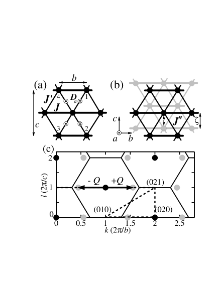
Figure 1: (a) Magnetic couplings in a 2D triangular layer in Cs₂CuCl₄: strong bonds $J$ (heavy lines $\parallel b$), smaller frustrating zig-zag bonds $J^{\prime}$ (thin lines). $D_{a}$ are the Dzyaloshinskii-Moriya (DM) couplings along the zig-zag bonds; the signs $\otimes,\odot$ refer to interactions originating at the central spin ${\bm{S}_{\bm{R}}}$, see Eq. (3). (b) Odd (black) and even (grey) layers are stacked successively along $a$ (inter-layer spacing $a/2$) with an offset $\zeta$=0.34 along $c$. $J^{\prime\prime}$ (dashed arrow) is the nearest-neighbor inter-layer exchange. (c) ($b^{*},c^{*}$) reciprocal plane showing the near-hexagonal Brillouin zones (thin lines) of the triangular lattice in (a). Black points are zone centers ($\bm{\tau}$) and grey points at $\bm{\tau}\pm\bm{Q}$ mark dispersion gap minima in the saturated phase ($B>B_{C}$) and where Bragg peaks appear below $B_{C}$.

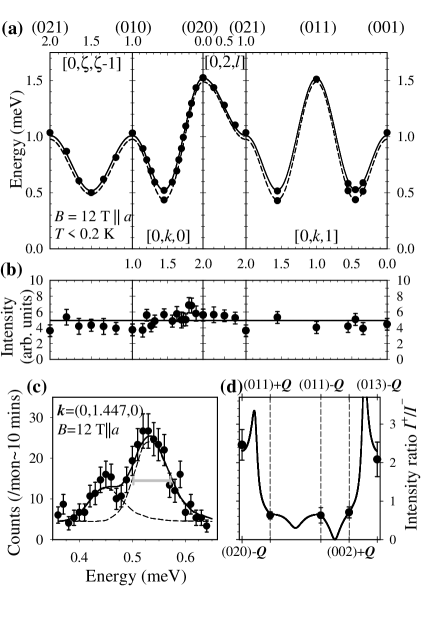
Figure 2: (a) Magnetic dispersion relations in the saturated phase ($B$=12 T$\parallel$$a$, $T<$0.2 K) along symmetry directions in the 2D plane (heavy dashed lines in Fig. 1(c)). Solid and dashed lines are fits to Eq. (4) with parameters in Table I. (b) Observed integrated inelastic intensity compared with predictions for the fully-polarized eigenstate (solid line). (c) Excitations lineshape observed along a constant-wavevector scan at the minimum gap $\bm{k}$=(0,1.447,0). Solid line is a fit to Eqs. (4-5) convolved with the instrumental resolution (horizontal grey bar indicates the full-width-half-maximum of the energy resolution).(d) Relative intensity of the two magnon modes compared with Eq. (5) (solid line).

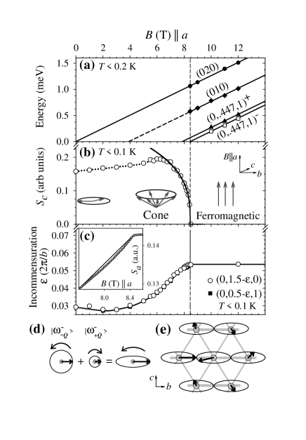
Figure 3: (a) Magnon energies vs. field in the saturated phase. Solid lines are fits to a linear behavior as expected for $\Delta S^{z}=-1$ eigenstates with $g$-factor $g_{a}$=2.18(1). (0,0.447,1)^± label the two magnon modes resolved at the minimum gap in scans such as in Fig. 2(c). (b) Amplitude of perpendicular ordered moment $S_{c}$ in the cone phase vs. field. Solid line is a power-law fit. (c) Incommensuration ($\epsilon$=$Q$-0.5) vs. field (solid line is guide to the eye). Inset: magnetization vs. field longpaper ($T$=30 mK) compared with a linear behavior (solid line). (d) Superposition of contrarotating magnons $\omega_{\pm\bm{Q}}^{-}$ wavefunctions of different amplitudes (large and small circle) gives the elliptical order in $bc$ plane shown schematically for odd layers in (e) (arrows are ordered spins). Even layers have opposite sense of rotation.

References

- (1) R. Coldea et al., Phys. Rev. Lett. 86, 1335 (2001).
- (2) P.W. Anderson, Mat. Res. Bull. 8, 153 (1973);V. Kalmeyer and R.B. Laughlin, Phys. Rev. Lett. 59, 2095 (1987); R. Moessner and S.L. Sondhi, Phys. Rev. Lett. 86, 1881 (2001); S. Sachdev, Phys. Rev. B 45, 12377 (1992); C.H. Chung et al J.Phys.: Condens. Matter 13, 5159 (2001).
- (3) I. Dzyaloshinskii, J. Phys. Chem. Solids 4, 241 (1958); T. Moriya, Phys. Rev. 120, 91 (1960).
- (4) T. Matsubara and H. Matsuda, Prog. Theor. Phys. 16, 569 (1956).
- (5) T. Nikuni, H. Shiba, J. Phys. Soc. Japan 64, 3471 (1995).
- (6) The two magnon wavefunctions are = + and =+, where are plane-wave superpositions of single spin flip states localized on the odd/even layers.
- (7) R. Coldea et al., (in preparation).
- (8) S. Sachdev et al., Phys. Rev. B 50, 258 (1994).
- (9) An example of 3D BEC of magnons was discussed in T. Nikuni et al, Phys. Rev. Lett. 84, 5868 (2000).