How to detect edge electron states in (TMTSF)₂X and $\bf Sr_{2}RuO_{4}$ experimentally

Abstract

We discuss a number of experiments that could detect the electron edge states in the organic quasi-one-dimensional conductors $\rm(TMTSF)_{2}X$ and the inorganic quasi-two-dimensional perovskites $\rm Sr_{2}RuO_{4}$. We consider the chiral edges states in the magnetic-field-induced spin-density-wave (FISDW) phase of $\rm(TMTSF)_{2}X$ and in the time-reversal-symmetry-breaking triplet superconducting phase of $\rm Sr_{2}RuO_{4}$, as well as the nonchiral midgap edge states in the triplet superconducting phase of $\rm(TMTSF)_{2}X$. The most realistic experiment appears to be an observation of spontaneous magnetic flux at the edges of $\rm Sr_{2}RuO_{4}$ by a scanning SQUID microscope.

1 Introduction

Edge electron states in various materials attracted a great deal of attention recently. In this paper, we discuss some experiments proposed to observe the effects of such states in the organic quasi-one-dimensional (Q1D) conductors $\rm(TMTSF)_{2}X$ and the inorganic quasi-two-dimensional perovskites $\rm Sr_{2}RuO_{4}$. For general overviews of these materials, see Refs. [1] and [2], respectively. The purpose of the paper is to encourage practical realization of these experiments by summarizing basic ideas and giving quantitative order-of-magnitude estimates without going into deep theoretical physics and mathematical formalism. The latter can be found in the cited references.

In general, a system with an energy gap has delocalized electron states in the bulk with energies above and below the energy gap. However, it may also have bound states with energies inside the gap, which are localized near the sample edges or other inhomogeneities. The energy gap may be of different origin, e.g. insulating or superconducting. In Sec. 2, we study the case where the gap is produced by the magnetic-field-induced spin-density wave (FISDW) in $\rm(TMTSF)_{2}X$. In Secs. 3 and 4, we consider triplet superconducting states in $\rm(TMTSF)_{2}X$ and $\rm Sr_{2}RuO_{4}$.

2 Chiral edge states in the FISDW phase of $\rm(TMTSF)_{2}X$

$\rm(TMTSF)_{2}X$ are Q1D crystals consisting of conducting chains parallel to the a axis, with substantial interchain coupling in the b direction and much weaker coupling in the c direction [1], along which we select the $x$, $y$, and $z$ axes. The lattice spacings are $a=0.73$ nm, $b=0.77$ nm, and $c=1.35$ nm, whereas the typical sample dimensions are $L_{x}=2$ mm and $L_{y}\approx L_{z}=0.2$ mm. Thus, a typical sample contains $\mathcal{N}_{c}=L_{y}L_{z}/bc\approx 4\times 10^{10}$ chains and $\mathcal{N}_{l}=L_{z}/c\approx 1.5\times 10^{5}$ layers. When a magnetic field $H$ is applied along the c axis, it causes a phase transition into the FISDW state, which exhibits the integer quantum Hall effect (IQHE). The Hall conductivity per one (a,b) layer is $\sigma_{xy}=2Ne^{2}/h$, where $N$ is a small, $H$-dependent integer number, $e$ is the electron charge, and $h$ is the Planck constant. In general, it is expected that $N$ chiral gapless edge states should exist in an IQHE system along the perimeter of the sample, as sketched in Fig. 1. Such edge states were indeed constructed theoretically for FISDW in Refs. [3, 4].

2.1 Time-of-flight experiment

As was shown in Refs. [3, 4], the edge states travel with the group velocities $v_{\perp}=Nb\Delta/\hbar\approx N\times 300$ m/s perpendicular to the chains and the Fermi velocity $v_{F}\approx 190$ km/s parallel to the chains, where $\Delta\approx 3$ K is the FISDW gap. In the time-of-flight experiment described in Ref. [4], a pulse, sent by the pulser, perturbs the edge states (see Fig. 1). This perturbation is carried downstream and reaches the detector D1 with the delay time $t=L_{y}/2v_{\perp}\approx 0.33$ $\mu$s and the detector D2 with the greater delay $3t$. The pulse can be electric (perturbing the occupation number of the edge states), or magnetic (creating spin polarization of the edge states), or thermal (perturbing the electron temperature of the edge states). The time-of-flight experiments with electric perturbations have been successfully performed in semiconducting QHE systems [5].

Figure 1: Sketch of the proposed time-of-flight experiment. The arrows indicate the directions of the edge states velocities $v_{\perp}$ and $v_{F}$. The thin lines indicate the conducting chains of $\rm(TMTSF)_{2}X$. The pulser sends a pulse, which is detected at different times by the detectors D1 and D2.

2.2 Specific heat

Since the chiral edge states are gapless, their the specific heat $C_{e}$ is linear in temperature $T$ and should dominate at low temperatures, where the bulk contribution is frozen out because of the FISDW gap $\Delta$. The edge specific heat per one chain is $C_{e}/T=2\pi k_{B}^{2}/3\Delta\approx 10^{-23}$ $\rm J/K^{2}$, where $k_{B}$ is the Boltzmann constant [4]. Multiplying this number by the total number of chains $\mathcal{N}_{c}\approx 4\times 10^{10}$, we obtain the total edge specific heat $4\times 10^{-13}$ $\rm J/K^{2}$. This value is smaller than the bulk specific heat in the normal state by the factor $2\xi/L_{x}\approx 0.5\times 10^{-3}$ (where $\xi=\hbar v_{F}/\Delta\approx 0.5$ $\mu$m is the coherence length), but it may be still measurable with a sensitive technique [6].

2.3 Thermal quantum Hall effect

1D chiral electron gas of temperature $T$ carries thermal current $\dot{Q}=\pi^{2}k_{B}^{2}T^{2}/6h$. Let us consider a FISDW sample with a heat source on the left, a heat drain on the right, and two thermometers $T_{1}$ and $T_{2}$ on the sides, as show in Fig. 2. The circulating edge current raises its temperature to $T_{1}$ by gaining thermal energy from the heat source and flows along the top edge of the bar maintaining that temperature (assuming no heat loss) until it reaches the heat drain. There the edge current loses its thermal energy, drops its temperature to $T_{2}$, and returns along the bottom edge maintaining that temperature. The net heat current from the source to the drain is

$$\dot{Q}_{x}=\dot{Q}_{1}-\dot{Q}_{2}=K_{xy}\,\delta_{y}T,\;\;\;\frac{K_{xy}}{T}=2N\frac{\pi^{2}k_{B}^{2}}{3h},$$ (1)

where $K_{xy}$ is the thermal Hall conductance, $\delta_{y}T=T_{1}-T_{2}$ is the temperature difference in the $y$ direction, and $T=(T_{1}+T_{2})/2$ is the average temperature of the edges. Eq. (1) demonstrates the thermal QHE proposed in Ref. [7]. Both the thermal and electrical Hall conductances are quantized with the same integer $N$ and are related to each other by the Wiedemann-Franz law for free electrons [7]. Detection of the thermal QHE will therefore confirm the existence of the chiral edge states in the FISDW phase. The quantum of thermal Hall conductance per one layer is $\pi^{2}k_{B}^{2}/3h=0.946\times 10^{-12}$ $\rm W/K^{2}$. The total thermal Hall conductance is obtained by multiplying this number by the number of layers $\mathcal{N}_{l}\approx 1.5\times 10^{5}$. The quantum of thermal conductance has been measured in the state-of-the-art experiments [8].

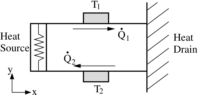
Figure 2: Sketch of the thermal quantum Hall effect experiment. The heat currents $\dot{Q}_{1}$ and $\dot{Q}_{2}$ are carried along the edges with the temperatures $T_{1}$ and $T_{2}$.

The above consideration assumed an idealized case where the longitudinal thermal conductances $K_{xx}$ and $K_{yy}$ are zero. In general, there will be nonzero temperature gradients in both $x$ and $y$ directions:

$$(\delta_{x}T,\delta_{y}T)={\dot{Q}_{x}\over K_{xx}K_{yy}+K_{xy}^{2}}(K_{yy},K_{xy}).$$ (2)

Because of the Wiedemann-Franz law, we expect that $K_{xx}K_{yy}\ll K_{xy}^{2}$ in the QHE regime, where $\sigma_{xx}\sigma_{yy}\ll\sigma_{xy}^{2}$. Then Eq. (1) approximately holds. However, there also exist phonon contributions to $K_{xx}$ and $K_{yy}$. In (TMTSF)₂ClO₄, the longitudinal thermal conductance per layer due to phonons is $K_{xx}/T\approx 5\times 10^{-11}\rm~{}W/K^{2}$ at $T\approx 0.2~{}\rm K$ and shows a power-law temperature dependence [9]. The phonon contribution is comparable to the quantum of $K_{xy}$ and can be made even smaller at lower temperatures, so an observation of the thermal QHE in the FISDW state of $\rm(TMTSF)_{2}X$ is feasible. In general, the thermal Hall conductance can be determined from the relation $K_{xy}=K_{yy}\,\delta_{y}T/\delta_{x}T$ [10].

3 Midgap Andreev edge states in the triplet superconducting phase of $\rm(TMTSF)_{2}X$

Figure 3: Conductances $G$ as functions of voltage $eV=E$ calculated for tunneling into the edges perpendicular (left panel) and parallel (right panel) to the chains in $\rm(TMTSF)_{2}X$. Here $T$ is not a temperature, but the transmission coefficient of tunneling barrier.

In $\rm(TMTSF)_{2}X$, the upper critical magnetic field $H_{c2}$ exceeds the Pauli paramagnetic limit by a factor greater than 4 [11], and the Knight shift does not change between the normal and superconducting states [12]. This indicates the triplet character of superconductivity in these materials [13, 14]. The triplet order parameter can be written as $\langle\psi_{\alpha}({\bf k})\psi_{\beta}(-{\bf k})\rangle\propto\epsilon_{\alpha\bar{\alpha}}[\mbox{\boldmath$\sigma$}_{\beta}^{\bar{\alpha}}\cdot\mbox{\boldmath$\Delta$}({\bf k})]$, where $\alpha$ and $\beta$ are the spin indices, $\sigma$ are the spin Pauli matrices, and $\epsilon_{\alpha\bar{\alpha}}=i\sigma^{y}_{\alpha\bar{\alpha}}$ is the antisymmetric spin metric tensor. We only consider the case of a uniform spin orientation: $\mbox{\boldmath$\Delta$}({\bf k})={\bf d}\,\Delta({\bf k})$, where d is a unit vector. The simplest triplet pairing potential $\Delta({\bf k})$ is an odd function of $k_{x}$, i.e. it has opposite signs on the two sheets of the Fermi surface located near $\pm k_{F}$. This sign change results in formation of Andreev bound states with energies exactly in the middle of the energy gap (midgap states) at the edges perpendicular to the chains, as explained in Ref. [15] (see also [16]). Unlike in the FISDW case discussed in Sec. 2, these midgap edge states are not chiral.

3.1 Tunneling experiment

Conceptually, the most straightforward way to detect the midgap edge states is by electron tunneling between a normal metal and the superconducting $\rm(TMTSF)_{2}X$. Tunneling into the edges perpendicular and parallel to the chains should exhibit a zero-bias peak and a gap, as shown in the left and right panels of Fig. 3, correspondingly. Unfortunately, it turned out difficult to achieve good tunneling junctions with the organic $\rm(TMTSF)_{2}X$. Below we discuss alternative experiments.

3.2 Paramagnetic spin response

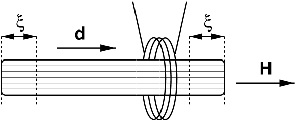
Figure 4: Schematic experimental setup to measure magnetic susceptibility of the edge states localized at the ends of the chains in superconducting $\rm(TMTSF)_{2}X$.

When a magnetic field $H$ is applied parallel to the vector d, the energies on the spin-up and spin-down midgap states split because of the Zeeman effect. At zero temperature, only the lower-energy states would be occupied, thus the edge states should be spin-polarized, yielding the magnetic moment $\mu_{B}/2=4.6\times 10^{-24}$ A m² per chain ($\mu_{B}$ is the Bohr magneton), or $\mathcal{N}_{c}\mu_{B}/2=1.8\times 10^{-13}$ A m² for the whole edge [15]. At a finite temperature, the edges would exhibit a Curie-like paramagnetic spin response to the magnetic field, opposite to the diamagnetic Meissner response of the bulk.

In order to perform the experiment proposed in Ref. [15], it is necessary to know the orientation of vector d. The theoretical analysis [14] of the $H_{c2}$ anisotropy [11] indicates that ${\bf d}\|{\bf a}$. However, recent Knight shift measurements [17] indicate that ${\bf d}\|{\bf c}$. We will consider the former case below. In the latter case, magnetic field ${\bf H}\|{\bf c}$ would quickly suppress superconductivity by the orbital effect. In the case ${\bf d}\|{\bf a}$, local magnetic susceptibility could be measures using a coil, as shown in Fig. 4, or by another method. As the coil approaches to the sample end, magnetic susceptibility should change sign from diamagnetic to paramagnetic because of the edge states contribution. They are localized within the coherence length $\xi=\hbar v_{F}/\Delta_{0}=0.6$ $\mu$m, where $\Delta_{0}\approx 0.22$ meV is the superconducting gap [1].

3.3 Schottky anomaly in specific heat

For ${\bf H}\|{\bf d}$, the Zeeman-split edge states effectively form a two-level system. It should exhibit the Schottky anomaly in specific heat:

$$C_{e}=\mathcal{N}_{c}k_{B}\left(\frac{\mu_{B}H/2k_{B}T}{\cosh(\mu_{B}H/2k_{B}T)}\right)^{2},$$ (3)

where $\mathcal{N}_{c}\approx 4\times 10^{10}$ is the total number of chains. Eq. (3) reaches the maximum $C_{\rm max}/\mathcal{N}_{c}=0.44~{}k_{B}=6.1\times 10^{-24}~{}\rm J/K$ at the temperature $T_{\rm max}=\mu_{B}H/2.4k_{B}$ proportional to the magnetic field. In order to avoid the contribution from the extended bulk states above the gap, the temperature should be lower than the energy gap: $T\ll\Delta_{0}$, thus the magnetic field should be well below the Pauli limiting field: $\mu_{B}H\ll\Delta_{0}$.

4 Chiral Andreev edge states in the superconducting $\rm Sr_{2}RuO_{4}$

$\rm Sr_{2}RuO_{4}$ is a quasi-two-dimensional perovskite with the superconducting transition temperature $T_{c}=1.5$ K. The main Fermi surface is a cylinder of radius $k_{F}=7.5\times 10^{9}~{}\rm m^{-1}$, and the interlayer spacing is $c=1.3$ nm [18]. We assume the typical sample dimensions to be $L_{x}=L_{y}=2$ mm and $L_{z}=1.3$ mm, which makes $\mathcal{N}_{l}=L_{z}/c=10^{6}$ layers.

The superconducting pairing in $\rm Sr_{2}RuO_{4}$ is believed to be triplet and chiral. The simplest proposed pairing potential has the form $\Delta({\bf k})=\Delta_{0}(k_{x}\pm ik_{y})/k_{F}$ [19]. More recently, it was suggested that the gap $\Delta_{0}$ is a real function of k with the nodes. The theoretical fit [20] of the tunneling data supports the horizontal lines of nodes, with $\Delta_{0}$ being a periodic function of $k_{z}$. However, in the present paper, we only consider the simplest case $\Delta_{0}=\rm const$ without nodes, because we focus on the question whether the superconductivity in $\rm Sr_{2}RuO_{4}$ is chiral. The main experimental evidence for that is the change of muon spin relaxation time at $T_{c}$ [21]. However, this is rather indirect indication of the time-reversal symmetry breaking. Below we discuss experiments with the chiral edge states, which could give direct proofs of the time-reversal symmetry breaking. These experiments do not depend qualitatively on whether $\Delta_{0}$ is constant or modulated.

4.1 Time-of-flight experiment

A $k_{x}\pm ik_{y}$-wave superconductor has chiral Andreev edge states, which circulate around the perimeter of the sample with the group velocity $v_{e}=\Delta_{0}/\hbar k_{F}\approx 45$ m/s [22], where we used the value $\Delta_{0}=2.6$ K. These states are analogous to those in QHE systems, e.g. the FISDW system discussed in Sec. 2. The conventional QHE with electric voltage is not possible in superconductors [23], but the spin QHE is possible [24]. The chiral character of the edge states in $\rm Sr_{2}RuO_{4}$ could be detected in the time-of-flight experiments described in Sec. 2.1, performed with magnetic or thermal, but not electric pulses. Suppose a short pulse of a magnetic field parallel to ${\bf d}$ is applied at a certain point on the edge of the sample. The pulse would create a local population imbalance between the up and down spin states and, thus, a local magnetization. This spin imbalance will then travel along the edge with the group velocity $v_{e}$, and the corresponding magnetization can be detected at a distance $L_{x}$ at the time $t=L_{x}/v_{e}$ with a high-sensitivity SQUID magnetometer [25]. Given the typical sample size, the time delay could be about $t\approx 40$ $\mu$s. The duration of the pulse should be shorter than $t$, but longer than $\hbar/\Delta_{0}\approx 3$ ps. The maximum possible spin imbalance is achieved when $\mu_{B}H=\Delta_{0}$ at $H\approx 3.9$ T, which generates magnetic moment $M_{e}=\mu_{B}k_{F}/2\pi\approx 1.1\times 10^{-14}$ A m per unit length of the edge. Note that $\bf H\perp d$ will not produce the effect.

However, as discussed in Sec. 4.2, the longitudinal thermal conductance in $\rm Sr_{2}RuO_{4}$ is much greater than the transverse one, so the edge pulse could quickly diffuse into the bulk.

4.2 Thermal quantum Hall effect

The chiral edge states in a $k_{x}\pm ik_{y}$-wave superconductor should produce the thermal QHE [24]. The magnitude of the thermal Hall conductance is given by Eq. (1) with $N=1$, and the factor 2 removed for lack of spin degeneracy. However, the longitudinal thermal conductivity in $\rm Sr_{2}RuO_{4}$ at $T=0.32$ K is $\kappa_{xx}/T=4$ W/K² m [26]. This translates into the thermal conductance $K_{xx}/T=\kappa_{xx}c/T=5.28\times 10^{-9}~{}\rm W/K^{2}$ per layer, which is three orders of magnitude larger than the quantum of thermal Hall conductance. Thus, the thermal transport in $\rm Sr_{2}RuO_{4}$ should be predominantly longitudinal, and it would be problematic to detect a very small transverse temperature difference $\delta_{y}T$ in the experimental setup shown in Fig. 2.

4.3 Scanning SQUID imaging of spontaneous magnetic fields

The chiral edge states in a $k_{x}\pm ik_{y}$-wave superconductor also carry the ground-state electric current $I_{e}=ek_{F}^{2}\hbar/4\pi m=5.6\times 10^{-6}$ A per layer [27], where $m=14.6\,m_{e}=1.33\times 10^{-29}$ kg is the effective electron mass. Multiplied by the number of layers $\mathcal{N}_{l}$, this translates into the total surface current of 5.6 A, which would generate a huge spontaneous magnetic field in the bulk of the superconductor. However, this magnetic field is actually screened by the Meissner supercurrent of the condensate [27, 28]. The distribution of electric current and magnetic field near the surface of $\rm Sr_{2}RuO_{4}$ was calculated self-consistently in Ref. [27], assuming an infinitely long sample in the c direction. They found that the edge states current is localized within the coherence length $\xi=66$ nm, whereas the condensate counter-current flows within the larger penetration depth $\lambda=180$ nm, as sketched in Fig. 5. Because of the difference between $\xi$ and $\lambda$, there is a non-zero magnetic field near the surface, with the maximal value $H_{\rm max}=0.03\,\Phi_{0}/2\sqrt{2}\pi\xi\lambda\approx 5.88$ G reached at the distance $\lambda$ and exponentially decreasing inside the bulk. (Here $\Phi_{0}=h/2e=2.07\times 10^{-15}$ T m² is the magnetic flux quantum.) This magnetic field produces the magnetic flux $8.2\times 10^{-2}\,\Phi_{0}/\pi^{2}\xi=2.6\times 10^{-10}$ T m per unit length of the edge, which could be detected by a scanning SQUID microscope [25], as shown in Fig. 5. The total magnetic flux through the SQUID pickup loop of the size $L\approx 10$ $\mu$m is $\Phi=8.2\times 10^{-2}\Phi_{0}L/\pi^{2}\xi\approx 1.2\,\Phi_{0}$, big enough for SQUID detection. On the other hand, SQUID microscope would not resolve the boundaries between domains with opposite chiralities, where the average magnetic flux is zero [27].

Figure 5: Electric currents (solid lines) of the chiral edge states along the inner and outer edges of $\rm Sr_{2}RuO_{4}$. The dashed lines show superfluid counterflow. The rectangular coil on the right represents a SQUID pickup loop.

5 Conclusions

Many of the experiments discussed above are technically very challenging. The most realistic experiment appears to be the observation of spontaneous magnetic flux at the edges of $\rm Sr_{2}RuO_{4}$ discussed in Sec. 4.3. It only requires cooling the sample below 1 K and scanning the edges with a SQUID microscope having the typical magnetic flux sensitivity and pickup loop size [25]. Positive or negative result of such an experiment would permit to make a definite conclusion whether superconductivity in $\rm Sr_{2}RuO_{4}$ is chiral or not, i.e. whether it breaks time-reversal symmetry.

References

- [1] T. Ishiguro, K. Yamaji, and G. Saito, Organic Superconductors (Springer, Berlin, 1998); also see reviews in the I. F. Schegolev memorial issue J. Phys. (Paris) I 6, No. 12 (December 1996).
- [2] Y. Maeno, T. M. Rice, and M. Sigrist, Physics Today 54, No. 1, 42 (January 2001); 54, No. 3, 104 (March 2001).
- [3] V. M. Yakovenko and H. S. Goan, J. Phys. (Paris) I 6. 1917 (1996).
- [4] K. Sengupta, H.-J. Kwon, and V. M. Yakovenko, Phys. Rev. Lett. 86, 1094 (2001).
- [5] R. C. Ashoori et al., Phys. Rev. B 45, 3894 (1992); G. Ernst et al., Phys. Rev. Lett. 79, 3748 (1997).
- [6] U. M. Scheven et al., Phys. Rev. B 52, 3484 (1995).
- [7] C. L. Kane and M. P. A. Fisher, Phys. Rev. B 55, 15832 (1997).
- [8] K. Schwab et al., Nature 404, 974 (2000); Physica E 9, 60 (2001).
- [9] S. Belin and K. Behnia, Phys. Rev. Lett. 79, 2125 (1997).
- [10] Y. Zhang et al., Phys. Rev. Lett. 84, 2219 (2000).
- [11] I. J. Lee, M. J. Naughton, G. M. Danner, and P. M. Chaikin, Phys. Rev. Lett. 78, 3555 (1997); I. J. Lee, P. M. Chaikin, and M. J. Naughton, Phys. Rev. B62, R14669 (2000).
- [12] I. J. Lee et al., cond-mat/0001332.
- [13] A. A. Abrikosov, J. Low Temp. Phys. 53, 359 ( 1983); L. P. Gor’kov and D. Jérome, J. Phys. Lett. (France) 46, L643 (1985); L. I. Burlachkov, L. P. Gor’kov, and A. G. Lebed’, Europhys. Lett, 4, 941 (1987); A. G. Lebed, Phys. Rev. B 59, R721 (1999).
- [14] A. G. Lebed, K. Machida, and M. Ozaki, Phys. Rev. B 62, R795 (1999).
- [15] K. Sengupta, I. Žutić, H.-J. Kwon, V. M. Yakovenko, and S. Das Sarma, Phys. Rev. B 63, 144531 (2001).
- [16] Y. Tanuma, K. Kuroki, Y. Tanaka, and S. Kashiwaya, Phys. Rev. B 64, 214510 (2001).
- [17] I. J. Lee, S. Brown, P. M. Chaikin, and M. J. Naughton, private communication.
- [18] T. Akima, S. NishiZaki and Y. Maeno, J. Phys. Soc. Jpn. 68, 694 (1999).
- [19] T. M. Rice and M. Sigrist, J. Phys. Cond. Mat. 7, L643 (1995); M. Sigrist et al., Physica C 317-318, 134 (1999).
- [20] K. Sengupta, H.-J. Kwon, and V. M. Yakovenko, cond-mat/0106198.
- [21] G. M. Luke et al., Nature (London) 394, 658 (1998).
- [22] C. Honerkamp and M. Sigrist, J. Low T. Phys. 111, 895 (1998).
- [23] A. Furusaki, M. Matsumoto, and M. Sigrist, Phys. Rev. B 64, 054514 (2001).
- [24] T. Senthil, J. B. Marston, and M. P. A. Fisher, Phys. Rev. B 60, 4245 (1999).
- [25] R. C. Black et al., Appl. Phys. Lett. 62, 2128 (1993); L. N. Vu et al., Appl. Phys. Lett. 63, 1693 (1993); C. C. Tsuei et al., Phys. Rev. Lett. 73, 593 (1994); K. A. Moler et al., Science 279, 1193 (1998).
- [26] M. A. Tanatar et al., Phys. Rev. B 63, 064505 (2001).
- [27] M. Matsumoto and M. Sigrist, J. Phys. Soc. Jpn. 68 994 (1999).
- [28] V. P. Mineev and K. V. Samokhin, Introduction to Unconventional Superconductivity, (Gordon and Breach Science Publishers, Amsterdam, 1999).