Electron shot noise beyond the second moment

Abstract

The form of electron counting statistics of the tunneling current noise in a generic many-body interacting electron system is obtained. The third correlator of current fluctuations (the skewness of the charge counting distribution) has a universal relation with the current $I$ and the quasiparticle charge $e^{\ast}$. This relation $C_{3}=(e^{\ast})^{2}I$ holds in a wide bias voltage range, both at large and small $eV/k_{\rm B}T$, thereby representing an advantage compared to the Schottky formula. We consider the possibility of using the counting statistics for detecting quasiparticle charge at high temperature.

Recent developments in the problem of quantum electron transport were marked by interest in the phenomenon of electric noise. The many-body theory of electron shot noise, developed by Lesovik [1] (and independently by Khlus [2]) for a point contact, was extended to multiterminal systems by Büttiker [3] and to mesoscopic systems by Beenakker and Büttiker [4]. Kane and Fisher proposed using shot noise for detecting fractional quasiparticles in a Quantum Hall Luttinger liquid [5].

Experimental studies of the shot noise, after first measurements in a point contact by Reznikov et al. [6] and Kumar et al. [7], focused on the quantum Hall regime. The fractional charges $e/3$ and $e/5$ were observed [8, 9, 10] at incompressible Landau level filling (see also recent work on noise at intermediate filling [11]). The shot noise in a mesoscopic conductor was observed by Steinbach et al. [12] and Schoelkopf et al. [13], who also studied noise in an ac driven phase-coherent mesoscopic conductor [14].

In this article we discuss a generalization of the shot noise, namely the counting statistics of fluctuating electric current. It can be defined through the probability distribution $P(q)$ of charge transmitted in a fixed time interval [15, 16]. We consider ways of obtaining the distribution $P(q)$ using a fast charge integrator scheme. From the distribution $P(q)$ all moments of charge fluctuations can be calculated and, conversely, the knowledge of all moments is in principle sufficient for reconstruction of the full distribution. However, due to the central limit theorem, high moments are difficult to access experimentally. Therefore we shall focus primarily on the third moment.

The counting statistics have been analyzed theoretically for a Fermi gas, in the single- and multi-channel geometry [15, 17], in the mesoscopic regime [18, 19], and in the ac driven phase-coherent regime [17, 20]. Charge doubling due to Andreev scattering in NS junctions was considered by Muzykantskii and Khmelnitskii [21], and in mesoscopic NS systems by Belzig and Nazarov [22]. However, since the most interesting applications of the shot noise lie in the domain of interacting electron systems, an appropriate extension of the theory is necessary.

The problem of back influence of a charge detector on current fluctuations was considered by Lesovik and Loosen [23], and recently by Nazarov and Kindermann [24]. Beenakker proposed an alternative way of obtaining charge statistics using photon counting [25]. Application to pumping in quantum dots was also discussed [26].

Our central finding is a relation between counting statistics and the Kubo theorem, valid in the tunneling regime for a generic interacting many-body system. From that we obtain a formula for the moments of the counting statistics that holds in the entire bias voltage range, at arbitrary $eV/k_{\rm B}T$. We demonstrate that in the tunneling regime the current fluctuations are described by an uncorrelated mixture of two Poisson processes. This is revealed by a generating function $\chi(\lambda)=\sum_{q}P(q)e^{i\lambda q/e^{\ast}}$, with $e^{\ast}$ the quasiparticle charge. We find

$$\chi(\lambda)=\exp\left[(e^{i\lambda}\!-\!1)N_{1\to 2}(\tau)+(e^{-i\lambda}\!-\!1)N_{2\to 1}(\tau)\right]$$ (1)

where $N_{a\to b}(\tau)=m_{ab}\tau$ is the mean charge number transmitted from the contact $a$ to the contact $b$ in a time $\tau$.

The result (1) yields a number of relations between different statistics of the probability distribution $P(q)$. The cummulants $\langle\!\langle\delta q^{k}\rangle\!\rangle$ (irreducible correlators) of the distribution $P(q)$ are expressed in terms of $\chi(\lambda)$ as

$$\ln\chi(\lambda)=\sum_{k=1}^{\infty}\frac{(i\lambda)^{k}}{k!}\frac{\langle\!\langle\delta q^{k}\rangle\!\rangle}{(e^{\ast})^{k}}$$ (2)

Using Eq. (1) one obtains

$$\langle\!\langle\delta q^{k}\rangle\!\rangle=\,(e^{\ast})^{k}\,\cases{(m_{12}-m_{21})\tau,\quad&$k$ odd\cr(m_{12}+m_{21})\tau,\quad&$k$ even}$$ (3)

Setting $k=1,2$ we express $m_{12}\pm m_{21}$ through the time-averaged current and the low frequency noise power:

$$m_{12}-m_{21}=I/e^{\ast},\quad m_{12}+m_{21}={\cal P}/2(e^{\ast})^{2}.$$ (4)

Of special interest for us will be the cummulant $\langle\!\langle\delta q^{3}\rangle\!\rangle$ which is equal to the third correlator [27]

$$\langle\!\langle\delta q^{3}\rangle\!\rangle\equiv\overline{\delta q^{3}}=\overline{\left(q-\overline{q}\right)^{3}}$$ (5)

(see Fig. 1). For this correlator Eq. (3) gives $\langle\!\langle\delta q^{3}\rangle\!\rangle=C_{3}\tau$ with the coefficient $C_{3}$ (“spectral power”) related to the current $I$ as

$$C_{3}\equiv\langle\!\langle\delta q^{3}\rangle\!\rangle/\tau=(e^{\ast})^{2}I$$ (6)

We note that the relation (6) holds for the distribution (1) at any ratio of the mean number of transmitted charges $m_{12}-m_{21}$ to the variance $m_{12}+m_{21}$.

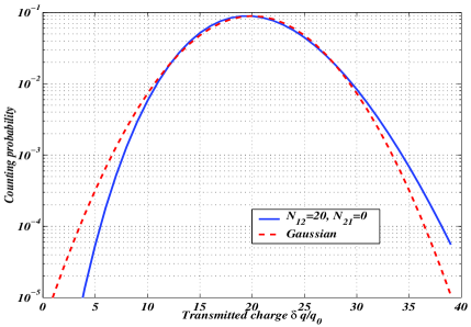
FIG. 1.: The third moment (5) determines the shape of the distribution $P(q)$, namely its skewness. This is illustrated by a distribution of the form (1) and a Gaussian with the same mean and variance. For $C_{3}>0$ the peak is somewhat more stretched to the right than to the left.

The meaning of Eq. (6) is similar to that of the Schottky formula for the second correlator ${\cal P}=2\langle\!\langle\delta q^{2}\rangle\!\rangle=2e^{\ast}I$ which is usually used to determine the effective charge $e^{\ast}$ from the tunneling current noise. The Schottky formula is valid when charge flow is unidirectional, which means $m_{12}\gg m_{21}$ (see Eq. (3)). The latter can be true only at sufficiently low temperatures $k_{\rm B}T\ll eV$. This requirement of a cold sample at a relatively high bias voltage is the origin of a well known difficulty in the noise measurement. In contrast, the relation (6) is not constrained by any requirement on sample temperature.

On a general basis we expect the relation (6 to hold approximately even outside the tunneling regime. Indeed, for the Nyquist noise at equilibrium all odd moments vanish. Combined with the temperature independence of $P(q)$ out of equilibrium, this implies a relatively weaker dependence on $eV/k_{\rm B}T$ than in the noise power at the Nyquist-Schottky crossover. This is manifest, for instance, in the temperature independent first moment of $P(q)$ for free fermions (the Landauer formula).

This property of the third moment, if confirmed experimentally, may prove to be quite useful for determining the quasiparticle charge. In particular, this applies to the situations when the $I-V$ characteristic is strongly nonlinear, when it is usually difficult to unambiguously interpret the variation of the second moment with current as a shot noise effect or as a result of thermal noise modified by non-linear conductance. We stress that this is a completely general problem pertinent to any interacting system. Namely, in systems such as Luttinger liquids, the $I-V$ nonlinearities arise at $eV\geq k_{\rm B}T$. However, it is exactly this voltage that has to be applied for measuring the shot noise in the Schottky regime.

Now we turn to the derivation of the main result (1). The starting point of our analysis will be the tunneling Hamiltonian $\hat{\cal H}=\hat{\cal H}_{1}+\hat{\cal H}_{2}+\hat{V}$, where $\hat{\cal H}_{1,2}$ describe the leads and $\hat{V}=\hat{J}_{12}+\hat{J}_{21}$ is the tunneling operator. The specific form of the operators $\hat{J}_{12}$, $\hat{J}_{21}$ that describe tunneling of a quasiparticle between the leads will be unimportant for the most of our discussion.

The counting statistics generating function $\chi(\lambda)$ can be written [16] as a Keldysh partition function

$$\chi(\lambda)=\Big{\langle}{\rm T}_{\rm K}\exp\left(-i\int_{C_{0,\tau}}\hat{\cal H}_{\lambda}(t)dt\right)\Big{\rangle},$$ (7)

where a counting field $\lambda(t)$ is added to the phase of the tunneling operators $\hat{J}_{12}$, $\hat{J}_{21}$ as

$$\hat{V}_{\lambda}=e^{\frac{i}{2}\lambda(t)}\hat{J}_{12}(t)+e^{-\frac{i}{2}\lambda(t)}\hat{J}_{21}(t)$$ (8)

Here $\lambda(t)=\pm\lambda$ is antisymmetric on the forward and backward parts of the Keldysh contour $C_{0,\tau}\equiv\left[0\to\tau\to 0\right]$. Eqs. (7), (8) originate from the analysis of a coupling Hamiltonian for an ideal “passive charge detector” without internal dynamics [16, 24].

In what follows we compute $\chi(\lambda)$ and establish a relation with the Kubo theorem for tunneling current [29]. For that, we perform the usual gauge transformation turning the bias voltage into the tunneling operator phase factor as $\hat{J}_{12}\rightarrow\hat{J}_{12}e^{-ieVt}$, $\hat{J}_{21}\rightarrow\hat{J}_{21}e^{ieVt}$. Passing to the Keldysh interaction representation, we write

$$\chi(\lambda)=\Big{\langle}{\rm T}_{\rm K}\exp\left(-i\int_{C_{0,\tau}}\hat{V}_{\lambda(t)}(t)dt\right)\Big{\rangle}$$ (9)

Diagrammatically, the partition function (9) is a sum of linked cluster diagrams with appropriate combinatorial factors. To the lowest order in the tunneling operators $\hat{J}_{12}$, $\hat{J}_{21}$ we only need to consider linked clusters of the second order. This gives $\chi(\lambda)=e^{W(\lambda)}$, where

$$W(\lambda)=-\frac{1}{2}\int\!\!\int_{C_{0,\tau}}\!\Big{\langle}{\rm T}_{\rm K}\hat{V}_{\lambda(t)}(t)\hat{V}_{\lambda(t^{\prime})}(t^{\prime})\Big{\rangle}\,dtdt^{\prime}$$ (10)

There are several different contributions to this integral, from $t$ and $t^{\prime}$ on the forward or backward parts of the contour $C_{0,\tau}$. Evaluating them separately, we obtain

$$W(\lambda)=\int_{0}^{\tau}\!\!\int_{0}^{\tau}\!\Big{\langle}\hat{V}_{-\lambda}(t)\hat{V}_{\lambda}(t^{\prime})\Big{\rangle}\,dt^{\prime}dt$$ (11)

$$-\!\int_{0}^{\tau}\!\!\int_{0}^{t}\!\!\Big{\langle}\!\hat{V}_{\lambda}(t)\hat{V}_{\lambda}(t^{\prime})\!\Big{\rangle}\,dt^{\prime}\!dt-\!\int_{0}^{\tau}\!\!\int_{t}^{\tau}\!\!\Big{\langle}\!\hat{V}_{-\lambda}(t)\hat{V}_{-\lambda}(t^{\prime})\!\Big{\rangle}\,dt^{\prime}\!dt$$ (12)

We substitute the form (8) into Eq.(11) and average by pairing $\hat{J}_{12}$ with $\hat{J}_{21}$. This gives

$$W(\lambda)=(e^{i\lambda}\!-\!1)N_{1\to 2}(\tau)+(e^{-i\lambda}\!-\!1)N_{2\to 1}(\tau)$$ (13)

$${\rm with}\quad N_{a\to b}=\int_{0}^{\tau}\!\!\int_{0}^{\tau}\langle\hat{J}_{ba}(t)\hat{J}_{ab}(t^{\prime})\rangle\,dtdt^{\prime}$$ (14)

Exponentiating (13) gives the result (1)

It is instructive to relate the quantities (14) with the Kubo theorem. We consider the tunneling current operator $\hat{\cal I}(t)=-ie^{\ast}\left(\hat{J}_{12}(t)-\hat{J}_{21}(t)\right)$. From the Kubo theorem for the tunneling current [29], the mean integrated current $\int_{0}^{\tau}\langle\hat{\cal I}(t)\rangle dt$ scaled by $e^{\ast}$ is nothing but

$$\int_{0}^{\tau}\!\!\int_{0}^{\tau}\Big{\langle}\left[\hat{J}_{21}(t),\hat{J}_{12}(t^{\prime})\right]\Big{\rangle}\,dtdt^{\prime}=N_{1\to 2}-N_{2\to 1}$$ (15)

By writing $N_{a\to b}=m_{ab}\tau$, we obtain the first relation (4). To obtain the second relation (4) we consider the variance of the charge transmitted in time $\tau$. It is given by a time integral of an averaged symmetrized product of two current operators [28]

$$\langle\!\langle\delta q^{2}\rangle\!\rangle=(e^{\ast})^{2}\int_{0}^{\tau}\!\!\int_{0}^{\tau}\Big{\langle}\left\{\hat{\cal I}(t),\hat{\cal I}(t^{\prime})\right\}_{+}\Big{\rangle}\,dtdt^{\prime}$$ (16)

The integral in (16) can be rewritten as

$$\int_{0}^{\tau}\!\!\int_{0}^{\tau}\!\Big{\langle}\!\left\{\hat{J}_{12}(t),\hat{J}_{21}(t^{\prime})\right\}_{+}\!\Big{\rangle}\,dtdt^{\prime}=N_{1\to 2}\!+\!N_{2\to 1}$$ (17)

which immediately leads to (4).

The result (1), and thereby the formula (6) for the 3-rd correlator, are valid only at low transmission. In that the situation is similar to the Kubo formula for the tunneling current, which is valid only in the tunneling Hamiltonian approximation. To illustrate this we recall the expression for counting statistics for a single channel noninteracting Fermi system (point contact) in the presence of a dc voltage $V$ and temperature $T$ [16],

$$\chi(\lambda)=\exp\left(-N_{T}{\cal U}_{+}{\cal U}_{-}\right),\quad N_{T}=\frac{\tau k_{\rm B}T}{2\pi\hbar}$$ (18)

$${\cal U}_{\pm}\!={\cal U}/2\pm\cosh^{-1}\!\left(t\cosh({\cal U}/2+\!i\lambda)+\!r\cosh\left({\cal U}/2\right)\right)$$ (19)

where $\tau$ is a measurement time, and ${\cal U}=eV/k_{\rm B}T$. This result holds for any values of the transmission and reflection constants $t$ and $r$ (constrained by $t+r=1$). The formula (18) was obtained in Ref. [16] by explicitly evaluating the Keldysh partition function in the scattering basis representation.

The 3-rd correlator $\langle\!\langle\delta q^{3}\rangle\!\rangle$ can be obtained from (18) by expanding $\ln\chi(\lambda)$ in Taylor series up to $O(\lambda^{3})$:

$$\langle\!\langle\delta q^{3}\rangle\!\rangle=e^{3}t(1-t)N_{T}\left(6t\frac{\sinh{\cal U}-{\cal U}}{\cosh{\cal U}-1}+(1-2t){\cal U}\right)$$ (20)

This expression is a function of the bias-to-temperature ratio ${\cal U}$, and so in this case the relation (20) for the 3-rd correlator does not hold (see Fig. 2). Asymptotically

$$\langle\!\langle\delta q^{3}\rangle\!\rangle=\cases{e^{2}(1-t)I\tau,\quad&$eV\ll k_{\rm B}T$\cr e^{2}(1-2t)(1-t)I\tau,\quad&$eV\gg k_{\rm B}T$}$$ (21)

where $I=\frac{e^{2}}{2\pi\hbar}tV$. One can also average over the universal Dorokhov’s distribution of transmission in a multichannel mesoscopic metal [18] (see Fig. 2).

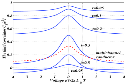
FIG. 2.: The third correlator $C_{3}$ scaled by $e^{2}I$, with $I$ the time-averaged current [see Eqs. (5), (6)], for the single channel problem (18), (20), and for a phase-coherent mesoscopic multichannel conductor. Note that the relation $C_{3}=e^{2}I$ holds approximately at not too large transmission $t$.

Eqs. (20), (21) indicate nonuniversality of the relation (6) outside the tunneling regime. They also lead to an interesting qualitative prediction: At $t>0.5$ the ratio $\langle\!\langle\delta q^{3}\rangle\!\rangle/I$ can become negative. Such a signature could be observed even if it proves difficult to measure $\langle\!\langle\delta q^{3}\rangle\!\rangle$ quantitatively with sufficient precision. This is important in view of the difficulties in measuring the counting statistics (see below).

In the single channel problem (18) the tunneling regime is realized at low transmission $t$. To connect with the results (1), (6) we analyze the expression (18) at $t\ll 1$. To the lowest order in small $t$ we have

$${\cal U}_{+}={\cal U},\quad{\cal U}_{-}=t\frac{e^{{\cal U}}\left(e^{i\lambda}-1\right)+\left(e^{-i\lambda}-1\right)}{e^{\cal U}-1}$$ (22)

Substituting this in Eq.(18) we recover (1) with

$$N_{2\to 1}(\tau)=\frac{eV\tau}{2\pi\hbar}\frac{t}{e^{\cal U}-1},\quad N_{1\to 2}(\tau)=e^{\cal U}N_{2\to 1}(\tau)$$ (23)

the rates of two Poisson processes.

The measurement of the distribution $P(q)$ is a nontrivial task. Current fluctuations must be amplified with a very low noise preamplifier (e.g. the one used in Refs. [8, 10]). Amplified signal can then be digitized and analyzed with computer. This setup in principle allows to reconstruct the full statistics of transmitted charge. In practice, however, the correlators of high order become increasingly difficult to extract.

The main source of error in the measurement of the $k$-th cummulant $C_{k}$ of the distribution $P(q)$ is statistical. The nongaussian character of the amplifier noise does not present a problem, since the mean time-averaged value of the $k$-th cummulant $C_{k}^{(a)}$ for the amplifier can be subtracted if known with sufficient accuracy. The measured value $C_{k}$ should be compared to (i) the variance ${\rm var\ }C_{k}$ of the $k$-th cummulant statistics and (ii) the variance ${\rm var\ }C_{k}^{(a)}$ of the $k$-th cummulant of the amplifier noise. The variance is in both cases expressed through the correlators of order $2k$. The correlators of even order for a generic distribution can be estimated, by virtue of the central limit theorem, using Gaussian statistics:

$${\rm var\ }C_{k}=\left(\langle\delta q^{2k}\rangle\right)^{1/2}\simeq\left((2k-1)!!\,\langle\delta q^{2}\rangle^{k}\right)^{1/2}$$ (24)

Fluctuations introduced by amplifier can also be estimated using Gaussian statistics. For the amplifier noise of spectral density $A$ (measured in ${\rm A^{2}/Hz}$), charge fluctuations are $\delta Q^{2}=\frac{1}{2}A\tau$, where $\tau$ is sampling time. An estimate of the variance ${\rm var\ }C_{k}^{(a)}$, similar to Eq.(24), gives

$${\rm var\ }C_{k}^{(a)}=\left((2k-1)!!\left({\textstyle\frac{1}{2}}A\tau\right)^{k}\right)^{1/2}$$ (25)

For odd $k$ the commulant $C_{k}=\langle\!\langle\delta q^{k}\rangle\!\rangle$ mean value is proportional to the current $I$, as discussed above. The fluctuations due to the amplifier are independent of $I$. In the Nyquist regime (at small $I$) the variance ${\rm var\ }C_{k}$ is independent on $I$ and is determined by thermal noise. In the Schottky noise regime (at large $I$) the fluctuations are determined by $I$, and ${\rm var\ }C_{k}\propto I^{k/2}$. Therefore at $k>2$ one can increase the signal-to-noise ratio by increasing the current until ${\rm var\ }C_{k}\approx{\rm var\ }C_{k}^{(a)}$

In the shot noise regime, when $\langle\delta q^{2}\rangle=eI\tau\approx A\tau$, we can estimate the signal-to-noise ratio as

$$S/N\simeq\frac{\langle\!\langle q^{k}\rangle\!\rangle}{2{\rm var\ }C_{k}}\simeq\frac{1}{2((2k-1)!!)^{1/2}}\left(\frac{2e^{2}}{A\tau}\right)^{k/2-1}$$ (26)

It is clear from Eq.(26) that it is beneficial to decrease the sampling time $\tau$ to gain sensitivity. Estimates for typical values of $A=10^{-28}~{}{\rm A^{2}/Hz}$ and $\tau=10^{-7}~{}{\rm s^{-1}}$ give for the $k=3$ commulant $S/N\approx 10^{-2}$. This value is acceptable, since repeating the measurement many times over a long time $\cal T$ and averaging will further reduce statistical fluctuations by a factor of $\sqrt{\cal T/\tau}$. For the cummulants of higher order $k>3$ the situation is more problematic.

In summary, the counting statistics (1) of tunneling current is found to be universal and independent of the character of interactions. For the third correlator we obtain a generalized Schottky formula (6). This formula is valid at both large and small $eV/k_{\rm B}T$ and can be used to measure quasiparticle charge at temperatures $k_{\rm B}T\geq eV$. A method for measuring the third correlator is proposed.

This research is supported by the Binational Science Foundation and by the MRSEC Program of the National Science Foundation under Grant No. DMR 98-08941.

REFERENCES

- [1] G. B. Lesovik, JETP Lett. 49, 592 (1989)
- [2] V. K. Khlus, Sov. Phys. JETP 66, 1243 (1987)
- [3] M. Buttiker, Phys. Rev. Lett. 65, 2901 (1990)
- [4] C. W. J. Beenakker and M. Buttiker, Phys. Rev. B46, 1889 (1992)
- [5] C. L. Kane and M. P. A. Fisher, Phys. Rev. Lett. 72, 724 (1994)
- [6] M. Reznikov, M. Heiblum, Hadas Shtrikman and D. Mahalu, Phys. Rev. Lett. 75, 3340 (1995);
- [7] A. Kumar, L. Saminadayar, D. C. Glattli, Y. Jin and B. Etienne, Phys. Rev. Lett. 76, 2778 (1996)
- [8] R. de-Picciotto, M. Reznikov, M. Heiblum, V. Umansky, G. Bunin and D. Mahalu, Nature 389, 162 (1997);
- [9] L. Saminadayar, D. C. Glattli, Y. Jin and B. Etienne, Phys. Rev. Lett. 79, 2526 (1997)
- [10] M. Reznikov, R. de Picciotto, T. G. Griffiths, M. Heiblum, and V. Umansky, Nature 399, 238 (1999)
- [11] T. G. Griffiths, E. Comforti, M. Heiblum, A. Stern, V. Umansky, Phys. Rev. Lett. 85, 3918 (2000)
- [12] A. Steinbach, J. M. Martinis, M. H. Devoret, Phys. Rev. Lett. 76, 2778 (1996)
- [13] R. J. Schoelkopf, P. J. Burke, A. A. Kozhevnikov, D. E. Prober, Phys. Rev. Lett. 78, 3370 (1997)
- [14] R. J. Schoelkopf, A. A. Kozhevnikov, D. E. Prober, M. Rooks, Phys. Rev. Lett. 80, 2437 (1998)
- [15] L. S. Levitov, G. B. Lesovik, JETP Lett. 58, 230 (1993);
- [16] L. S. Levitov, H. W. Lee, G. B. Lesovik, J. of Math. Phys. 37, 4845 (1996); L. S. Levitov and G. B. Lesovik, “Quantum Measurement in Electric Circuit,” cond-mat/9401004
- [17] D. A. Ivanov, L. S. Levitov, JETP Lett. 58, 461 (1993)
- [18] H. W. Lee, L. S. Levitov, A. Yu. Yakovets, Phys. Rev. B51, 4079 (1995)
- [19] Yu. V. Nazarov, cond-mat/9908143, Ann. Phys. (Leipzig) 8, SI-193 (1999)
- [20] D. A. Ivanov, H. W. Lee, L. S. Levitov, Phys. Rev. B56, 6839 (1997)
- [21] B. A. Muzykantskii, D. E. Khmelnitskii, Phys. Rev 50, 3982 (1994)
- [22] W. Belzig, Yu. V. Nazarov, Phys. Rev. Lett. 87, 067006 (2001)
- [23] G. B. Lesovik and R. Loosen, JETP Lett. 65, 295 (1997)
- [24] Yu. V. Nazarov, M. Kindermann, “Full counting statistics of a general quantum mechanical variable,” condmat/0107133
- [25] C. W. J. Beenakker, H. Schomerus, Phys. Rev. Lett. 86, 700 (2001)
- [26] A. V. Andreev and A. Kamenev, Phys. Rev. Lett. 85 1294 (2000)
- [27] The relation between cummulants and correlators is generally more complicated than Eq.(5) for the third cummulant. For example, .
- [28] E. V. Sukhorukov, D. Loss, “Shot noise of weak cotunneling current: Non-equilibrium fluctuation-dissipation theorem,” cond-mat/0106307
- [29] G. D. Mahan, “Many-Particle Physics,” (Plenum Press, 1981): Sec. 9.3