Vortex phases

Abstract

These lecture notes are meant to provide a pedagogical introduction, and present the latest theoretical and experimental developments on the physics of vortices in type II superconductors.

1 Why and what in vortices

The discovery of high Tc superconductors has shattered the comforting sense of understanding that we had of the phase diagram and physical properties of type II superconductors, and in particular of the mixed (vortex) phase in such systems. Indeed, it was well known since Abrikosov abrikosov_vortex_first that above $H_{c1}$ the magnetic field penetrates under the form a vortex, made of a filament of radius $\xi$ (the coherence length) surrounded by supercurrent screening the external field running over a radius $\lambda$ (the penetration length). Because of the repulsion between vortices due to supercurrents (see Fig. 1), the naive idea is that vortex will form a perfect triangular crystal (the Abrikosov lattice). This has led to the phase diagram shown in Fig. 1, that has been the cornerstone of our understanding of all type II superconductors for more than three decades tinkham_book_superconductors ; DeGennes_supra . However in high Tc, one could reach much higher temperatures, and it was soon apparent that some of the physics linked to the existence of the thermal fluctuations and disorder was overlooked. This led to a burst of investigations, both theoretical and experimental, to understand the physical properties of such vortex matter. Of course, high Tc were not the only field of investigations and low Tc superconductors were reexamined as well, now that we knew what to look for in them.

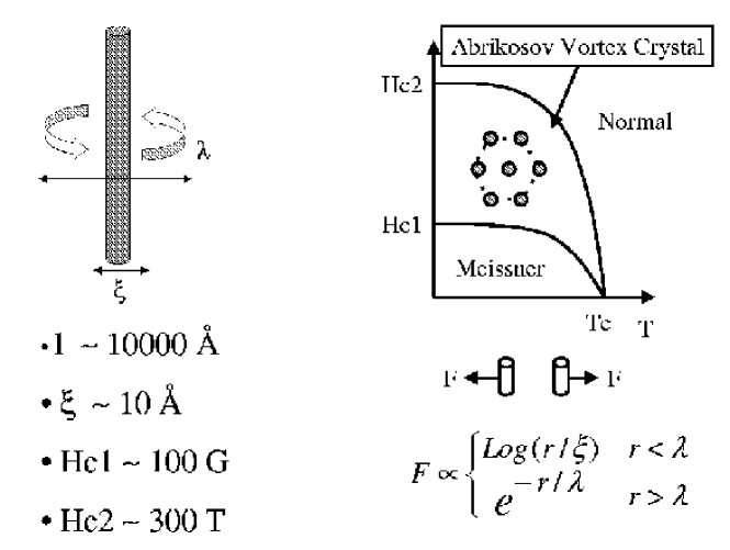
Figure 1: The structure of a vortex, with a core size $\xi$ and supercurrent running over a radius $\lambda$ the penetration length. Typical values for high Tc are given. Due to supercurrents vortex repel with a force $F$. This leads to the naive phase diagram where a crystal of vortex exists between $H_{c1}$ and $H_{c2}$.

Indeed the vortex phase provides an excellent system for both the fundamental researcher and one in search of physics with useful applications. From the fundamental point of view, vortex matter provides a unique system where one can study a crystal, in which one can vary the density (the lattice spacing) at the turn of a knob (simply by varying the magnetic field). In addition, because this crystal is embedded in a “space” with a much finer lattice constant (the real atomic crystal), it can be submitted to various perturbations such as disorder, difficult to investigate in normal crystals. This provides thus a unique opportunity to study the combined effect of disorder and thermal fluctuations on a crystal. From a more practical point of view, if one has vortices in a superconductor and passes a current $J$ in them, the current will act as a force on the magnetic tubes that are the vortices, and they will start to slide. The sliding in turn generates an electric field $E$, which means that the superconductor is not superconducting any more, due to the motion of vortices (see Fig. 2).

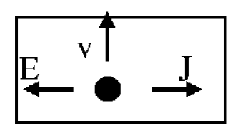
Figure 2: A current $J$ driven in a superconductor exert a force on the vortices, making them slide sideways with a velocity $v$. Since the vortices are flux tubes this generates an electric field $E$ in the direction of the current and thus to a finite (and rather bad) resistance.

The resistance is rather poor and is simply $\rho=\rho_{n}(H/H_{c2})$ (Bardeen-Stephen resistance). In order to get a good superconductor, it is thus necessary to prevent the vortices from moving by pinning them. Hence the strong practical incentive to understand the properties (both static and dynamics) of vortices in the presence of disorder.

A study of vortices prompts for several questions, that we will try to address in these notes:

• What is the effect of disorder on the Abrikosov vortex crystal ?

• How to describe the vortex phase ? Does one needs the full Ginzburg-Landau description or can one use a simplified description modelling vortices as elastic spaghettis ?

• What is the phase diagram and the static physical properties of the vortices in presence of disorder and thermal fluctuations ?

• What are the dynamical properties ? Is there a linear response and more generally what is the $I-V$ characteristics ?

• What is the nature of the vortex system when it is in motion ?

• Are there links with other physical systems exhibiting the same competition between crystal order and disorder ?

Of course, these questions have been examined intensively in the last 30 years, and represent an impressive body of research work. So in these few pages we have to make a choice. Reviews already exist on vortices blatter_vortex_review ; brandt_review_superconductors ; giamarchi_book_young ; nattermann_vortex_review so we will try to present in these notes the basic ideas enabling the reader to understand the concept behind the variety of studies, and then bring the reader up to date with the recent theoretical and experimental developments that are left out of the previous reviews. The plan of the paper is as follows: in Section 2 we discuss an elastic description of the vortices, and the issue of lattice melting. In Section 3 we discuss the effects of disorder, introduce the basic lengthscales and physical concepts and discuss the limitations of the previously proposed solutions to tackle this problem. In Section 4 we discuss the recent theory of the Bragg glass and compare it with the host of experimental data on the statics of the vortex lattice. In Section 5 we discuss the more complicated issue of the dynamics. Finally conclusions, perspectives and contact with other physical systems can be found in Section 6.

2 Elastic description of vortices

A way to get a tractable description of the vortex lattice is to ignore the microscopic aspects of the superconducting state and the Ginzburg-Landau description of the vortex, and simply consider the vortices as an elastic object. The core is like a piece of string and the supercurrents provide the repulsive (elastic) forces. Of course such a description is a simplification and depending on the problem, it will be necessary to check that important physics has not been left out in the process. However, such a description has the advantage of being simple enough so that additional effects such as disorder can be included, and retains in fact most of the interesting physics for amacroscopic description of the vortex lattice (phase diagram, imaging, transport). Another advantage is that this allows us to make contact with a large body of related problems as will be discussed in section 6.

We thus describe the vortex system as objects having an equilibrium position $R_{i}^{0}$ (on a triangular lattice for the vortices, but this is of course general) and a displacement $u_{i}$ compared to this equilibrium position. $u_{i}$ is a vector with a certain number $n$ of components. The vortices being lines $n=2$, since displacements are on the plane perpendicular to the $z$ axis. The elastic Hamiltonian is

$$H=\frac{1}{2\Omega}\sum_{\alpha\beta}\sum_{q}c_{\alpha\beta}(q)u_{\alpha}(q)u_{\beta}(-q)$$ (1)

where $\alpha=x,y,z$ are the spatial coordinates. The $c_{\alpha\beta}(q)$ are the elastic constants. The fact that they have a non trivial dependence on $q$ comes from the long range nature of the forces between the vortices. The $c$ can be computed from the microscopic forces between vortices. Standard elasticity corresponds to $c(q)=cq^{2}$. Such a behavior will always be correct at large distance (small $q$) since the forces have a finite range $\lambda$. In (1) various physical process have in principle to be distinguished and correspond to different elastic constants. This corresponds to bulk, shear and tilt deformations of the vortex lattice as shown on Fig. 3.

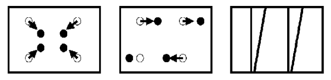
Figure 3: Three different deformations of the vortex lattice (compression (bulk), shear and tilt) correspond to three different elastic constants, respectivelly called $c_{11}$, $c_{66}$ and $c_{44}$.

Although these different elastic constants can be widely different in magnitude (for example bulk compression is usually much more expensive than shear), this is a simple practical complication that does not change the quadratic nature of the elastic Hamiltonian. Such a description is of course also valid for anisotropic superconductors (such as the layered High Tc ones), provided that the anisotropy is not too large. If the material is too layered then it is better to view the vortices as pancakes living in each plane and coupled by Josephson or electromagnetic coupling between the planes as shown in Fig. 4.

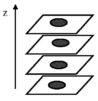
Figure 4: In very anisotropic materials, it is best to see a vortex line as a stack of pancakes vortices coupled by electromagnetic or Josephson coupling. For most cases however a line description will be sufficient.

For moderately anisotropic materials viewing the stack of pancakes as a vortex line is however enough. In this notes we will stick to this description.

The melting of the vortex lattice can easily be extracted from the elastic description. Although a detailed theory of melting is still lacking, one can use a basic criterion, known as Lindemann criterion that states that the crystal melts when the thermally induced displacements a particle in the crystal becomes some sizeable fraction of the lattice spacing. On a more formal level the melting is given by

$$\langle u^{2}\rangle=l_{T}^{2}=C_{L}^{2}a^{2}$$ (2)

which defined the “effective” (thermal) size of the particle (also known as Lindemann length). The proportionality constant that reproduces correctly the melting is empirically determined to be $C_{L}\sim 0.1-0.2$. A simple calculation based on the elastic the elastic description thus gives

$$\frac{T_{m}}{c}=C_{L}^{2}a^{2}$$ (3)

showing that the melting temperature goes down as the lattice spacing goes down (or the magnetic field up). Of course the full quantitative study for the vortex lattice should be done with the full fledged elastic Hamiltonian (including bulk, shear, tilt), but the main conclusions remain unchanged houghton_fusion_vortex ; nelson_fusion_vortex . This leads to the first modification of the naive Abrikosov phase diagram taking into account the melting shown in Fig. 5.

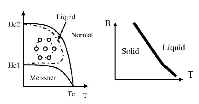
Figure 5: Thermal fluctuations induce melting of the vortex lattice. On the left the full melting curve is shown. For high Tc, in practice one is often far from both $H_{c1}$ and $H_{c2}$ leading to the apparent phase diagram shown on the right.

Close to $H_{c1}$ the elastic constants drop down (since the vortices get separated by more than $\lambda$ the force between them is exponentially small), and from (3) the crystal also melts, leading the reentrant behavior shown in Fig. 5.

Early experimental studies charalambous_melting_rc ; safar_tricritical_prl ; safar_transport_tricritical ; kwok_vortex_melting of the melting transition were based on transport measurements. The sudden onset of an ohmic resistance was argued to signify melting and its location in the (H,T) space is the locus of the melting phase boundary. Typical experimental results are shown in Fig. 6, where the onset is characterized by a pronounced knee in the resistance.

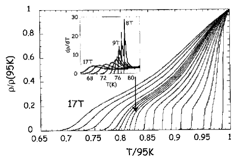
Figure 6: T-dependence of ohmic resistance at various field values. The sudden onset marked by a pronounced knee marks the melting transition. The inset shows a plot of the temperature derivative of the resistance which, surprisingly mimics the specific heat jump across the transition kwok_vortex_melting

With increasing external field, the onset moves to lower temperatures and eventually broadens considerably. This implies that at sufficiently large fields, the sharp first order transition crosses over to a more continuous second order like transition, an effect expected to be the result of disorder (see later). At lower fields and higher temperatures, the melting transition is closely approximated by the disorder-free case, discussed above. Later experiments performed on thermodynamic quantities such as the magnetization and specific heat confirmed the first order nature of the melting transition, at least for weak disorder. Fig. 7 shows an experimental phase diagram of BSCCO obtained by local magnetization using a novel hall-bar technique zeldov_diagphas_bisco .

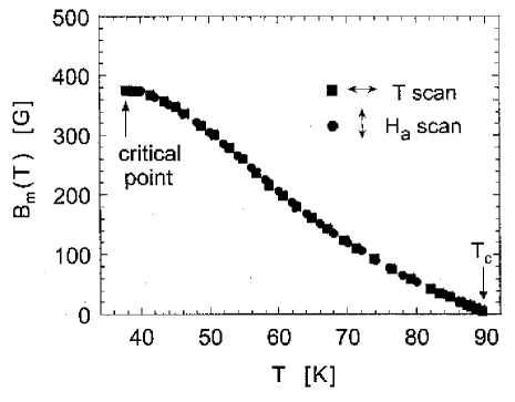
Figure 7: Melting phase diagram obtained from the jump in local induction for both isothermal and isofield data zeldov_diagphas_bisco . Note the similarity of the phase boundary with theoretical expectations in Fig. 5 above.

Figure 8 shows typical measurements of the jump in the local induction across this transition, by either changing temperature at a fixed field or changing field at a fixed temperature.

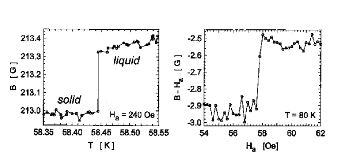
Figure 8: Typical jumps in local induction for isothermal and isofield measurements from Hall bar method zeldov_diagphas_bisco . Both the solid and liquid phases have no measurable pinning in the bulk and the data are reversible.

In both cases, a positive jump in $B$ is observed in going from the solid to the liquid phase. Using the Clapeyron- equation :

$$\frac{dH_{m}}{dT}=-\frac{\Delta S}{\Delta M}$$ (4)

where $\Delta S$ is the entropy change and $\Delta M$ is the change in magnetization (density of vortices). The experimental phase diagram is consistent with theoretical expectations as shown in Fig. 5 above. The negative slope of the melting curve is consistent with an increase of density in the liquid phase, curiously akin to a “water-like” melting phenomenon. Very little experimental work is available on the low field reentrant branch of the melting phase boundary. At low fields the intervortex interaction is weak and the effects of disorder dominate. Reentrant phenomena in peak effect (see Section 4.4) have been somewhat widely observed and is thought to be dominated by effects of disorder, rather than thermal fluctuations.

Finally, besides the phase diagram, what are the physical quantities that one can in principle compute and that are directly connected to experiments ? The first important information is the relative displacements correlation function

$$B(r)=\overline{\langle[u(r)-u(0)]^{2}\rangle}$$ (5)

where $\langle\rangle$ is the average over thermal fluctuations and $\overline{\cdots}$ is the average over disorder (if need be). (5) indicates how the displacements between two points in the system separated by a distance $r$ grow (see Fig. 9).

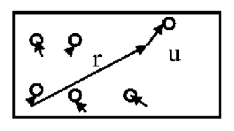
Figure 9: The relative displacement correlation function $B(r)$ measuring the displacements between two points separated by a distance $r$ is directly measured in experiments such as decoration experiments.

Decoration experiments provide a direct measure of this correlation function as we will see. In a perfect crystal $B(r)=0$, whereas both thermal fluctuations and disorder will make the displacements grow. How $B(r)$ grows tells us whether the system is well ordered or not. In a good crystal $B(r)$ will saturate to a finite value whereas it will grow unboundedly if the perfect positional order of the crystal is destroyed.

Another important quantity, directly measures in diffraction experiments is the structure factor

$$S(q)=\overline{\langle\rho(q)\rho(-q)\rangle}$$ (6)

In a perfect crystal this consists of Bragg peaks at the vectors $K$ of the reciprocal lattice of the crystal. If one considers one such peak its shape (as shown on Fig. 10)

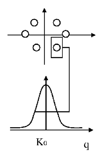
Figure 10: The structure factor measured in diffraction experiments such as neutrons or X-rays. The shape of a peak is given by the Fourier transform of the positional correlation function $C(r)$ (see text).

is the Fourier transform of the positional correlation function

$$C(r)=\overline{\langle e^{iKu(r)}e^{-iKu(0)}\rangle}$$ (7)

Thus in a perfect crystal $C(r)=1$ and the Fourier transform is a $\delta(q)$ Bragg peak. If there are only thermal fluctuations $C(r\to\infty)\to{\rm Cste}$ (in fact $C(\infty)=e^{-K^{2}l_{T}^{2}/2}$). The Fourier transform is still a $\delta$ peak but with a reduced weight which is simply the Debye Waller factor. The faster $C(r)$ decreases the more disordered is the crystal. If $C(r)$ decreases exponentially to zero with a characteristics lengthscale $R_{a}$, the peak in the structure factor is some patatoidal (lorentzian like) shape with a width $R_{a}^{-1}$ indicating that the perfect translational order is lost. Although it is not always true (it is only true for gaussian fluctuations such as thermal fluctuations) a rule of thumb is

$$C(r)\sim e^{-K^{2}B(r)/2}$$ (8)

showing quite logically that the faster the relative displacements grow the more positional order (measured by the Bragg peaks) is destroyed in the system.

3 Disorder, basic lengths and open questions

The next task is to consider the effects of disorder. In real systems, disorder exists in all varieties in the underlying atomic crystal: vacancies, interstitials, lattice dislocations, grain boundaries, twin boundaries, second-phase precipitates, etc. In high quality single crystals it is possible to limit dominant disorder to point like impurities. Additionally, point like disorder can be, and sometimes is, intentionally added to systems in the form of electron irradiation in the case of the cuprates and/or substitutional atomic impurities of various kinds in low Tc systems. More artificial disorder can be introduced for example by heavy ions irradiation that produce columns of defects in the material. We will briefly mention the consequences of such artificial disorder in Section 6, but most of these notes will be devoted to the effects of point like impurities.

Such impurities (as shown on Fig. 11)

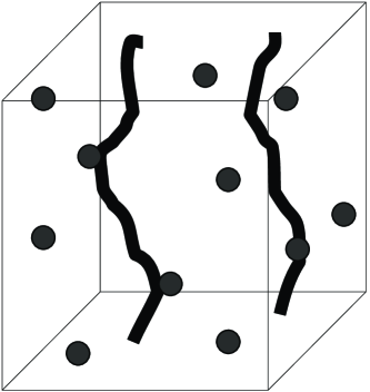
Figure 11: Point like impurities (small circles) act as pinning centers for the vortices.

can be modeled by a random potential $V(r)$ coupled directly to the density $\rho(r)=\sum_{i}\delta(r-R^{0}_{i}-u_{i})$ of vortex lines

$$H_{dis}=\int d^{d}rV(r)\rho(r)$$ (9)

In principle one has “just” to add (9) to (1) and solve. Unfortunately the coupling of the displacements to disorder is highly non linear (since it occurs inside a $\delta$ function), and thus this is an horribly complicated problem. Physically this traduces the fact that there is a competition between the elastic forces that want the system perfectly ordered and the disorder that let the lines meander. This competition is bound to lead to complicated states where the system tries to compromise between these two opposite tendencies.

In order to understand the basic physics of such problem a simple (but ground breaking !) scaling argument was put forward by Larkin larkin_70 . To know whether the disorder is relevant and destroys the perfect crystalline order, let us assume that there exists a characteristic lengthscale $R_{a}$ for which the relative displacements are of the order of the lattice spacing $u(R_{a})-u(0)\sim a$. If the displacements vary of order $a$ over the lengthscale $R_{a}$ the cost in elastic energy from (1) is

$$\frac{c}{2}R_{a}^{d-2}a^{2}$$ (10)

by simple scaling analysis. Thus in the absence of disorder minimizing the energy would lead to $R_{a}=\infty$ and thus to a perfect crystal. In presence of the disorder the fact that displacements can adjust to take advantage of the pinning center on a volume of size $R_{a}^{d}$ allow to gain some energy. Since $V$ is random the energy gained by adapting to the random potential is the square root of the potential over the volume $R_{a}^{d}$, thus one gains an energy from (9)

$$-VR_{a}^{d/2}\rho_{0}$$ (11)

Thus minimizing (10) plus (11) shows that below four dimensions the disorder is always relevant and leads to a finite lengthscale

$$R_{a}\sim a\left(\frac{c^{2}a^{d}}{V^{2}\rho_{0}^{2}}\right)^{1/(4-d)}$$ (12)

at which the displacements are of order $a$. The conclusion is thus that even an arbitrarily weak disorder destroys the perfect positional order below four dimensions, and thus no disordered crystal can exist for $d\leq 4$. This is an astonishing result, which has been rediscovered in other context (for charge density waves $R_{a}$ is known as Fukuyama-Lee fukuyama_pinning length and for random field Ising model this is the Imry-Ma length imry_ma ). Of course it immediately prompt the question of what is the resulting phase of elastic system plus disorder ?

Since solving the full problem is tough another important step was made by Larkin larkin_70 ; larkin_ovchinnikov_pinning . For small displacements he realized that (9) could be expanded in powers of $u$ leading to the simpler disorder term

$$H_{\rm larkin}=\int d^{d}rf(r)u(r)$$ (13)

where $f(r)$ is some random force acting on the vortices. Because the coupling to disorder is now linear in the displacements the Larkin Hamiltonian is exactly solvable. Taking a local random force $\overline{f(r)f(r^{\prime})}=\Delta\delta(r-r^{\prime})$ gives for the relative displacements correlation function and structure factor

$$B(r) = B_{\rm thermal}(r)+\frac{\Delta}{c^{2}}r^{4-d}$$ (14)

$$C(r) = e^{-K^{2}B(r)/2}\simeq e^{-r^{4-d}}$$ (15)

where $B_{\rm thermal}$ are the displacements in the absence of disorder due to thermal fluctuations (which remain bounded in $d>2$ and are thus negligeable at large distance compared to the disorder term). Thus the solution of the Larkin model confirms the scaling analysis: (i) displacements do grow unboundedly (as a power law) and thus perfect positional of the crystal is lost; (ii) the lengthscale at which the displacements are of the order of the lattice is the similar to the one given by the scaling analysis. In addition the Larkin model tells us how fast the positional order is destroyed: the displacements grow as power law thus the positional is destroyed exponentially fast, leading to peaks in the structure factor of width $R_{a}^{-1}$. However all these conclusions should be taken with a grain of salt. Indeed the Larkin model is an expansion in powers of $u$, and thus cannot be valid at large distance (since the displacements grow unboundedly the expansion has to break down at some lengthscale). What is this characteristic lengthscale ? A naive expectation is that the Larkin model cease to be valid when the displacements are of order $a$ i.e. at $r=R_{a}$. In fact this is too naive as was noticed by Larkin and Ovchinikov. To understand why, in a transparent way, let us rewrite the density of vortices in a way more transparent than the original form

$$\rho(x)=\sum_{i}\delta(r-R_{i}^{0}-u_{i})$$ (16)

Taking the continuum limit for the displacements in (16) should be done with care since one is interested in variations of the density at scales that can be smaller than the lattice spacing. A very useful way to rewrite the density is giamarchi_vortex_short ; giamarchi_vortex_long (see also haldane_bosons ; nattermann_pinning ):

$$\rho(r)=\rho_{0}-\rho_{0}\nabla\cdot u(r)+\rho_{0}\sum_{K}e^{iK(r-u(r))}$$ (17)

which is a decomposition of the density in Fourier harmonics determined by the periodicity of the underlying perfect crystal as shown on Fig. 12.

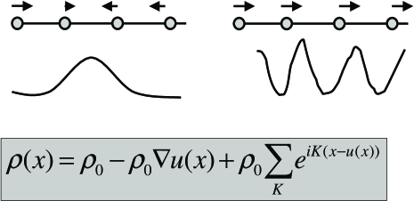
Figure 12: Various harmonics of the density. If one is only interesting in variations of the density at lengthscales large compared to the lattice spacing one has the standard “elastic” expression of the density in terms of the displacements. In the vortex system however on has to consider variations of density at lengthscales smaller than the lattice spacing and higher harmonics are needed giamarchi_vortex_short ; giamarchi_vortex_long .

The sum over the reciprocal lattice vectors $K$ obviously reproduces the $\delta$ function peaks of the density (16). If one considers particles with a given size (for vortices it is the core size $\xi$) then the maximum $K$ vector in the sum should be

$$K_{max}\sim 2\pi/\xi$$ (18)

in order to reproduce the broadening of order $\xi$ of the peaks in density. This immediately allows us to reproduce the Larkin model by expanding (9) using (17)

$$\rho_{0}\int d^{d}r\sum_{K}e^{iK(r-u(r))}V(r)$$ (19)

in powers of $u$. Clearly the expansion is valid as long as $K_{max}u\ll 1$ This will thus be valid up to a lengthscale $R_{c}$ such that $u(R_{c})$ is of the order of the size of the particles $\xi$. Note that this lengthscale is different (and quite generally smaller) than the lengthscale $R_{a}$ at which the displacements are of the order of the lattice spacing. The Larkin model cease to be valid way before the displacements become of the order of $a$ and thus cannot be used to deduce the behavior of the positional order at large length scale. In addition it is easy to check that because the coupling to disorder is linear in the Larkin model, this model does not exhibit any pinning. Any addition to an external force leads to a sliding of the vortex lattice. It thus seems that this model is not containing the basic physics needed to describe the vortex lattice. In a masterstroke of physical intuition Larkin realized that the lengthscale at which this model breaks down is precisely the lengthscale at which pinning appears larkin_ovchinnikov_pinning . The lengthscale $R_{c}$ is thus the lengthscale above which various chunks of the vortex system are collectively pinned by the disorder. A simple scaling analysis on the energy gained when putting an external force

$$H=\int d^{d}rF_{\rm ext}u(r)$$ (20)

allows to determine the critical force needed to unpin the lattice. Assuming that the critical force needed to unpin the lattice is when the energy gained by moving due to the external force is equal to the balance of elastic energy and disorder $\frac{c}{2}\xi^{2}R_{c}^{d-2}$, one obtains

$$J_{c}\propto\frac{c\xi}{R_{c}^{2}}$$ (21)

This is the famous Larkin-Ovchinnikov relation which allows to relate a dynamical quantity (the critical current at $T=0$ needed to unpin the lattice) to purely static lengthscales, here the Larkin-Ovchinikov length at which the displacements are of the order of the size of the particle. Let us insist again that this lengthscale controling pinning is quite different from the one $R_{a}$ at which displacements are of the order of the lattice spacing at that controls the properties of the positional order.

The lack of efficiency of the Larkin model to describe the behavior of displacements beyond $R_{c}$ still leaves us with the question of the nature of the positional order at large distances. However, extrapolating naively the Larkin model would give a power law growth of displacements. Such behavior is in agreement with exact solutions of interface problems in random environments (so called random manifold problems) and solutions in one spatial dimension. It was thus quite naturally assumed that an algebraic growth of displacements was the correct physical solution of the problem, and thus that the positional order would be destroyed exponentially beyond the length $R_{a}$. This led to an image of the disordered vortex lattice that consisted of a crystal “broken” into crystallites of size $R_{a}$ due to disorder. To reinforce this image (incorrect) “proofs” were given fisher_vortexglass_long to show that due to disorder dislocations would be generated at the lengthscale $R_{a}$ (even at $T=0$) further breaking the crystal apart and leaving no hope of keeping positional order beyond $R_{a}$. A summary of this (incorrect) physical image is shown on Fig. 13.

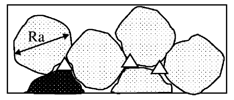
Figure 13: The (incorrect) physical image that was the commonly accepted view of what a disordered elastic system would look like. The crystal would be broken into crystallites of size $R_{a}$ by the disorder. Dislocations would be generated by the disorder at the same lengthscale.

If one believes that the positional order is lost and dislocations are spontaneously generated one can wonder whether an elastic description of the vortex lattice is a good starting point. An intermediate attitude is to consider that such a description is useful at intermediate lengthscale and can be used to obtain the pinning properties (since they are controlled by lengthscales below $R_{a}$) or as a first step in absence of a better description blatter_vortex_review . A more radical view is to consider that since positional order would be lost at large length scale it is best to ignore it from the start and that an elastic description of the vortex lattice is a bad starting point: it is much better to ignore positional order altogether and to focus on the phase of a vortex fisher_vortexglass_short ; fisher_vortexglass_long . The effect of disorder is thus introduced by a random gauge field destroying the phase coherence between the vortices. The system is then described by a random phase energy

$$H=\sum_{ij}\cos(\phi_{i}-\phi_{j}-A_{ij})$$ (22)

With certain assumptions on the properties of the gauge field (essentially that $\lambda=\infty$) the idea is that the solid vortex phase will be transformed into a glassy Gauge glass (called the vortex glass), leading to the phase diagram shown in Fig. 14.

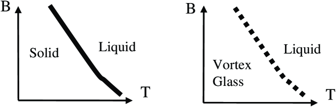
Figure 14: In a vision where positional order is ignored, and vortices are described by they phases, the solid phase is transformed into a vortex glass phase, having a continuous transition (with scaling) towards the liquid phase fisher_vortexglass_short ; fisher_vortexglass_long .

The vortex glass phase has a continuous transition, with a divergent lengthscale, towards the liquid. It thus exhibit scaling at the transition. It was also suggested that inside the glass phase there should be no linear response to an applied current fisher_vortexglass_short . We will come back to this point in Section 5.

Although this description of the vortex lattice/ vortex glass phase was very successful in the beginning, it started to run into serious problems as both the experiments and the theory were refining. Among the experimental problems one would notice (the corresponding data will be presented in the next sections)

• The transition between the solid (vortex glass ?) and the liquid was shown to be discontinuous by various measurements. Specific heat measurements have now proved that this transition is first order.

• Decoration experiments were seeing very large regions free of dislocations and showing a very good degree of positional order. This did not seem to fit well with the idea that disorder would strongly affect the positional order.

• Neutron scattering was exhibiting quite good Bragg peaks, again showing stronger positional order than naively anticipated.

• The phase diagram seemed more complicated than the one shown in Fig. 14.

On the theoretical front two main points were raised: (i) the gauge glass model was shown to have no glass transition in $d=3$ for realistic values of the parameters (such as a finite $\lambda$) bokil_young_vglass . (ii) The important suggestion was made, using scaling arguments nattermann_pinning ; villain_cosine_realrg and then firmly established in detailed calculations korshunov_variational_short ; giamarchi_vortex_short that provided dislocations were ignored displacements in vortex lattices were growing much more slowly than a power law (logarithmically).

These experimental facts and theoretical points suggested that the effect of disorder on the vortex lattice could be less destructive than naively anticipated. They thus strongly prompted for an understanding of the physical properties, such as the positional order, stemming from the elastic description. They also made it mandatory to resolve the issue of the asserted villain_cosine_realrg ; fisher_vortexglass_long ever presence of disorder induced dislocations, which would invalidate the elastic results and always destroy the positional order above $R_{a}$.

4 Statics : Experimental facts and Bragg glass theory

To get a quantitative theory of the disordered system, and go beyond the simple scaling analysis, it is necessary to solve the full (1) plus (9). Fortunately the theoretical “technology” had developed tools allowing to obtain a rather complete solution of this problem giamarchi_vortex_short ; giamarchi_vortex_long . We describe the solution here and examine the consequences for experimental systems.

4.1 Bragg glass

The problem one needs to solve is (using the decomposition of density (17))

$$H=\frac{c}{2}\int d^{d}r(\nabla u)^{2}+\rho_{0}\sum_{K}\int d^{d}re^{iK(r-u(r))}V(r)$$ (23)

Although we have written here the simplified form of the elastic hamiltonian the full one has to be considered but this does not change the method. One then gets rid of the disorder using replicas. After averaging over disorder the problem to solve becomes

$$H=\frac{c}{2}\sum_{a=1}^{n}\int d^{d}r(\nabla u_{a})^{2}-D\rho_{0}^{2}\sum_{K}\sum_{a,b=1}^{n}\int d^{d}r\cos(K(u_{a}(r)-u_{b}(r)))$$ (24)

where $\overline{V(r)V(r^{\prime})}=D\delta(r-r^{\prime})$. One has thus traded a disordered problem for a problem of $n$ interacting fields. The limit $n\to 0$ has to be taken at the end for the two problems to be identical. So far the mapping is exact, but (24) is still too complicated to be solved exactly. Two methods are available to tackle it: (i) a variational method; (ii) a renormalization group method around the upper critical dimension $d=4$ (a $4-\epsilon$ expansion). The renormalization method is relatively involved and we refer the reader to the various reviews and to giamarchi_vortex_long ; emig_exponents_braggglass for more details and discussions. The variational method is simple in principle feynman_statmech , and has the advantage to give the essential physics. One looks for the best quadratic Hamiltonian

$$H_{0}=\sum_{ab}\int d^{d}qG_{ab}^{-1}(q)u_{a}(q)u_{b}(-q)$$ (25)

that approximate (24). $H_{0}$ leads to a variational free energy

$$F_{\rm var}=F_{0}+\langle H-H_{0}\rangle_{H_{0}}$$ (26)

that has to be minimized with respect to the variational parameters. The unknown Green’s function $G_{ab}(q)$ are thus determined by

$$\frac{\partial F_{\rm var}}{\partial G_{ab}(q)}=0$$ (27)

This is nothing but the well known self consistent harmonic approximation. The technical complication here consists in taking the limit $n\to 0$ mezard_variational_global . The best variational parameters are the ones that break the replica symmetry, in a similar way than what happens in spin glasses. This is very comforting since we expect on physical grounds that the competition between the elasticity and the disorder causes a strong competition where the system has to find its ground state. It is thus quite natural that such a competition leads to glassy properties. This is what the solution of the problem confirms. A similar effect appears in the renormalization solution where a non-analyticity appears, signaling again glassy properties. The two methods thus agree quite well (not only qualitatively but also quantitatively).

Let us now describe the full solution given in giamarchi_vortex_short ; giamarchi_vortex_long . One finds for the relative displacements correlation function the one shown on Fig. 15.

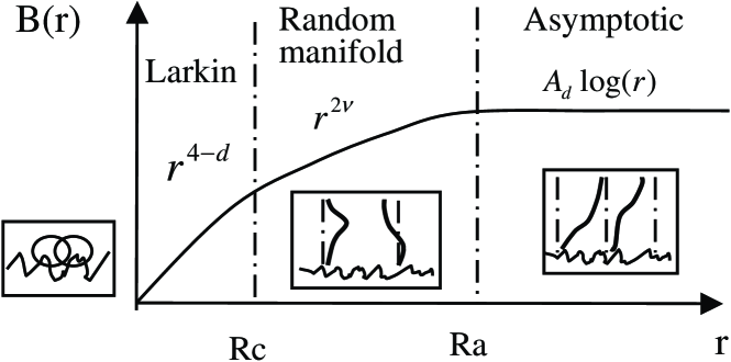
Figure 15: The relative displacement correlation function $B(r)$ as a function of distance. The lengthscales $R_{c}$ and $R_{a}$ define three regimes. Below $R_{c}$ one recovers the Larkin behavior. Between $R_{c}$ and $R_{a}$ the displacements still grow algebraically albeit with a modified exponent. Above $R_{a}$ the growth becomes logarithmic.

Three regime can be distinguished, separated by the characteristic lengthscales $R_{c}$ and $R_{a}$. Below $R_{c}$, one is in the Larkin regime, and the displacements grow as $r^{(4-d)/2}$. Then between $R_{c}$ and $R_{a}$ (i.e. when the displacements are between $\xi$ and $a$), each line wanders around its equilibrium position and the problem is very much like the one of a single line in a disordered environment, i.e. a random manifold problem. The growth of displacements is still algebraic, albeit with a different exponent $\nu$. Above $R_{a}$ however the displacements grow much more slowly and $B(r)=A_{d}\log(r)$. The physics is easy to understand: because of the periodic nature of the system, each line can take care of the disorder around its equilibrium position. There is thus no interest for one line to make displacements much larger than the lattice spacing to pass through a particularly favorable region of disorder (this would be the case for a single line). For many lines it is better to let the line closeby take care of this region. This ensures that the total energy of the whole system is the lowest. As a results the displacements do not need to grow much above $a$. The variational method and RG techniques allow to compute the prefactor $A_{d}$ and to address the issue of the positional order. The positional correlation function is simply given by giamarchi_vortex_short ; giamarchi_vortex_long

$$C(r)\sim\left(\frac{1}{r}\right)^{\eta}$$ (28)

where $\eta$ is an exponent independent of the strength of disorder or temperature (for example $\eta_{\rm var}=1$ in $d=3$). The physics described above, and obtained from the variational ansatz is totally generic. The alternate RG approach in $4-\epsilon$ does indeed recover identical physics, as was shown first in the Larkin and asymptotic regimes giamarchi_vortex_short ; giamarchi_vortex_long and more recently for the full $B(r)$ emig_exponents_braggglass . The variational approach even gives quite accurate values of the exponents themselves as can be checked by comparing with the RG. The quite striking consequence is that far from having the positional order destroyed by the disorder in an exponential fashion, a quasi-long range order (algebraic decay of positional order) exists in the system. Algebraically divergent Bragg peaks still exist as shown on Fig. 16.

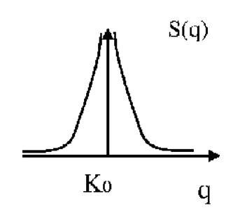
Figure 16: The disordered system still has quasi-long range positional order and algebraically divergent Bragg peaks. It is thus nearly as ordered as a perfect solid. Such a phase, which is a glass when one looks at its dynamics properties, and in addition possesses perfect topological order (no defects such as dislocations) is the Bragg glass phase giamarchi_vortex_long .

It is to be noted that this phase, which is thus practically as ordered as a perfect solid, is a glass when one looks at its dynamical properties. This is seen in the analysis by the presence of replica symmetry breaking in the variational approach or the existence of non-analyticities in the renormalization solution. From a physical point of view this means that the system has many metastable states separated from its ground state by divergent barriers. As a result it exhibits pinning and non-linear dynamics (creep motion), as we will discuss in more details in Section 5.

What about the argument that dislocations should always be generated at lengthscale $R_{a}$ ? In fact it was shown giamarchi_vortex_long that this argument which forgets the fact that the coupling of the displacements to the disorder is non linear is simply incorrect and that in fact in $d>2$ dislocations are not generated by disorder provided the disorder is moderate (i.e. $R_{a}$ large enough compared to $a$). This means that the results given above corresponds to the true thermodynamic ground state of the system. Thus there exists a thermodynamically stable glassy phase, the Bragg glass, with quasi long range order (algebraically divergent Bragg peaks), perfect topological order (absence of defects such as dislocations). This is a surprising result since one naively associate a glass with a very scrambled system. The Bragg glass shows that this is not the case and that one has to distinguish the positional properties from the energy landscape (or the dynamical ones).

The existence of this Bragg glass phase has of course many consequences for the vortex systems, consequences that we now investigate and compare with the available experimental data on vortices.

4.2 Positional order: Decorations and Neutrons

The first consequence is the existence of the perfect topological order and the algebraic Bragg peaks.

On the theoretical side, after the initial proposal giamarchi_vortex_long the existence of algegraic bragg peaks and the absence of dislocations have been confirmed by further analytical results carpentier_bglass_layered ; kierfeld_bglass_layered ; fisher_bragg_proof and numerical simulations gingras_dislocations_numerics ; vanotterlo_bragg_numerics . On the experimental side, direct structural information has been obtained from both real space studies such as magnetic decoration, scanning tunneling microscopy, Lorentz microscopy and reciprocal space studies by neutron diffraction, summarized in Fig. 17. The upper two panels show a decoration micrograph of a fairly ordered lattice in NbSe2 with a few defects marchevsky_thesis and an STM micrograph hess_stm_vortex of the same material with no defects. The Lorentz micrograph in a thin film of Nb harada_lorentz_vortex produces a nearly amorphous vortex assembly while the neutron diffraction data on a single crystal sample of Nb ling_neutrons_bragg show Bragg peaks up to third order reflections, suggesting a very high degree of order. These results show that defect-free phases with Bragg reflections are experimentally observed, while highly defective or even amorphous or liquid like phases also exist. The task is to find which parts of the phase space are occupied by each and what controls the phase transformations among them.

The fourier transforms of the real space data grier_decoration_manips ; marchevsky_thesis ; kim_decorations_nbse show very large regions free of dislocations and yield Bragg peaks routinely, suggesting a much stronger solid like order than would be expected naively from a vortex glass model. The situation with neutron diffraction is similar as shown on Figure 17.

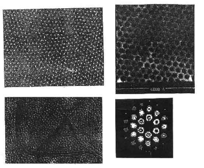
Figure 17: Vortex phase structure using various methods. The upper two panels show a decoration data on the leftmarchevsky_thesis and an STM data on the right in NbSe2hess_stm_vortex . The lower two panels show a Lorentz holography micrograph of a thin film Nbharada_lorentz_vortex and a neutron diffraction picture of a single crystal Nbling_neutrons_bragg

Recently neutron data have provided a direct evidence of the presence of the Bragg glass phase. Indeed the power-law Bragg peaks shown in Fig. 16 gives when convolved with the experimental resolution the result shown in Fig. 18. The width at half width of the observed peak is constant and determined by the experimental resolution, and the height is fixed by the position correlation length $R_{a}$. Thus if disorder (or magnetic field – see in the next section) is increased the Bragg glass predicts that observed neutron peaks should collapse without broadening. This behavior, has been quantitatively tested on the compound (K,Ba)BiO₃ klein_brglass_nature (see Fig. 18) which has the advantage of being totally isotropic and thus avoid all complications associated with anisotropy such as possible 2D-3D crossovers. Peaks are seen to collapse without any broadening thus providing a direct evidence of the Bragg glass phase and its algebraic positional order.

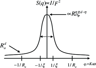
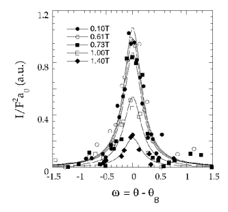
Figure 18: (left) Bragg glass predictions for the angular dependence of the neutron diffracted intensity when a finite experimental resolution is taken into account. The arrows indicate the values of $S(q)$ for $q=0$ and $1/R_{a}$ respectively. If the disorder increases (Ra decreases), the height of the peak decreases as $R_{a}^{\eta}$ but the peak does not broaden since the half width at half maximum is always given by the experimental resolution $1/\xi$ and not $1/R_{a}$. The height of the peaks gives a direct measure of the characteristic length $R_{a}$.(right) Angular dependence of neutron intensity diffracted by a (K,Ba)BiO₃ crystal klein_brglass_nature at the indicated applied fields. Those data show that the diffracted intensity (rocking curves) collapse without any broadening above $~{}0.7T$.

4.3 Unified phase diagram

Another striking consequences of the existence of the Bragg glass, is that it imposes a generic phase diagram for all type II superconductors giamarchi_vortex_long . Indeed the Bragg glass has no dislocations, thus if either thermal fluctuations or disorder are increased the Bragg glass should “melt” to a phase that contains defects . If thermal fluctuations increase this is the standard melting and leads to the liquid phase. Because the Bragg glass is nearly as ordered as a perfect solid one can expect it to melt though a first order phase transition. More importantly this “melting” of the Bragg glass can also occur because the disorder is increased in the system. For vortices increasing the field has a similar effect. Indeed the effective disorder in (9) is $V\rho_{0}$, thus increasing the average density makes the disorder term stronger compared to the elastic term (1). Indeed for moderate fields the change in elastic constants due to the field is quite small. Thus increasing the field is like increasing disorder. One should thus have a “melting” transition of the Bragg glass (induced by the disorder) as a function of the field. Close to $H_{c1}$ because the change of elastic constants is then drastic, one expects a similar transition. This leads to the universal phase diagram shown in Fig. 19.

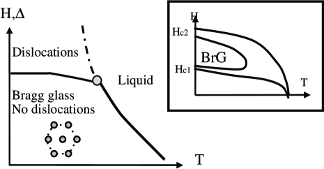
Figure 19: Universal phase diagram for type II superconductors. The Bragg glass “melts” due to thermal fluctuations of disorder induced fluctuations. This lead to transitions as a function of magnetic field. The left diagram is far from $H_{c1}$ (more adapted to High Tc) whereas the insert shown the full diagram. The melting towards the liquid is expected to be first order.

We first focus on the experimental results of the loss of Bragg glass order in the cuprate systems. A remarkable experimental determination of the phase diagram of BSCCO is shown in Fig. 20.

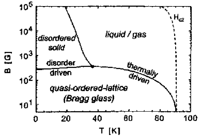
Figure 20: Experimental phase diagram for the cuprate system BSCCO zeldov_diagphas_bisco ; khaykovich_diagphas_bisco . At the thermally induced melting transition one sees thermodynamic anomalies as in Fig. 8. The disorder-driven transition is accompanied by the second peak or peak effect, shown later in Fig. 26.

Three phases are clearly identified in it : a quasi-ordered Bragg glass phase which “melts” by thermal fluctuations into a liquid and also “amorphizes” or “melts” by quenched disorder into a disordered solid. First we focus on structural evidence of the two phase transitions from neutron diffraction cubbit_neutrons_bscco . In the Bragg glass phase one clearly observes the resolution limited Bragg peaks. Upon increasing temperature across the thermally driven transition the Bragg peaks lose intensity and become unobservable in the putative liquid phase. A similar loss of Bragg peak intensity is observed when the magnetic field is increased at fixed $T$ across the Bragg glass to the disordered or vortex glass phase. Fig. 21 and Fig. 22 show the results of neutron diffraction of BSCCO as the two phase boundaries are crossed, one from the ordered Bragg glass to the liquid and the other from Bragg glass to the disordered solid phase cubbit_neutrons_bscco .

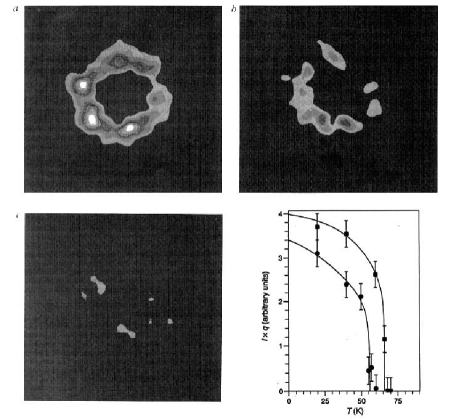
Figure 21: Evolution of the neutron bragg peaks in the ordered phase (upper left panel) with increasing temperature. The lower right panel shows the loss of Bragg intensity with increasing T

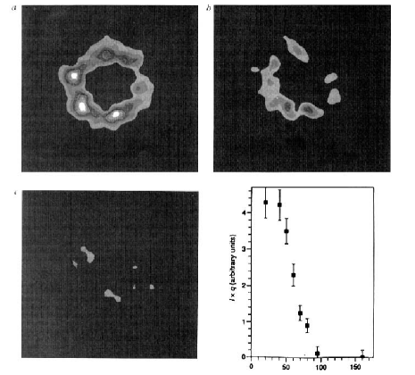
Figure 22: Loss of Bragg intensity upon increasing the magnetic field at a fixed temperature

In both cases the Bragg reflections lose intensity and disappear at the phase boundary, in a way similar to the one discussed in Fig. 18. Due to limited neutron intensity, detailed studies of the disordered phase has not been performed in the cuprates. But recent neutron diffraction studies of low Tc system Nb gammel_neutrons_Nb ; ling_neutrons_bragg with a short penetration depth have directly shown a transformation of bragg peaks to a ring of scattering, implying liquid like (amorphous) order in the disordered phase. The experimental phase behavior is thus entirely compatible with theoretical expectations in Fig. 19. The comparison with the theoretical phase diagram identifies the quasi-ordered solid phase with the Bragg glass phase. The phase with dislocations is expected to correspond to the disordered solid phase. For BSCCO the position of the field melting line has been computed by Lindemann argument or similar cage arguments ertas_diagphas_bisco ; giamarchi_diagphas_prb ; kierfeld_diagphas_bisco ; koshelev_diagphas_bisco and the value of the “melting” field is in good agreement with the observed experimental value. The distinction between the disordered solid phase and the liquid phase remains an experimentally open question for different systems with different types of disorder. For the very anisotropic BSCCO system there is also the question of the existence of additional phases. Structural results of the same kind are not available for the other common cuprate system, namely YBCO. However, thermodynamic data on the magnetization jump and entropy jump were measured. A composite of the data is shown in Fig. 23 (see also bouquet_melting_ybco ) which demonstrates close agreement within the Clapeyron equation confirming the first order nature of the thermally driven melting transition.

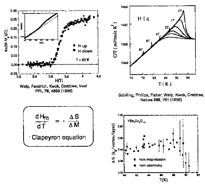
Figure 23: Experimental data welp_magnetization_jump ; schilling_heat_vortex showing thermodynamic measurements from magnetization and calorimetry of the first order transition in YBCO

4.4 Second peak and peak effect

Now we focus on the disorder driven phase transition shown above. The magnetization hysteresis loop across this transition manifests a typical second peak effect, often called the fishtail effect due to its shape, as shown in Fig. 24 for BSCCO khaykovich_diagphas_bisco .

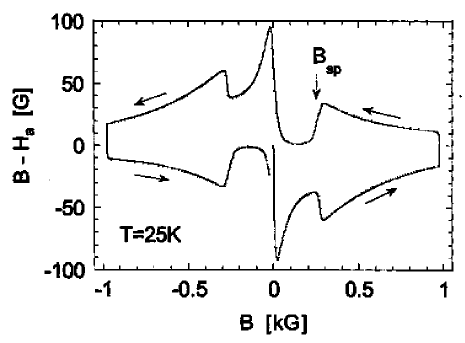
Figure 24: Typical second magnetization peak data from the magnetic hysteresis loop in BSCCOkhaykovich_diagphas_bisco , the sudden enhancement of the diamagnetic signal at $B_{sp}$ marks the enhancement of critical current across the Bragg glass to vortex glass phase transition.

The sharp jump is magnetization at $B_{sp}$ marks a sudden increase in the irreversibility, i.e., a jump in critical current $J_{c}$. In a naive view of the Larkin scenario, this marks a sudden decrease in the correlation volume, i.e., a sharp loss of order, consistent with the neutron diffraction data shown above. Similar results were obtained for YBCO also, yielding a qualitatively similar phase diagram deligiannis_diagphas_ybco ; nishizaki_diagphas_ybco ; kokkaliaris_diagphas_ybco .

Peak effects are ubiquitous in low Tc systems and have been known for nearly four decades and provided the primary motivation for the Larkin-Ovchinnikov scenario of collective pinning. In these systems the peak effect wordenweber_kes_peak usually occurs very close to the normal phase boundary, unlike in the cuprate systems where the fishtail anomaly occurs very far from it. Recent resurgence of activity on the peak effect phenomenon in low Tc systems also provide a phase diagram of ordered and disordered vortex phases not dissimilar to the cuprates. Due to the smallness of the thermal fluctuation effects, however, the peak effect transition often occurs in close proximity to the melting transition, or even coincident with it. Separating the two effects remains a matter of considerable controversy in the low Tc systems. In the popular low Tc system NbSe2 the peak effect phenomenon has been studied extensively in recent years bhattacharya_peak_prl . Fig. 25 shows a typical set of data for the resistive detection of the peak effect where a rapid drop in the resistance at the peak effect boundary marks a sudden increase in the critical current analogous to the magnetization jump shown above.

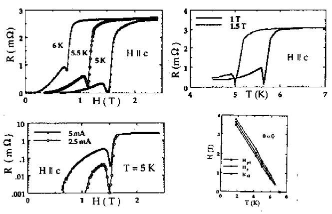
Figure 25: Typical observation of peak effect in transport higgins_second_peak . The upper two panels show the transition in isothermal and isofield measurements. The lower left panel shows the independence of the locus on driving current suggesting a thermodynamic origin of the anomaly. The right panel shows the locus of the peak region bounded by the onset at $H_{pl}$ and the peak at $H_{p}$. The close proximity to the upper critical field is typical of low $T_{c}$ materials..

Direct structural evidence also clearly shows the amorphization of the Bragg glass phase with six fold symmetric Bragg spots to a ring of scattering at the peak in the elemental system Nb ling_neutrons_bragg . In NbSe2 the same peak effect is accompanied by a sharp change in the line shape as seen in the asymmetry parameter rao_musr_peak . These results are shown in Fig. 26.

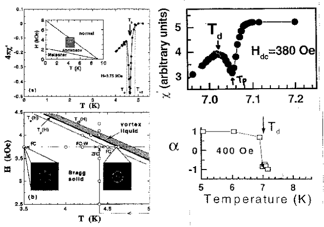
Figure 26: Experimental data on Nbling_neutrons_bragg on the left and NbSe2 rao_musr_peak on the right. The upper panel shows the peak effect from ac susceptibity for both. The lower left panel shows the structure from neutron diffraction in Nb showing the Bragg spots disappear into a ring of scattering. Muon spin relaxation data in NbSe2 on the right shows a sudden drop in the skewness parameter at the peak effect that marks the first order structural disordering of the lattice.

Of special importance is the clear experimental observation of a reentrant phase behavior for the NbSe2 system ghosh_reentrant_peak ; banerjee_reentrant_peak . From the Meissner phase an increase in field shows two anomalies, first from a disordered phase into an ordered phase and then a reentry into a disordered phase just below the upper critical field. Especially significant is the pronounced shift in the order-disorder phase boundary with varying quenched disorder (addition of magnetic dopants). Figure 27 shows the progressive shrinkage of the Bragg glass phase from both high field side as well as from the low field side as disorder is increased from sample A through sample C.

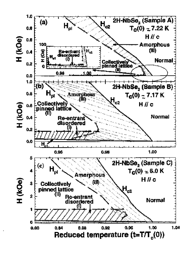
Figure 27: Evolution of the phase diagram banerjee_reentrant_peak with increased disorder from sample A to C. As disorder increases, the collectively pinned lattice, i.e., the Bragg glass phase, shrinks from both above and below.

These results are in excellent agreement with the theoretical discussions above. Direct structural evidence of amorphization in this system was obtained through muon spin relaxation experiments rao_musr_peak that are entirely analogous to the results aegerter_YBCO_musr in the cuprate systems.

Several questions remain open for the peak effect from the phase behavior point of view. In addition to the second magnetization peaks, a peak effect is often observed in YBCO very close to or even coincident with the melting transition ishida_peak_melting . This suggests that the disordered solid phase may protrude as a sliver all around the Bragg glass phase menon_phasediag_univ or that there are two types of peak effects, one associated with disorder induced melting and the other with the thermally induced melting transition. In what follows, we indeed show that the melting of the Bragg glass provides a natural explanation for the peak effect.

How the melting of the Bragg glass signals itself ? To understand it let us look at the $V-I$ characteristics, shown on Fig. 28.

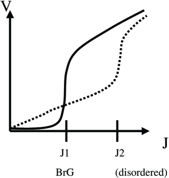
Figure 28: The $V-I$ characteristics for the Bragg glass (full line) and the high field phase or the liquid (dashed line) giamarchi_diagphas_prb .

The Bragg glass is collectively pinned so it has a small critical current $J_{1}$ but very high barriers leading to practically no motion (hence no $V$) in the pinned phase (below $J_{1}$). On the other hand in the high field phase (with dislocations) or the liquid it is more easy to pin small parts leading to higher critical currents, but the pinning is not collective hence a much more linear response below $J_{2}$. The $V-I$ characteristics thus cross at the melting of the Bragg glass giamarchi_diagphas_prb . This crossing leads for an apparent increase of the critical current close to the melting and thus to a peak effect in the transport measurements or to a second peak in the magnetization measurements.

Recent simulations and reexamination of older experimental data vanotterloo_IV_peakeffect ; higgins_second_peak are in excellent agreement with this $I-V$ crossing scenario at the peak effect near melting or the second magnetization peak.

5 Dynamics of vortices

The competition between disorder and elasticity manifests also in the dynamics of such systems, and if any in a more dramatic manner. When looking at the dynamics, many questions arise. Some of them can be easily asked (but not easily answered) when looking at the $V-I$ characteristics shown in Fig. 29.

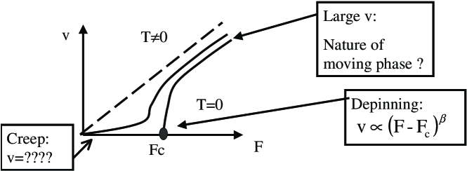
Figure 29: The $V-I$ characteristics for a vortex system. This is in fact the velocity of the system $v$, in response to an external force $F$.

The simplest question is prompted by the $T=0$ behavior. Since the system is pinned the velocity is zero below a certain critical force $F_{c}$. For $F>F_{c}$ the system moves. What is $F_{c}$ ? We saw that the scaling theory of Larkin and Ovchinikov relates it directly to the static characteristic length $R_{c}$. Can one extract this critical force directly from the solution of the equation of motion of the vortex lines

$$\eta\frac{du_{i}(t)}{dt}=-\frac{\delta H}{\delta u_{i}}+F+\zeta_{i}(t)$$ (29)

This equation is written for overdamped dynamics, but can include inertia as well. $\eta$ is the friction coefficient taking into account the dissipation in the cores, $F$ the externally applied force, and $\zeta$ a thermal noise. Can one obtain from this equation the velocity above $F_{c}$ ? The $v-F$ curve at $T=0$ is reminiscent of the one of an order parameter in a second order phase transition. Here the system is out of equilibrium so no direct analogy is possible but this suggests that one could expect $v\sim(F-F_{c})^{\beta}$ with a dynamical critical exponent $\beta$. We will not investigate these questions here, because of lack of space and refer the reader to the above mentioned reviews and to chauve_creep_long for an up to date discussion of this issue and additional references.

The second question comes from the $T\neq 0$ curve. Well below threshold $F\ll F_{c}$ the system is still expected to move through thermal activation. What is the nature of this motion and what is the velocity ? If the system has a glassy nature one expects it to manifest strongly in this regime since thermal activation will have to overcome barriers between various states. We address this question in Section 5.1.

Finally, there are many questions beyond the simple knowledge of the average velocity. One of the most interesting is the nature of the moving phase. If one is in the moving frame where the system looks motionless, how much this moving system resembles or not the static one. This concerns both the positional order properties and the fluctuations in velocity such as the ones measured in noise experiments. This is discussed in Section 5.2.

5.1 Creep

Let us first examine the response of the vortex system to a very small external force. For usual systems we expect the response to be linear (leading to a finite resistivity for the system). Indeed earlier theories of such a motion found a linear response. The idea is to consider that a blob of pinned material has to move in an energy landscape with barriers $\Delta$ as shown in Fig. 30.

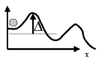
Figure 30: In the Thermally Assisted Flux Flow (TAFF) anderson_kim a region of pinned material is considered as a particle moving in an energy landscape with barriers. This leads to an exponentionally small but linear response.

The external force $F$ tilts the energy landscape making forward motion possible. The barriers are overcome by thermal activation (hence the name: Thermally Assisted Flux Flow) with an Arrhenius law. If the minima are separated by a distance $a$ the velocity is

$$v\propto e^{-\beta(\Delta-Fa/2)}-e^{-\beta(\Delta+Fa/2)}\simeq e^{-\beta\Delta}F$$ (30)

The response is thus linear, but exponentially small. One thus recovers that pinning drastically improves the transport qualities of superconductors. For old superconductors $\beta$ was small enough so that this formula was not seriously challenged. However with high $T_{c}$ one could reach values of $\beta$ where it was clear that the TAFF formula was grossly overestimating the motion of vortex lines.

The reasons is easy to understand if one remembers that the static system is in a vitreous state. In such states a “typical” barrier $\Delta$ does not exist, but barriers are expected to diverge as one gets closer to the ground state of the system. The TAFF formula is thus valid in system where the glassy aspect is killed. This is the case in the liquid where various parts of the system are pinned individually. When the glassy nature of the system persists up to arbitrarily large lengthscales the theory should be accommodated to take into account the divergent barriers fisher_vortexglass_short ; fisher_vortexglass_long . This can be done quantitatively within the framework of the elastic description. In fact such a theory was developed before for interfaces nattermann_rfield_rbond ; ioffe_creep and then adapted for periodic systems such as the vortex lattice feigelman_collective ; nattermann_pinning . The basic idea is beautifully simple. It rests on two quite strong but reasonable assumptions : (i) the motion is so slow that one can consider at each stage the lattice as motionless and use the static description; (ii) the scaling for barriers which is quite difficult to determine is the same than the scaling of the minimum of energy (metastable states) that can be extracted again from the static calculation. If the displacements scale as $u\sim L^{\nu}$ then the energy of the metastable states (see (1)) scale as

$$E\sim L^{d-2+2\nu}$$ (31)

on the other hand the energy gained from the external force over a motion on a distance $u$ is

$$E_{F}=\int d^{d}xFu(x)\sim FL^{d+\nu}$$ (32)

Thus in order to make the motion to the next metastable state one needs to move a piece of the pinned system of size

$$L_{\rm min}\sim\left(\frac{1}{F}\right)^{\frac{1}{2-\nu}}$$ (33)

The size of the minimal nucleus able to move thus grows as the force decrease. Since the barriers to overcome grow with the size of the object the minimum barrier to overcome (assuming that the scaling of the barriers is also given by (31))

$$\Delta(F)\sim\left(\frac{1}{F}\right)^{\frac{d-2+2\nu}{2-\nu}}$$ (34)

leading to a velocity

$$v\propto e^{-\beta\left(\frac{1}{F}\right)^{\frac{d-2+2\nu}{2-\nu}}}$$ (35)

This is a remarkable equation. It relates a dynamical property to static exponents, and shows clearly the glassy nature of the system. The corresponding motion has been called creep since it is a sub-linear response. Of course the derivation given here is phenomenological, but it was recently possible to directly derive the creep formula from the equation of motion of the system chauve_creep_short ; chauve_creep_long . This proved the two underlying assumptions behind the creep formula and in particular that the scaling of the barriers and metastable states is similar. More importantly this derivation shows that although the formula for the velocity given by the phenomenological derivation is correct, the actual motion is more complicated than the naive phenomenological picture would suggest. Indeed the phenomenological image is that a nucleus of size $L_{\rm min}$ moves through thermal activation over a length $L_{\rm min}^{\nu}$, and then the process starts again in another part of the system. In the full solution, one finds that the motion of this small nucleus triggers an avalanche in the system over a much larger lengthscale chauve_creep_long . Checking for this two scales process in simulations or actual experiments if of course a very challenging problem.

The creep formula is quite general and will hold for interfaces as well as periodic systems. For periodic systems, dislocations might kill the collective behavior by providing an upper cutoff to the size of the system that behaves collectively (as if the system was torn into pieces). In the Bragg glass the situation is clear. Since there are no dislocations the creep behavior persists to arbitrarily large lengthscales. Since $\nu=0$ in the Bragg glass the creep exponent in (35) is $\mu=0.5$ nattermann_pinning ; giamarchi_vortex_long . What becomes of the creep when dislocations are present is still an open kierfeld_plastic_creep and very challenging question. What is sure is that one can expect a weakening of the growth of the barriers or even their saturation, when going from the Bragg glass phase to the “melted” phase giamarchi_diagphas_prb . This is at the root of the crossing of the $I-V$ shown in Fig. 28. Experimental verification of the creep effects postulated above have proved difficult due to the functional form of (35) where the power law appears in the exponentiated factor and requires data spanning many decades in the drive to determine the exponents with adequate precision. Transport experiments fuchs_creep_bglass as well as magnetic relaxation experiments vanderbeek_relaxation_exponents have reported creep exponents compatible with the Bragg glass prediction, as well as weakening of the barrier growth when going to the disordered phase. But this is clearly a very challenging and difficult issue that would need more investigations.

5.2 Dynamical phase diagram

Let us now turn to the problem of the nature of the moving phase.

This problem was directly prompted by experimental observations. Indeed early measurements of the dynamics showed dramatic effects near the peak effect (see below), led to the construction of an experimental dynamical ”phase diagram” bhattacharya_peak_prl for the moving phases shown in Fig. 31.

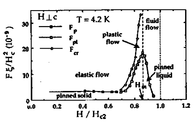
Figure 31: A typical dynamic phase diagram in NbSe2. Below the transition region a direct transition into a moving ordered phase is seen while in the peak regime a pronounced intermediate plastic flow regime is seen. At large drives above $F_{cr}$, the moving ordered phase is established. In the equilibrium pinned liquid phase, the crossover current is immeasurably large.

In addition dramatic evidence of the evolution of vortex correlations with driving force was obtained many years ago by neutron diffraction studies thorel_neutrons_vortex . The Bragg peak in the pinned phase broadened significantly at the onset of motion showing a loss of order (or appearance of defects) and a subsequent healing of the Bragg peak at large drives showing a reentry into an ordered moving phase. It was thus necessary to understand the nature of the “phases” once the lattice was set into motion.

One regime in which one could think to tackle this problem is when the lattice is moving at large velocities. Indeed in that case it is possible to make a large velocity expansion. Such expansion was performed with success to compute the corrections to the velocity due to pinning larkin_largev ; schmidt_hauger , and get an estimate of the critical current. An important step was to use the large $v$ method to compute the displacements koshelev_dynamics . It was found that due to the motion the system averages over the disorder. As a result the system do not feel the disorder any more above a certain lengthscale and recrystalizes. The memory of the disorder would simply be kept in a shift of the effective temperature seen by this perfect crystal. This picture was consistent with what was shown to be true for interfaces, even close to threshold nattermann_stepanow_depinning (as shown on Fig. 32) and thus provided a nice explanation for the recrystallization observed at sufficiently large velocities. Perturbation approach along those lines has been extended in scheidl_perturbative_phasediag .

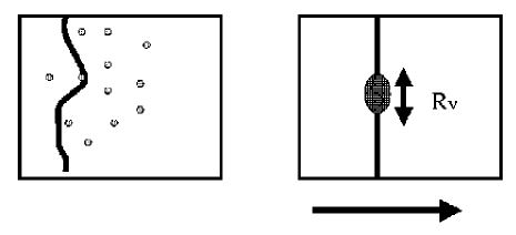
Figure 32: When an interface is in motion, it averages over the disorder. As a result the interface does not feel the disorder above a certain lengthscale $R_{v}$ and becomes flat again.

However the peculiarities of the periodic structure manifests themselves again, and they does not follow this simple scenario, the way that the interfaces would. The crucial ingredient present in periodic system is the existence of a periodicity transverse to the direction of motion. Because of this, the transverse components of the displacements still feel a disorder that is non averaged by the motion. As a result the large-$v$ expansion always breaks down, even at large velocities and cannot be used to determine the nature of the moving phases. To describe such moving phase the most important components are the components transverse to the direction of motion (this is schematized in Fig. 33).

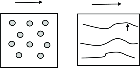
Figure 33: When in motion a periodic structure averages over the Fourier components of disorder along the direction of motion whereas the component perpendicular to motion remains unaffected. As a result the components of the displacements transverse to the direction of motion are the essential ingredients to describe a moving system.

The motion of these components can be described by a quite generic equation of motion, as explained in giamarchi_moving_prl ; ledoussal_mglass_long . The transverse components still experience a static disorder, and as a result the system in motion remains a glass (moving glass).

In the moving glass the motion of the particles occurs through elastic channels as shown in Fig. 34.

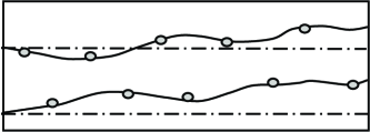
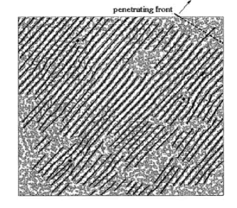
Figure 34: In a moving glass the motion occurs through elastic channels. The channels themselves are rough and meander arbitrarily far from a straight line, but all particles follows on these channels like cars on a highway. These channels have been observed in decoration experiments, as shown on the left marchevsky_decoration_channels

The channels are the best compromise between the elastic forces and the static disorder still experienced by the moving system. Like lines submitted to a static disorder the channels themselves are rough and can meander arbitrarily far from a straight line (displacements grow unboundedly). However although the channels themselves are rough, the particles of the system are bound to follow these channels and thus follow exactly the same trajectory when in motion. Needless to say the moving system (moving glass) is thus very different than a simple solid with a modified temperature where the particles would just follow straight line trajectories (with a finite thermal broadening).

When does this picture breaks down ? Clearly this should be the result of defects appearing in the structure. For example close to depinning, it was shown experimentally bhattacharya_peak_prl (see Fig. 31) that some of the regions of the system can remain pinned while other parts of the system flow, leading to a plastic flow with many defects. One thus need to check again for the stability of the moving structure to defects. Fortunately the very existence of channels provide a very natural framework to study the effect of such defects: they will lead quite naturally to a coupling and a decoupling of the channels giamarchi_moving_prl ; balents_mglass_long ; ledoussal_mglass_long ; scheidl_perturbative_phasediag .

The various phases that naturally emerges in $d=3$ are thus the ones shown in Fig. 35 (a similar study can be done for $d=2$).

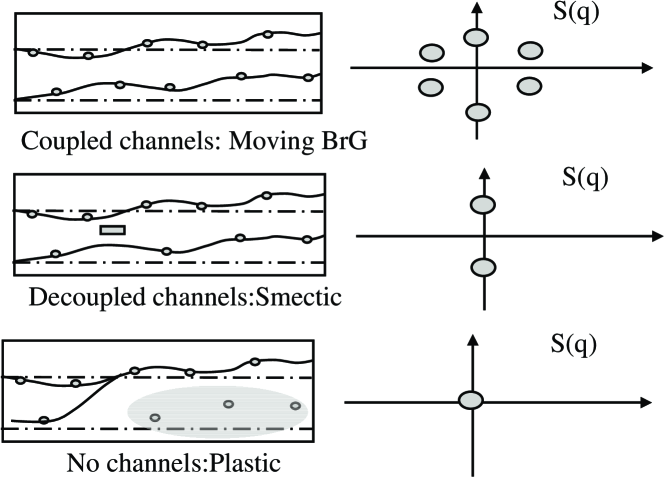
Figure 35: The various dynamical phases of a moving periodic system.

At large velocity the channels are coupled and the system possesses a perfect topological order (no defects). The moving glass system is thus a moving Bragg glass. The structure factor has six Bragg peaks (with algebraic powerlaw divergence) showing that the system has quasi-long range positional order. If the velocity is lowered a Lindemann analysis shows that defects that appear first tend to decouple the channels. This means that positional order along the direction of motion is lost, but since the channel structure still exist a smectic order is preserved (channels become then the elementary objects). As a result the structure factor now has only two peaks. This phase is thus a moving smectic (or a moving transverse glass, as first found in moon_moving_numerics ). It is important to note that in these two phases the channel structure is preserved and described by the moving glass equation. Both these phases are thus a moving glass. A quite different situation can occur if the velocity is lowered further. In that case the channel structure can be destroyed altogether, leading to a plastic phase. Note that depending on the amount of disorder in the system this may or may not occur, and in $d=3$ a purely elastic depinning could be possible in principle (in $d=2$ the depinning is always plastic). These various phases lead to the dynamics phase diagram shown in Fig. 36.

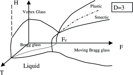
Figure 36: The dynamical phase diagram ledoussal_mglass_long as a function of the temperature $T$, the magnetic field (far from $H_{c1}$) and the applied force $F$. Both the Bragg glass and the Moving Bragg glass have perfect topological order.

These various phases as well as the dynamical phase diagram have been confirmed in numerous simulations (see e.g. moon_moving_numerics ; olson_mglass_phasediag ; kolton_mglass_phases ; fangohr_mglass_phasediag ).

Let us now turn to the experimental analysis of the dynamics. Early experiments on the dynamics of the vortex phases near the peak effect bhattacharya_peak_prl showed that not only does the critical current rise sharply at the transition, but the $I-V$ curves also change in character. This is shown schematically in fig. 37.

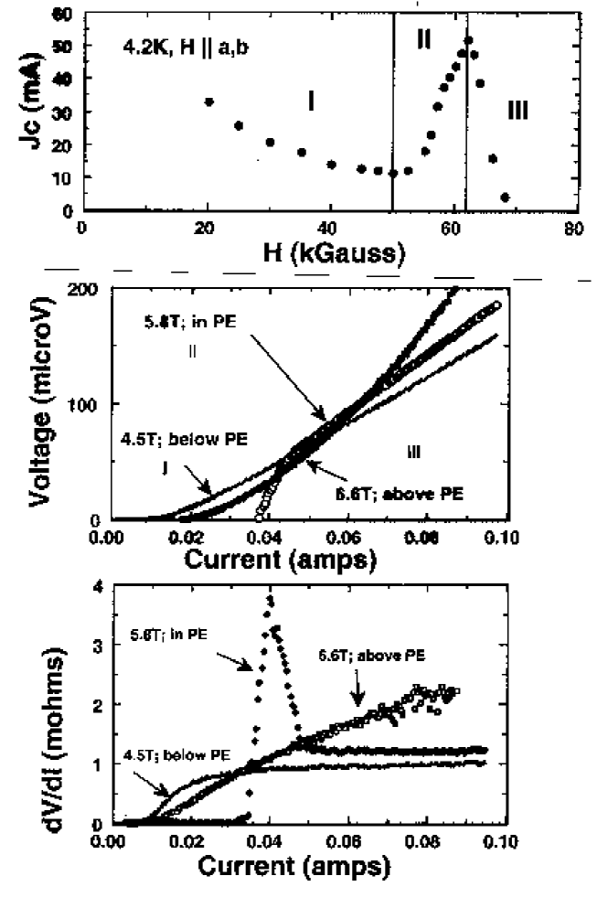
Figure 37: Summary of the variation in the I-V characteristic across the peak effect, i..e., ordered to disordered phase transition bhattacharya_peak_prl . The upper panel shows the peak effect transition and marks the three regimes of flow. The middle and lower panels show the I-V curves and the dV/dI-I curves for the three regimes.

The top panel shows the peak effect at a fixed $T$ and varying $H$. Three distinct types of I-V curves are observed in the regions marked I, II and III, shown in the middle panel. In the peak region the curves show opposite curvature to that in the other regions, the voltage grows convex upwards. The lower panel illustrates this behavior through the differential resistance Rd ($=dV/dI$)for each region. In the peak region it shows a pronounced maximum above which it rapidly decreases to a terminal asymptotic value of the Bardeen-Stephen flux flow resistance above a crossover current. A comparison with simulations faleski_marchetti_dynamics shown in Fig. 38 suggests that the peak signifies a plastic flow region where the vortex matter moves incoherently and a coherent flow is recovered at high drives.

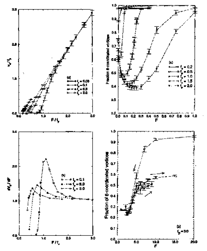
Figure 38: Simulation data faleski_marchetti_dynamics of the force-velocity curves together with the variation of defect density with driving force. Compare the simulation data with the experimental data for plastic flow.

This behavior contrasts with that in region I below the peak effect where the pinned vortex matter is in the Bragg glass phase. In this case the flux flow resistance is approached monotonically without a measurable signature of plastic flow. The plastic flow regime is also accompanied with pronounced fingerprint effect: a repeatable set of features in Rd as the current is ramped up and down, signifying a repeatable sequence of chunks of pinned vortex assembly depinning and joining the main flow. This clearly establishes the defective nature of the moving vortex matter in this regime. The contrast with this behavior in region I is thought to represent a depinning of the Bragg glass phase directly into a moving Bragg glass phase.

A striking result is seen in the behavior of the flux flow noise marley_broadband_noise , summarized in Fig. 39.

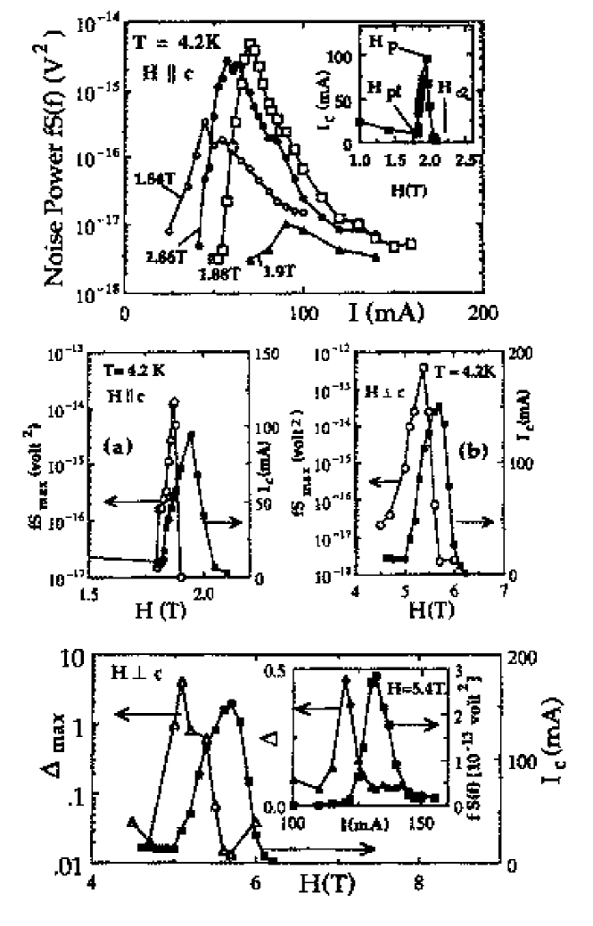
Figure 39: Noise characteristics in the plastic flow regime marley_broadband_noise . The upper panel shows the current dependence of the noise which turns on at the critical current and depletes at large current when a moving ordered phase is recovered. The middle panels show the field dependence of the noise; it is restricted only to the peak regime. The lowest panel show a measure of the non-gaussianity of the noise which is maximum (i.e.,few noise sources) at the onset of motion supporting the moving “chunk” scenario in the plastic flow regime.

The noise is larger in the peak regime by orders of magnitude (seen in the lower panel) and is restricted to current values between the depinning current and the crossover current (shown in the upper panel). The noise is, therefore, associated with an incoherent flow of a defective moving phase and a coexistence of moving and pinned vortex phases as was seen in detailed studies merithew_vortex_noise ; rabin_vortex_noise . The qualitative behavior observed in the experiment is consistent with many simulations of the flux flow noise characteristics. However, recent work suggests that an edge contamination mechanism in the peak regime is responsible for triggering much of the defective plastic flow in the bulk and is a subject under active investigation paltiel_edge_cont ; marchevsky_peakeffect_nbse . There have also been reports of narrow band noise togawa_mglass_noise , i.e., noise peaks at the so-called washboard frequency. The observation of such noise would be compatible with the moving Bragg glass phase.

More experimental evidence in favor of the moving glass is also found in recent decoration and STM studies of the moving vortex assembly pardo_decoration_mglass ; marchevsky_decoration_channels ; troyanovski_stm_flow .

5.3 Metastability and history dependence

A current focus on experimental vortex phase studies is a renewed interest in history effects that have long been known to occur in vortex matter. In order to understand the equilibrium phase behavior of the system, we need to ascertain that we have indeed reached equilibrium in an experiment. However, most experiments in low Tc systems and at low temperatures in high Tc systems as well, show a pronounced dependence of the vortex correlations on the thermomagnetic history of the system. A striking example is shown in Fig. 40 where the magnetic response banerjee_history_dep ; ravikumar_history_dep , and transport critical current henderson_history_dep are measured for field cooled (FC) and zero field cooled(ZFC) cases.

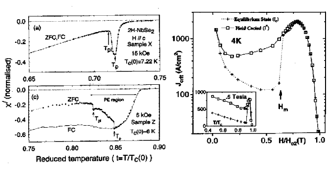
Figure 40: History dependence of the critical current seen with magnetic susceptibility(left) banerjee_history_dep , and transport(right) henderson_history_dep . For a very clean sample on the top panel on the left, no history effect is seen unlike the bottom panel for a dirty sample. The peak of the peak effect marks the onset of an equilibrium disordered phase.

In the latter case one sees a pronounced peak effect but not in the former. In other words, the FC state yields a highly disordered vortex glass phase and the latter yields an ordered Bragg glass phase. The question then is : which is the stable and equilibrium state of the system and how does one find it ? A similar question arose in the interpretation of neutron experiments yaron_neutrons_vortex where it was suggested giamarchi_vortex_comment that the observed broadening of the lines that disappeared after a cycling above the critical current, was due to the presence of out of equilibrium dislocations (on the top of the equilibrium Bragg glass phase).

One possible resolution of the problem comes from a ”shaking experiment” where the FC state is subjected to a large oscillatory magnetic field and the system evolves to the ZFC state banerjee_shake_switch . Once in the ZFC ordered state, below the peak effect, the system cannot be brought to the FC disordered state regardless of any external perturbation. It is thus reasonable to conclude that the ordered (Bragg glass) state is the equilibrium state below the peak effect. The FC disordered (vortex glass) phase is simply supercooled from the liquid phase above. When pinning sets in, the system fails to explore the phase space due to the pinning barrier and stays frozen into glassy, disordered phase. Shaking with an ac field then provides an annealing mechanism to bring the system in the true ground state which is the Bragg glass. On the other hand, shaking fails to produce an ordered state above the peak and thus the disordered phase is indeed the ground state there. Curiously then the ZFC state is formed by vortices entering the system at high velocity, thereby ignoring pinning and forming a moving Bragg glass phase from which the pinned Bragg glass phase evolves easily. Recent aging experiments portier_age_vortex have provided compelling evidence in support of these conclusions. Further evidence of a thermodynamic nature of the transition is obtained also from magnetization anomalies from annealed vortex states ravikumar_stable_phases .

5.4 Edge effects

Yet another phenomenon has begun to be explored in experimental studies paltiel_edge_cont ; marchevsky_peakeffect_nbse . This relates to the observation that edges of a sample provide nucleation centers for the disordered phase. The net results are (1) the order-disorder phase transition becomes spatially non-uniform and leads to phase coexistence that marks the width of the peak effect region and (2) an external driving current flows non-uniformly in the system. The contamination of the ordered phase by the disordered phase from the edge and the subsequent annealing back to the ordered phase at larger drives occur in a non-uniform manner leading to a variety of unusual time and frequency dependent phenomena observed earlier. Differentiating the effects of these processes from the bulk response of the system, usually assumed in interpreting data and in simulations, remains a subject of current study.

5.5 Transverse critical force

One of the unexpected consequences of the presence of channels in the moving glass phase, is the existence of transverse pinning giamarchi_moving_prl . Let us examine what would happen if one tried to push the moving system sideways by applying a force $F_{y}$ in a direction perpendicular to motion. This is depicted in Fig. 41

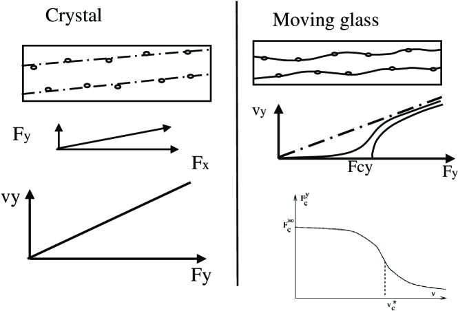
Figure 41: Response of the system to a force $F_{y}$ transverse to the direction of motion. Although a crystal would respond linearly, the moving glass remains pinned in the transverse direction although the particles are moving along the direction $x$ giamarchi_moving_prl ; ledoussal_mglass_long .

The naive answer would be that the system is submitted to a total force $F=F_{x}+F_{y}$ and because the modulus of this force is larger than the threshold ($F_{x}>F_{c}$ since the system is already sliding), the system will slide along the total force. This means that there is a linear response $v_{y}$ to the applied transverse force $F_{y}$. This is what would occur if the moving system was a crystal. However in the moving glass although the particles themselves move along the channels, the channels are submitted to a static disorder and thus pinned. It means that if one applies a transverse force, the channels will have to pass barriers before they can move. As a results the system is transversally pinned even though it is moving along the $x$ direction. The existence of this transverse critical force is a hallmark of the moving glass. It is a fraction of the longitudinal transverse force and decreases as the longitudinal velocity increases as shown on Fig. 41. The existence of such transverse force has been confirmed in many simulations (see e.g. moon_moving_numerics ; olson_mglass_transverse ; fangohr_mglass_transverse ). Its experimental observation for vortex systems is still an experimental challenge.

6 Conclusions and perspectives

It is thus clear from the body of work presented in these notes that the field of vortex matter has considerably matured in the last ten years or so. Many important physical phenomena have been unravelled, and a coherent picture starts to emerge. As far as the statics of the problem is concerned we start now to have a good handle of the problem. The Bragg glass description has allowed to build a coherent picture both of the phase diagram and of most of the previously poorly understood striking phenomena such as imaging, neutrons and peak effect or more generally transport phenomena. Important issues such as the contamination by the edge and the necessity to untangle these effects to get the true thermodynamics properties of the system are now understood, allowing to get reliable data. Although, understanding the dynamics is clearly much more complicated both theoretically and experimentally, here also many progress have been made. The vortex matter has allowed to introduce and check many crucial concepts such as the one of creep motion. For the dynamics also it is now understood that periodicity is crucial and that strong effects of disorder can persist even when a lattice is fast moving.

Of course the progress realized make only more apparent the many exciting issues not yet understood and that are waiting to be solved. For the statics the nature of the high field phase above the melting field of the Bragg glass is still to be understood. Is this phase a distinct thermodynamic phase from the liquid ? is it a true glass in the dynamical sense ? Many difficult questions that will need the understanding of a system in which disorder and defects (dislocations, etc.) play a crucial role. Similar question occur for the dynamics whenever a plastic phase occurs. There is thus no doubt that understanding the role of defects and disorder is now one of the major challenge of the field. The glassy nature of the various phases also certainly needs more detailed investigations, in particular the “goodies” such as aging that have been explored in details for systems such as spin glasses would certainly prove useful to investigate. Finally, both theorists and experimentalists have mostly focussed for the moment on the steady state dynamics. Clearly the issue of noise, out of equilibrium dynamics, and history dependence are challenging and crucial problems.

In addition, the material covered in these notes is only a part of the many interesting phenomena related to the physics of vortex lattices, and more generally disordered elastic systems. Because of space limitation, it would be impossible to cover here all these interesting aspects but we would like to at least mention few of them.

In addition to point like impurities there is much interest, both theoretical and practical, to introduce artificial disorder. The most popular is the one produced by heavy ion irradiation konczykowski_columnar_first ; civale_columnar_prl ; vanderbeek_columnar_long , leading to the so called columnar defects and to the Bose Glass phase nelson_columnar_long . Other types of disorder such as splay hwa_splay_prl or regular pinning arrays have also been explored. We refer the reader to the above mentioned reviews for more details on these issues.

Quite interestingly, the description of the vortices in term of elastic objects allows to make contact with a large body of other physical systems who share in fact the same effective physics. This ranges from classical systems such as magnetic domain walls, wetting contact lines, colloids, magnetic bubbles, liquid crystals or quantum systems: charge density waves, Wigner crystals of electrons, Luttinger liquids. These systems share the same basic physics of the competition between elastic forces that would like to form a nice lattice or a flat interface and disorder. This makes the question of exploring the connections with the concepts useful for the vortex lattices (similarities/differences) particularly interesting and fruitful. For example, magnetic domain walls are ideal systems to quantitatively check the creep formula lemerle_domainwall_creep , Wigner crystals perruchot_transverse_wigner or charge density waves markovic_transverse_cdw have been fields to test for the existence of a transverse critical force. The question of the observation of the noise in these various systems is also a very puzzling question. Of course, these systems have also their own particularities and present their own challenging problems. The interested reader is again directed to the review papers for the classical problems and a short review along those lines for quantum systems can be found in giamarchi_quantum_revue .

There is thus no doubt that the field is now growing and permeating many branches of condensed matter physics, providing a unique laboratory to continue developing unifying concepts such as the ones born and grown for vortices since more than half of a century. To what new developments this extraordinary richness of physical situations will lead, only time will tell.

References

- (1) A. A. Abrikosov, Sov. Phys. JETP 5, 1174 (1957).
- (2) M. Tinkham, Introduction to Superconductivity (Mc Graw Hill, New York, 1975).
- (3) P. G. De Gennes, Superconductivity of Metals and Alloys (W. A. Benjamin, New York, 1966).
- (4) G. Blatter et al., Rev. Mod. Phys. 66, 1125 (1994).
- (5) H. Brandt, Rep. Prog. Phys. 58, 1465 (1995).
- (6) T. Giamarchi and P. Le Doussal, in Spin Glasses and Random fields, edited by A. P. Young (World Scientific, Singapore, 1998), p. 321, cond-mat/9705096.
- (7) T. Nattermann and S. Scheidl, Adv. Phys. 49, 607 (2000).
- (8) A. Houghton, R. Pelcovits, and A. Sudbo, Phys. Rev. B 40, 6763 (1989).
- (9) D. Nelson, Phys. Rev. Lett. 69, 1973 (1988).
- (10) M. Charalambous, J. Chaussy, and P. Lejay, Phys. Rev. B 45, 5091 (1992).
- (11) H. Safar et al., Phys. Rev. Lett. 70, 3800 (1993).
- (12) H. Safar and al., Phys. Rev. B 52, 6211 (1995).
- (13) W. Kwok et al., Phys. Rev. Lett. 72, 1088 (1994).
- (14) E. Zeldov and Al., Nature 375, 373 (1995).
- (15) A. I. Larkin, Sov. Phys. JETP 31, 784 (1970).
- (16) H. Fukuyama and P. A. Lee, Phys. Rev. B 17, 535 (1978).
- (17) Y. Imry and S. K. Ma, Phys. Rev. Lett. 35, 1399 (1975).
- (18) A. I. Larkin and Y. N. Ovchinnikov, J. Low Temp. Phys 34, 409 (1979).
- (19) T. Giamarchi and P. Le Doussal, Phys. Rev. Lett. 72, 1530 (1994).
- (20) T. Giamarchi and P. Le Doussal, Phys. Rev. B 52, 1242 (1995).
- (21) F. D. M. Haldane, Phys. Rev. Lett. 47, 1840 (1981).
- (22) T. Nattermann, Phys. Rev. Lett. 64, 2454 (1990).
- (23) D. S. Fisher, M. P. A. Fisher, and D. A. Huse, Phys. Rev. B 43, 130 (1990).
- (24) M. P. A. Fisher, Phys. Rev. Lett. 62, 1415 (1989).
- (25) H. S. Bokil and A. P. Young, Phys. Rev. Lett. 74, 3021 (1995).
- (26) J. Villain and J. F. Fernandez, Z. Phys. B 54, 139 (1984).
- (27) S. E. Korshunov, Phys. Rev. B 48, 3969 (1993).
- (28) T. Emig and S. Bogner and T. Nattermann, Phys. Rev. Lett 83 400 (1999); S. Bogner, T. Emig and T. Nattermann, Phys. Rev. B 63 174501 (2001).
- (29) R. P. Feynman, Statistical Mechanics (Benjamin Reading, MA, 1972).
- (30) M. Mezard and G. Parisi, J. de Phys. I (Paris) 4, 809 (1991); E. I. Shakhnovich and A. M. Gutin, J. Phys. A 22, 1647 (1989).
- (31) D. Carpentier, P. Le Doussal, and T. Giamarchi, Europhys. Lett. 35, 379 (1996).
- (32) J. Kierfeld, T. Nattermann, and T. Hwa, Phys. Rev. B 55, 626 (1997).
- (33) D. S. Fisher, Phys. Rev. Lett. 78, 1964 (1997).
- (34) M. J. P. Gingras and D. A. Huse, Phys. Rev. B 53, 15193 (1996).
- (35) A. V. Otterlo, R. Scalettar, and G. Zimanyi, Phys. Rev. Lett. 81, 1497 (1998).
- (36) M. Marchevsky, Ph.D. thesis, University of Leiden, 1998.
- (37) H. Hess et al., Phys. Rev. Lett. 62, 214 (1989).
- (38) K. Harada et al., Nature 360, 51 (1992).
- (39) X. Ling et al., Phys. Rev. Lett. 86, 126 (2001).
- (40) D. G. Grier et al., Phys. Rev. Lett. 66, 2270 (1991).
- (41) P. Kim, Z. Yao, and C. A. Bolle, Phys. Rev. B 60, R12589 (1999).
- (42) T. Klein et al., Nature 413, 404 (2001).
- (43) B. Khaykovich and al., Phys. Rev. Lett. 76, 2555 (1996).
- (44) R. Cubbit and al., Nature 365, 407 (1993).
- (45) P. L. Gammel et al., Phys. Rev. Lett. 80, 833 (1998).
- (46) D. Ertas and D. R. Nelson, Physica C 272, 79 (1996).
- (47) T. Giamarchi and P. Le Doussal, Phys. Rev. B 55, 6577 (1997).
- (48) J. Kierfeld, Physica C 300, 171 (1998).
- (49) A. E. Koshelev and V. M. Vinokur, Phys. Rev. B 57, 8026 (1998).
- (50) F. Bouquet et al., Nature 411, 448 (2001).
- (51) U. Welp et al., Phys. Rev. Lett. 76, 4908 (1996).
- (52) A. Schilling, R. A. Fisher, and G. W. Crabtree, Nature 382, 791 (1996).
- (53) K. Deligiannis and al., Phys. Rev. Lett. 79, 2121 (1997).
- (54) T. Nishizaki and et al., Phys. Rev. B 61, 3649 (2000).
- (55) S. Kokkaliaris, A. A. Zhukov, and P. A. J. de Groot, Phys. Rev. B 61, 3655 (2000).
- (56) R. Wordenweber, P. Kes, and C. Tsuei, Phys. Rev. B 33, 3172 (1986).
- (57) S. Bhattacharya and M. J. Higgins, Phys. Rev. Lett. 70, 2617 (1993).
- (58) M. J. Higgins and S. Bhattacharya, Physica C 257, 232 (1996).
- (59) T. V. C. Rao et al., Physica C 299, 267 (1998).
- (60) K. Ghosh et al., Phys. Rev. Lett. 76, 4600 (1996).
- (61) S. S. Banerjee et al., Europhys. Lett. 44, 91 (1998).
- (62) C. M. Aegerter et al., Phys. Rev. B 57, 1253 (1998).
- (63) T. Ishida et al., Phys. Rev. B 56, 5128 (1997).
- (64) G. I. Menon, 2001, cond-mat/0103013.
- (65) A. van Otterloo et al., Phys. Rev. Lett. 84, 2493 (2000).
- (66) P. Chauve, T. Giamarchi, and P. Le Doussal, Phys. Rev. B 62, 6241 (2000).
- (67) P. W. Anderson and Y. B. Kim, Rev. Mod. Phys. 36, 39 (1964).
- (68) T. Nattermann, Europhys. Lett. 4, 1241 (1987).
- (69) L. B. Ioffe and V. M. Vinokur, J. Phys. C 20, 6149 (1987).
- (70) M. Feigelman, V. B. Geshkenbein, A. I. Larkin, and V. Vinokur, Phys. Rev. Lett. 63, 2303 (1989).
- (71) P. Chauve, T. Giamarchi, and P. Le Doussal, Europhys. Lett. 44, 110 (1998).
- (72) J. Kierfeld, H. Nordborg, and V. M. Vinokur, Phys. Rev. Lett. 85, 4948 (2000).
- (73) D. Fuchs and al., Phys. Rev. Lett. 80, 4971 (1998).
- (74) C. J. van der Beek et al., Physica C 341, 1279 (2000).
- (75) R. Thorel and Al., J. Phys. (Paris) 34, 447 (1973).
- (76) A. I. Larkin and Y. N. Ovchinnikov, Sov. Phys. JETP 38, 854 (1974).
- (77) A. Schmidt and W. Hauger, J. Low Temp. Phys 11, 667 (1973).
- (78) A. E. Koshelev and V. M. Vinokur, Phys. Rev. Lett. 73, 3580 (1994).
- (79) T. Nattermann, S. Stepanow, L. H. Tang, and H. Leschhorn, J. Phys. (Paris) 2, 1483 (1992).
- (80) S. Scheidl and V. Vinokur, Phys. Rev. B 57, 13800 (1998).
- (81) T. Giamarchi and P. Le Doussal, Phys. Rev. Lett. 76, 3408 (1996).
- (82) P. Le Doussal and T. Giamarchi, Phys. Rev. B 57, 11356 (1998).
- (83) M. Marchevsky and al., Phys. Rev. Lett. 78, 531 (1997).
- (84) L. Balents, C. Marchetti, and L. Radzihovsky, Phys. Rev. B 57, 7705 (1998).
- (85) K. Moon and al., Phys. Rev. Lett. 77, 2378 (1997).
- (86) C. J. Olson et al., Phys. Rev. Lett. 81, 3757 (1998).
- (87) A. Kolton et al., Phys. Rev. Lett. 83, 3061 (1999).
- (88) H. Fangohr, S. J. Cox, and P. A. J. de Groot, Phys. Rev. B 64, 064505 (2001).
- (89) A. A. M. M. C. Faleski, M. C. Marchetti, Phys. Rev. B 54, 12427 (1996).
- (90) A. C. Marley, M. J. Higgins, and S. Bhattacharya, Phys. Rev. Lett. 74, 3029 (1995).
- (91) R. D. Merithew et al., Phys. Rev. Lett. 77, 3197 (1996).
- (92) M. Rabin et al., Phys. Rev. B 57, R720 (1998).
- (93) Y. Paltiel et al., Nature 403, 398 (2000).
- (94) M. Marchevsky, M. J. Higgins, and S. Bhattacharya, Nature 409, 591 (2001).
- (95) Y. Togawa et al., Phys. Rev. Lett. 85, 3716 (2000).
- (96) F. Pardo et al., Nature 396, 348 (1998).
- (97) A. M. Troyanovski et al., Nature 399, 665 (1999).
- (98) S. S. Banerjee et al., Phys. Rev. B 58, 995 (1998).
- (99) G. Ravikumar et al., Phys. Rev. B 57, R11069 (1998).
- (100) W. Henderson et al., Phys. Rev. Lett. 77, 2077 (1996).
- (101) U. Yaron and al., Phys. Rev. Lett. 73, 2748 (1994).
- (102) T. Giamarchi and P. Le Doussal, Phys. Rev. Lett. 75, 3372 (1995).
- (103) S. S. Banerjee et al., Appl. Phys. Lett. 74, 126 (1999).
- (104) F. Portier et al., 2001, cond-mat 0109077.
- (105) G. Ravikumar et al., Phys. Rev. B 63, 0240505 (2001).
- (106) C. J. Olson et al., Phys. Rev. B 61, R3811 (1999).
- (107) H. Fangohr, P. A. J. de Groot, and S. J. Cox, Phys. Rev. B 63, 064501 (2001).
- (108) M. Konczykowski and al., Phys. Rev. B 44, 7167 (1991).
- (109) L. Civale and al., Phys. Rev. Lett. 67, 648 (1991).
- (110) C. J. van der Beek and al., Phys. Rev. B 51, 15492 (1995).
- (111) D. R. Nelson and V. M. Vinokur, Phys. Rev. B 48, 13060 (1993).
- (112) T. Hwa, P. Le Doussal, D. R. Nelson, and V. M. Vinokur, Phys. Rev. Lett. 71, 3545 (1993).
- (113) S. Lemerle and et al., Phys. Rev. Lett. 80, 849 (1998).
- (114) F. Perruchot et al., Physica B 256, 587 (1998).
- (115) N. Markovic, N. Dohmen, and H. van der Zant, Phys. Rev. Lett. 84, 534 (2000).
- (116) T. Giamarchi and E. Orignac, in New Theoretical Approaches to Strongly Correlated Systems, Vol. 23 of NATO SCIENCE SERIES: II: Mathematics, Physics and Chemistry, edited by A. M. Tsvelik (Kluwer Academic Publishers, Dordrecht, 2001), cond-mat/0005220.