QUANTUM HALL LIQUID CRYSTALS

In this report we summarize a recent progress in exploration of correlated two-dimensional electron states in partially filled high Landau levels. At a mean-field Hartree-Fock level they can be described as charge-density waves, either unidirectional (stripes) or with the symmetry of the triangular lattice (bubbles). Thermal and quantum fluctuations have a profound effect on the stripe density wave and give rise to novel phases, which are quite similar to smectic and nematic liquid crystals. We discuss the effective theories for these phases, their collective modes, and phase transitions between them.

1 Charge density waves in high Landau levels

Historically, most of the research in the area of the quantum Hall effect has been focused on the case of very strong magnetic fields where all the electrons reside at the lowest Landau level (LL). $\!{}^{{\bf?}}$ In contrast, phenomena described below occur in moderate and weak magnetic fields, i.e., at high LLs. Recent progress in the high LL problem can be summarized as follows. $\!{}^{{\bf?}}$ The low-energy physics is thought to be dominated by the electrons residing in the single spin subband of the topmost ($N$th) LL, which has a filling fraction $\nu_{N}$ where $0<\nu_{N}<1$. All other electrons play the role of a dielectric medium, which renormalizes the interaction among these “active” electrons. This picture holds at arbitrary small magnetic fields provided there is no disorder and the temperature is zero, $T=0$. This is because the broadening of the $N$th LL by electron-electron interactions is set by the quantity $\!{}^{{\bf?},{\bf?}}$ $E_{\rm ex}\sim 0.1e^{2}/\kappa R_{c}$, where $R_{c}$ is the classical cyclotron radius and $\kappa$ is the bare dielectric constant. In a metallic 2D system with not too large $r_{s}$, $E_{\rm ex}$ is always smaller than the cyclotron gap and $N$th LL is well isolated from the other LLs. The cyclotron motion is the fastest motion in the problem, and so on the timescale at which the ground-state correlations are established, quasiparticles of $N$th LL behave as clouds of charge smeared along their respective cyclotron orbits. This prompts a quasiclassical analogy between the partially filled LL and a gas of interacting rings with radius $R_{c}$ and the areal density $(N+1/2)\nu_{N}/\pi R_{c}^{2}$. At $\nu_{N}>1/N$ the rings overlap strongly in the real space.

Within a mean-field Hartree-Fock theory a partially filled LL undergoes a charge-density wave (CDW) transition. $\!{}^{{\bf?}}$ At high LLs it occurs at a critical temperature $\!{}^{{\bf?}}$ $T_{c}^{mf}\sim 0.25E_{\rm ex}$. At $0.4<\nu_{N}<0.6$ the resultant CDW is a unidirectional, i.e., the stripe phase. At other $\nu_{N}$, the CDW has a symmetry of the triangular lattice and is called the bubble phase, see Fig. 1 (left). In both cases the CDW periodicity is set by the wavevector $q_{*}\approx 2.4/R_{c}$. As $T$ decreases, the amplitude of the local filling factor modulation increases and eventually forces expulsion of regions with partial LL occupation. The system becomes divided into depletion regions where the local filling fraction is equal to $2N$, and fully occupied areas where the local filling fraction is equal to $2N+1$. At these low temperatures the bona fide stripe and bubble domain shapes are evident, $\!{}^{{\bf?}}$ see Fig. 1 (right).

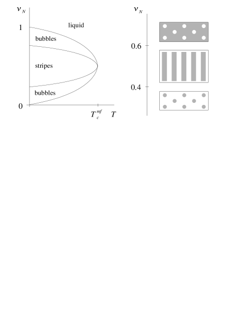
Figure 1: Left: Mean-field phase diagram. Right: Guiding center density domain patterns at $T=0$. Shaded and blank areas symbolize filled and empty regions, respectively.

The mean-field theory is expected to be valid in the quasiclassical limit of large $N$. At moderate $N$ the CDW compete with Laughlin liquids and other fractional quantum Hall (FQH) states. A combination of analytic and numerical tools $\!{}^{{\bf?},{\bf?},{\bf?},{\bf?},{\bf?}}$ suggests that the FQH states lose to the CDW at $N\geq 2$.

The existence of the stripe phase as a physical reality was evidenced by a conspicuous magnetoresistance anisotropy observed near half-integral fractions of high LLs $\!{}^{{\bf?},{\bf?},{\bf?}}$ (see Ref. 13 for review). This anisotropy develops at $T<0.1\,{\rm K}$ in high-mobility samples. The anisotropy is the largest at total filling factor $\nu=9/2$ ($N=2$, $\nu_{N}=1/2$) and decreases with increasing LL index. At $T=25\,{\rm mK}$ it remains discernible up to $\nu\sim 11\frac{1}{2}$ whereupon it is washed out, presumably, due to disorder and finite temperature. The anisotropy is natural once we assume that the stripe phase forms. The edges of the stripes can be visualized as metallic rivers, along which the transport is “easy.” The charge transfer among different edges, i.e., across the stripes, requires quantum tunneling and is “hard” because the stripes are effectively far away.

The existence of the bubble phases at high LLs is supported by the discovery of reentrant integral quantum Hall effect (IQHE) at $\nu\approx 4.25$ and $\nu\approx 4.75$. The Hall resistance at such filling factors is quantized at the value of the nearest IQHE plateau, while the longitudinal resistance is isotropic and shows a deep minimum with an activated temperature dependence. The current-voltage ($I$-$V$) characteristics exhibit pronounced nonlinearity, switching, and hysteresis. These observations are consistent with the theoretical picture of a bubble lattice pinned by disorder.

2 Liquid crystal analogy for the stripe phase

In the wake of the experiments, a considerable amount of work has been devoted to the stripe phase in recent years, Refs. 14–27. It led to the understanding that the “stripes” may appear in several distinct forms: an anisotropic crystal, a smectic, a nematic, and an isotropic liquid (Fig. 2). These phases succeed each other in the order listed as the magnitude of either quantum or thermal fluctuations increases. Consequently, the phase diagram of Fig. 1 needs modifications to incorporate some of those phases. The general structure of the revised phase diagram for the quantum ($T=0$) case was discussed in the important paper of Fradkin and Kivelson. $\!{}^{{\bf?}}$ However, pinpointing the new phase boundaries in terms of the conventional parameters $r_{s}$, $\nu$, and $T$ requires further work. The most intriguing are the phases which bear the liquid crystal names: the smectic and the nematic. They are the main subject of this report. Let us start with the basic definitions of these phases.

The smectic is a liquid with the 1D periodicity, i.e., a state where the translational symmetry is spontaneously broken in one spatial direction. $\!{}^{{\bf?}}$ The rotational symmetry is of course broken as well. An example of such a state is the original Hartree-Fock stripe solution $\!{}^{{\bf?}}$ although a stable quantum Hall smectic must have a certain amount of quantum fluctuations around the mean-field state. $\!{}^{{\bf?},{\bf?}}$ The necessary condition for the smectic order is the continuity of the stripes. If the stripes are allowed to rupture, the dislocations are created. They destroy the 1D positional order and convert the smectic into the nematic. $\!{}^{{\bf?}}$

By definition, the nematic is an anisotropic liquid. $\!{}^{{\bf?}}$ There is no long-range positional order. As for the orientational order, it is long-range at $T=0$ and quasi-long-range (power-law correlations) at finite $T$. The nematic is riddled with dynamic dislocations. Other types of topological defects, the disclinations, may also be present but remain bound in pairs, much like vortices in the 2D $X$-$Y$ model. Once they unbind, all the spatial symmetries are restored. The resultant state is an isotropic liquid with short-range stripe correlations. As the fluctuations due to temperature or quantum mechanics increase further, it gradually crosses over to the “uncorrelated liquid” where even the local stripe order is obliterated.

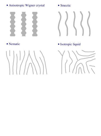
Figure 2: Sketches of possible stripe phases.

It is often the case that the low-frequency long-wavelength physics of the system is governed by an effective theory involving a relatively small number of dynamical variables. In the remaining sections we will discuss such type of theories for the quantum Hall liquid crystals.

3 Smectic state

Effective theory.— The collective variables in the smectic are (i) the deviations $u(x,y)$ of the stripes from their equilibrium positions and (ii) long-wavelength density fluctuations $n$ about the average value $n_{0}$. The latter fluctuations may originate, e.g., from width fluctuations of the stripes. Let us assume that the stripes are aligned in the $\hat{\bf y}$-direction, then the symmetry considerations fix the effective Hamiltonian for $u$ and $n$ to be $\!{}^{{\bf?},{\bf?}}$

$$H=\frac{Y}{2}\Bigl{[}\partial_{x}u-\frac{1}{2}(\nabla u)^{2}\Bigr{]}^{2}+\frac{K}{2}(\partial_{y}^{2}u)^{2}+\frac{1}{2}nUn,$$ (1)

where $Y$ and $K$ are the phenomenological compression and the bending elastic moduli, and $U(r)=e^{2}/\kappa r$ should be understood as the integral operator. The dynamics of the smectic is dominated by the Lorentz force and is governed by the Largangean

$${\cal L}=p\partial_{t}u-H,\quad\partial_{y}p=-m\omega_{c}(n+n_{0}\partial_{x}u),$$ (2)

where $m$ is the electron mass and $\omega_{c}=eB/mc$ is the cyclotron frequency.

From Eqs. (1) and (2) we can derive the spectrum of collective modes, the magnetophonons. It is natural to start with the harmonic approximation where one replaces the first term in $H$ simply by $(Y/2)(\partial_{x}u)^{2}$. Solving the equations of motion for $n$ and $u$ we obtain the magnetophonon dispersion relation: $\!{}^{{\bf?}}$

$$\omega({\bf q})=\frac{\omega_{p}(q)}{\omega_{c}}\frac{q_{y}}{q}\left[\frac{Yq_{x}^{2}+Kq_{y}^{4}}{mn_{0}}\right]^{1/2}.$$ (3)

Here $\omega_{p}(q)=[n_{0}U(q)q^{2}/m]^{1/2}$ is the plasma frequency and $\theta=\arctan(q_{y}/q_{x})$ is the angle between the propagation direction and the $\hat{\bf x}$-axis. For Coulomb interactions $\omega_{p}(q)\propto\sqrt{q}$. Unless propagate nearly parallel to the stripes, $\omega({\bf q})$ is proportional to $\sin 2\theta\,q^{3/2}$. One immediate consequence of this dispersion is that the largest velocity of propagation for the magnetophonons with a given $q$ is achieved when $\theta=45^{\circ}$.

Thermal fluctuations and anharmonisms.— From Eq. (1) we can readily calculate the mean-square fluctuations of the stripe positions at finite $T$, e.g.,

$$\langle[u(0,0)-u(0,y)]^{2}\rangle=\frac{k_{B}T}{2\sqrt{YK}}|y|.$$ (4)

As one can see, at any finite temperature magnetophonon fluctuations are growing without a bound; hence, the positional order of a 2D smectic is totally destroyed $\!{}^{{\bf?}}$ at sufficiently large distances along the $\hat{\bf y}$-direction, $|y|\gg\Lambda\sqrt{YK}/k_{B}T\equiv\xi_{y}$ where $\Lambda=2\pi/q_{*}$ is the interstripe separation. Similarly, along the $\hat{\bf x}$-direction, the positional order is lost at lengthscales larger than $\xi_{x}=(Y/K)^{1/2}\xi_{y}^{2}$.

Another type of excitations, which disorder the stripe positions are the aforementioned dislocations. The dislocations in a 2D smectic have a finite energy $E_{D}\sim K$. At $k_{B}T\ll E_{D}$ the density of thermally excited dislocations is of the order of $\exp(-E_{D}/k_{B}T)$ and the average distance between dislocations is $\xi_{D}\sim\Lambda\exp(2k_{B}T/E_{D})$. At low temperatures $\xi_{x},\xi_{y}\ll\xi_{D}$; therefore, the following interesting situation emerges (Fig. 3). On the lengthscales smaller than $\xi_{y}$ (or $\xi_{x}$, whichever appropriate) the system behaves like a usual smectic where Eqs. (1–3) apply. On the lengthscales exceeding $\xi_{D}$ it behaves like a nematic. $\!{}^{{\bf?}}$ In between the system is a smectic but with very unusual properties. It is topologically ordered (no dislocations) but possesses enormous fluctuations. In these circumstances the harmonic elastic theory becomes inadequate and anharmonic terms must be treated carefully.

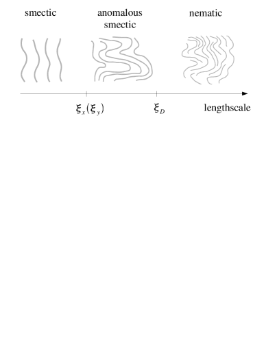
Figure 3: Portraits of the stripe phase on different lengthscales.

As shown by Golubović and Wang, $\!{}^{{\bf?}}$ the anharmonisms cause power-law dependence of the parameters of the effective theory on the wavevector ${\bf q}$:

$$Y\sim Y_{0}(\xi_{y}q_{y})^{1/2},\quad K\sim K_{0}(\xi_{y}q_{y})^{-1/2},$$ (5)

for $q_{x}\ll\xi_{x}^{-1}(q_{y}\xi_{y})^{3/2}$, $q_{y}\ll\xi_{y}^{-1}$, and

$$Y\sim Y_{0}(\xi_{x}q_{x})^{1/3},\quad K\sim K_{0}(\xi_{x}q_{x})^{-1/3},$$ (6)

for $q_{x}\ll\xi_{x}^{-1}$ and $q_{y}\ll\xi_{y}^{-1}(q_{x}\xi_{x})^{2/3}$. The lengthscale dependence of the parameters of the effective theory is a common feature of fluctuation-dominated phenomena. It should be mentioned that the lower critical dimension for the smectic order is $d=3$, $\!{}^{{\bf?}}$ so that the 2D smectic is below its lower critical dimension. This is the reason why the scaling behavior (5) and (6) does not persist indefinitely but eventually breaks down above the lengthscale $\xi_{D}$ where the crossover to the thermodynamic limit of the nematic behavior commences.

The scaling shows up not only in the static properties such as $Y$ and $K$ but also in the dynamics. The role of anharmonisms in the dynamics of conventional 3D smectics has been investigated by Mazenko et al. $\!{}^{{\bf?}}$ and also by Kats and Lebedev $\!{}^{{\bf?}}$. For the quantum Hall stripes the analysis had to be done anew because here the dynamics is totally different. It is dominated by the Lorentz force rather than a viscous relaxation in the conventional smectics. This task was accomplished in Ref. 17. The calculation was based on the Martin-Siggia-Rose formalism combined with the $\epsilon$-expansion below $d=3$ dimensions. One set of results concerns the spectrum of the magnetophonon modes, which becomes

$$\omega({\bf q})\sim\sin\theta\cos^{7/6}\theta\,(\xi_{x}q)^{5/3}\frac{\omega_{p}(\xi_{x}^{-1})}{\omega_{c}\xi_{x}}\sqrt{\frac{Y_{0}}{mn_{0}}}.$$ (7)

Compared to the predictions of the harmonic theory, Eq. (3), the $q^{3/2}$-dispersion changes to $q^{5/3}$. Also, the maximum propagation velocity is achieved for the angle $\theta\approx 53^{\circ}$ instead of $\theta=45^{\circ}$. These modifications, which take place at long wavelengths, are mainly due to the renormalization of $Y$ in the static limit and can be obtained by combining Eqs. (3) and (6). Less obvious dynamical effects peculiar to the quantum Hall smectics include a novel dynamical scaling of $Y$ and $K$ as a function of frequency and a specific $q$-dependence of the magnetophonon damping. $\!{}^{{\bf?}}$

The latter issue touches on an important point. Our effective theory defined by Eqs. (1) and (2) is based on the assumption that $u$ and $n$ are the only low-energy degrees of freedom. It is probably well justified at $T\rightarrow 0$ but becomes incorrect at higher temperatures. The point of view taken in Ref. 17 is that in the latter case thermally excited quasiparticles (“normal fluid”) should appear and that they should bring dissipation into the dynamics of the magnetophonons. Another intriguing possibility is for quasiparticles or other additional low-energy degrees of freedom to exist even at $T=0$. Such more complicated smectic states are interesting subjects for future study.

4 Nematic

As discussed above, at finite temperature and in the thermodynamic limit, the smectic phase is always unstable. The lowest degree of ordering is that of a nematic. $\!{}^{{\bf?}}$ An intriguing possibility $\!{}^{{\bf?}}$ is to have a nematic phase already at $T=0$, due to quantum fluctuations. The collective degree of freedom associated with the nematic ordering is the angle $\phi({\bf r},t)$ between the local normal to the stripes ${\bf N}$ and the $\hat{\bf x}$-axis orientation. The effective Hamiltonian for ${\bf N}$ is dictated by symmetry to be

$$H_{N}=\frac{K_{1}}{2}(\nabla{\bf N})^{2}+\frac{K_{3}}{2}|\nabla\times{\bf N}|^{2}.$$ (8)

The phenomenological coefficients $K_{1}$ and $K_{3}$ are termed the splay and the bend Frank constants. $\!{}^{{\bf?}}$ A particularly simple form is obtained if $K_{1}=K_{3}$, in which case $H_{N}=(K_{3}/2)(\nabla\phi)^{2}$ just like in the $X$-$Y$ model.

Another obvious degree of freedom in the nematic are the density fluctuations $n({\bf r},t)$. A peculiar fact is that in the static limit $n$ is totally decoupled from ${\bf N}$, and so it does not enter Eq. (8). However, since the nematic is less ordered than even a smectic, the question about extra low-energy degrees of freedom or additional quasiparticles is highly relevant. We believe that different types of quantum Hall nematics are possible in nature. In the simplest case scenario ${\bf N}$ and $n$ are the only low-energy degrees of freedom. This is presumably the case when the nematic order is a superstructure on top of a parent uniform state. A concrete example is described by a wavefunction proposed by Musaelian and Joynt: $\!{}^{{\bf?}}$

$$\Psi=\prod\limits_{j<k}(z_{j}-z_{k})[(z_{j}-z_{k})^{2}-a^{2}]\times\exp\Bigl{(}-\sum_{j}|z_{j}|^{2}/4l^{2}\Bigr{)}.$$ (9)

Here $z_{j}=x_{j}+iy_{j}$ is a complex coordinate of $j$th electron, $l=\sqrt{\hbar c/eB}$ is the magnetic length, and $a$ is another complex parameter that determines the degree of orientational order and the direction of the stripes. The rotational invariance is broken if $|a|$ exceeds some critical value. This particular wavefunction corresponds to $\nu=\frac{1}{3}$ but can be easily generalized to higher Landau levels with $\nu_{N}=\frac{1}{3}$ filling. This type of state has been studied by Balents $\!{}^{{\bf?}}$ and recently by the present author. $\!{}^{{\bf?}}$ It was essentially postulated that the effective Largangean takes the form

$${\cal L}=\frac{1}{2}\gamma^{-1}(\partial_{t}{\bf N})^{2}-H.$$ (10)

(As hinted above, the full expression contains also couplings between $\partial_{t}{\bf N}$ and mass currents but they become vanishingly small in the long-wavelength limit). The collective excitations are charge-neutral fluctuations of the director. They have a linear dispersion,

$$\omega({\bf q})=q\sqrt{{K_{1}}{\gamma}\cos^{2}\theta+{K_{3}}{\gamma}\sin^{2}\theta},$$ (11)

and resemble spinwaves in the $X$-$Y$ quantum rotor model.

The quantum nematic phase must be separated from the stable zero-temperature smectic by a quantum phase transition. Further insights into the properties of the quantum nematics can be gained by analyzing the nature of such a transition. By analogy to the classical smectic-nematic transition in two $\!{}^{{\bf?}}$ and three $\!{}^{{\bf?}}$ dimensions, we expect the quantum one to also be driven by the proliferation of dislocations. Pictorially, the difference between the smectic and nematic can be represented as follows. The dislocations are viewed as lines in the (2 + 1)D space. In the smectic phase, they form small closed loops (Fig. 4a) that depict virtual pair creation-annihilation events; in the nematic phase arbitrarily long dislocation worldlines exist and may entangle (Fig. 4b), similar to worldlines of particles in a Bose superfluid.

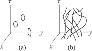
Figure 4: Worldlines of dislocations in (a) smectic (b) nematic.

To incorporate the dislocations into the effective Lagrangean (2), we use a well known duality transformation, see, for example, Ref. 34. By means of such a transformation the original degrees of freedom $u$ and $n$ are traded for new variables: the second-quantized dislocation field $\Phi$ and an auxillary $U(1)$ gauge field $a_{\mu}$, which mediates the interaction among the dislocations. The imaginary-time effective action for $\Phi$ and $a_{\mu}$ has the form

$$A = \int\limits_{0}^{\beta}d\tau\int d^{2}{\bf r}\biggl{\{}\frac{t_{\mu}}{2}|(-i\partial_{\mu}-\Lambda a_{\mu}-e_{D}a_{\mu}^{\rm ext})\Phi|^{2}\biggr{.}$$ (12)

$$+ \biggl{.}V(\Phi)+H_{a}[a]\biggr{\}},$$

$$H_{a} = \frac{\sigma_{x}^{2}}{2Y}+\sigma_{y}(-2K\partial_{y}^{2})^{-1}\sigma_{y}+\frac{l^{4}}{2}\partial_{y}\sigma_{\tau}U\partial_{y}\sigma_{\tau},$$ (13)

$$\sigma_{\mu} = \epsilon_{\mu\nu\lambda}\partial_{\nu}a_{\lambda}\equiv[\partial\times a]_{\mu}.$$ (14)

Phenomenological parameters introduced above are as follows. Parameter $t_{\tau}$ is of the order of $\hbar^{2}/E_{c}$, where $E_{c}$ is the dislocation core energy estimated within the Hartree-Fock approximation in Refs. 4 and 21. Unfortunately, this estimate is not reliable in the quantum nematic state where the quantum fluctuations are large. Parameter $t_{x}$ of dimension of ${\rm energy}\times{\rm(length)}^{2}$ is the hopping matrix element for dislocation motion in the $\hat{\bf x}$-direction, i.e., dislocation glide. Such a glide requires quantum tunneling and is exponentially small unless $\Lambda<l$. Parameter $t_{y}$ describes the dislocation climb, which also originates from the dynamics on the microscopic length scales. Yet another phenomenological variable is the potential $V(\Phi)=m_{\Phi}|\Phi|^{2}+r_{\Phi}|\Phi|^{4}+\ldots$, which accounts for a self-energy and a short-range interaction between the dislocations; the scales of $m_{\Phi}$ and $r_{\Phi}$ are set by $E_{c}$ and $E_{c}\Lambda^{2}$, respectively. Finally, $e_{D}$ is electric charge of the dislocation that couples to the external vector potential $a_{\tau}^{\rm ext}=a_{x}^{\rm ext}=0$, $a_{y}^{\rm ext}=Bx$. This coupling is introduced only for the sake of generality. Since we study electron liquid crystal phases derived from incompressible liquids, we expect dislocations to be electrically neutral, i.e., $e_{D}=0$.

To recover Eq. (11) we assume that the dislocations have condensed, $\langle\Phi\rangle=\Phi_{0}\neq 0$. Solving for the collective mode spectrum of the action (12), we find

$$\omega_{1}({\bf q})=\left(\frac{m_{x}}{m_{\tau}}q_{x}^{2}+m_{x}Kq_{y}^{2}\right)^{1/2},\>\>m_{\mu}\equiv t_{\mu}\Lambda^{2}|\Phi_{0}|^{2},$$ (15)

which is consistent with Eq. (11) if $K_{1}=1/m_{\tau}$, $K_{3}=K$, and $\gamma=m_{x}$.

Remarkably, the magnetophonon mode of the parent smectic (3), does not totally disappear from the spectrum. Instead, it acquires a small gap $\sqrt{m_{y}Y}$ at $q=0$. This gapped mode anti-crosses with the acoustic branch (15) near the point $\omega_{1}^{2}({\bf q})\sim m_{y}Y$, and at larger $q$ becomes the lowest frequency collective mode with the dispersion relation

$$\omega_{2}({\bf q})=\left[\frac{q^{2}_{x}q^{2}_{y}}{m^{2}\omega_{c}^{2}}YU(q)+m_{y}Y\right]^{1/2}$$ (16)

only slightly different from (3). At such $q$ the structure factor of the nematic has two sets of $\delta$-functional peaks,

$$S(\omega,{\bf q})=\frac{\pi\hbar q_{y}^{2}}{m\omega_{c}^{2}}\left[\frac{Kq_{y}^{4}}{mn_{0}}\delta(\omega^{2}-\omega_{1}^{2})+\frac{Yq_{x}^{2}}{mn_{0}}\delta(\omega^{2}-\omega_{2}^{2})\right],$$

which split between themselves the spectral weight of the single collective mode of the smectic. The presence of the two modes can be explained by the existence of two order parameters: the aforementioned unit vector (more precisely, director) ${\bf N}$ normal to the local stripe orientation and the complex wavefunction $\Phi_{0}$ of the dislocation condensate. Classical 2D nematics have two (overdamped) modes virtually for the same reason. $\!{}^{{\bf?}}$

Recently, Radzihovsky and Dorsey $\!{}^{{\bf?}}$ formulated a qualitatively different theory of the quantum Hall nematics, whose predictions disagree with our Eqs. (10) and (11). At this point it is unclear whether these authors study a different kind of nematic or they actually contest the theoretical models proposed by Balents $\!{}^{{\bf?}}$ and the present author. $\!{}^{{\bf?}}$ To resolve some of these issues it is imperative to bring the discussion from the level of effective theory to the level of quantitative calculations. One promising direction is to investigate some concrete trial wavefunctions of quantum nematics, e.g., Eq. (9). Recently, the work in this direction was continued by Ciftja nad Wexler. $\!{}^{{\bf?}}$ It is also desirable to find a functional form of the electron-electron interaction which gives rise to the nematic ground state. An educated guess $\!{}^{{\bf?}}$ is that even a realistic Coulomb interaction may be sufficient provided $r_{s}\ll 1$ and $1\ll N\ll r_{s}^{-2}$. However, the quest for quantum nematic may not be easy. Finite-size study by Rezayi et al. $\!{}^{{\bf?}}$ suggests that the transition from the smectic to an isotropic phase as a function of the interaction parameters (Haldane’s pseudopotentials) can also occur via a first-order transition, without the intermediate nematic phase.

Experimentally, the nematic can be distinguished from the smectic by, e.g., the microwave absorption technique: the nematic will show two dispersing collective modes while the smectic will produce a single one. To circumvent disorder pinning effects, such measurements should be done at high enough $q$.

References

References

- [1] For review, see Quantum Hall Effect edited by R. E. Prange and S. M. Girvin (Springer-Verlag, New York, 1990); Perspectives in Quantum Hall Effect edited by S. Das Sarma and A. Pinczuk (Wiley, New York, 1997).
- [2] For review, see M. M. Fogler, cond-mat/0111001.
- [3] I. L. Aleiner and L. I. Glazman, Phys. Rev. B52, 11 296 (1995).
- [4] A. A. Koulakov, M. M. Fogler, and B. I. Shklovskii, Phys. Rev. Lett. 76, 499 (1996); M. M. Fogler, A. A. Koulakov, and B. I. Shklovskii, Phys. Rev. B54, 1853 (1996).
- [5] H. Fukuyama, P. M. Platzman, and P. W. Anderson, Phys. Rev. B19, 5211 (1979).
- [6] M. M. Fogler and A. A. Koulakov, Phys. Rev. B55, 9326 (1997).
- [7] R. Moessner and J. T. Chalker, Phys. Rev. B54, 5006 (1996).
- [8] E. H. Rezayi, F. D. M. Haldane, and K. Yang, Phys. Rev. Lett. 83, 1219 (1999); ibid 85, 5396 (2000).
- [9] N. Shibata and D. Yoshioka, Phys. Rev. Lett. 86, 5755 (2001).
- [10] M. P. Lilly, K. B. Cooper, J. P. Eisenstein, L. N. Pfeiffer, and K. W. West, Phys. Rev. Lett. 82, 394 (1999).
- [11] R. R. Du, D. C. Tsui, H. L. Störmer, L. N. Pfeiffer, and K. W. West, Solid State Commun. 109, 389 (1999).
- [12] M. Shayegan, H. C. Manoharan, S. J. Papadakis, and E. P. DePoortere, Physica E 6, 40 (2000).
- [13] J. P. Eisenstein, M. P. Lilly, K. B. Cooper, L. N. Pfeiffer, and K. W. West, Physica E 9, 1 (2001); J. P. Eisenstein, Solid State Commun. 117, 132 (2001).
- [14] E. Fradkin and S. A. Kivelson, Phys. Rev. B59, 8065 (1999).
- [15] A. H. MacDonald and M. P. A. Fisher, Phys. Rev. B61, 5724 (2000).
- [16] H. A. Fertig, Phys. Rev. Lett. 82, 3693 (1999).
- [17] M. M. Fogler and V. M. Vinokur, Phys. Rev. Lett. 84, 5828 (2000).
- [18] R. Côté and H. A. Fertig, Phys. Rev. B62, 1993 (2000).
- [19] H. Yi, H. A. Fertig, and R. Côté, Phys. Rev. Lett. 85, 4156 (2000).
- [20] M. M. Fogler, cond-mat/0107306.
- [21] C. Wexler and A. T. Dorsey, Phys. Rev. B64, 115 312 (2001).
- [22] D. G. Barci, E. Fradkin, S. A. Kivelson, and V. Oganesyan, cond-mat/0105448.
- [23] A. Lopatnikova, B. I. Halperin, S. H. Simon, and X.-G. Wen, cond-mat/0105079.
- [24] K. Musaelian and R. Joynt, J. Phys. Cond. Mat. 8, L105 (1996).
- [25] L. Balents, Europhys. Lett. 33, 291 (1996).
- [26] O. Ciftja and C. Wexler, cond-mat/0108119.
- [27] L. Radzihovsky and A. T. Dorsey, cond-mat/0110083.
- [28] P. G. de Gennes and J. Prost, The Physics of Liquid Crystals (Oxford University Press, New York, 1995).
- [29] J. Toner and D. R. Nelson, Phys. Rev. B23, 316 (1981).
- [30] L. Golubović and Z.-G. Wang, Phys. Rev. Lett. 69, 2535 (1992).
- [31] G. F. Mazenko, S. Ramaswamy, and J. Toner, Phys. Rev. Lett. 49, 51 (1982); Phys. Rev. A28, 1618 (1983).
- [32] E. I. Kats and V. V. Lebedev, Fluctuational Effects in The Dynamics of Liquid Crystals (Springer-Verlag, New York, 1994).
- [33] J. Toner, Phys. Rev. B26, 462 (1982); A. R. Day, T. C. Lubensky, and A. J. McKane, Phys. Rev. A27, 1461 (1983).
- [34] M. P. A. Fisher and D. H. Lee, Phys. Rev. B39, 2756 (1989).
- [35] E. H. Rezayi and F. D. M. Haldane, Phys. Rev. Lett. 84, 4685 (2000).