Mean-field approach to ferromagnetism in (III,Mn)V diluted magnetic semiconductors at low carrier densities

Abstract

We present a detailed study, within the mean-field approximation, of an impurity band model for III-V diluted magnetic semiconductors. Such a model should be relevant at low carrier densities, below and near the metal-insulator transition. Positional disorder of the magnetic impurities inside the host semiconductor is shown to have observable consequences for the shape of the magnetization curve. Below the critical temperature the magnetization is spatially inhomogeneous, leading to very unusual temperature dependence of the average magnetization as well as specific heat. Disorder is also found to enhance the ferromagnetic transition temperature. Unusual spin and charge transport is implied.

]

I Introduction

Diluted magnetic semiconductors (DMS) are semiconductors of the general type A_1-xM_xB, where AB is either a II-VI or a III-V semiconductor and M a magnetic element, most commonly Mn. Substitution of a small fraction $x$ of the element A by Mn impurities (and in the case of II-VI semiconductors an additional charge dopant, such as P on the B site) leads to the emergence of a semiconductor with ferromagnetic properties.[1] This is due to the interactions of the $S={5\over 2}$ Mn spins (coming from the half-filled 3d shell of the Mn) with the spins of the charge carriers introduced by the Mn dopants, or, in the case of II-VI semiconductors, by the additional dopant. This opens up the possibility of manipulating (through doping) not only the charge, but also the spin properties of the semiconductor. The ability to control the properties of a system by acting on the spin of its charge carriers is the subject of the new field of “spintronics”, and is believed to hold the promise to developing devices which combine storage functionalities (such as memory devices) together with information processing functionalities.

The recent demonstration of Curie temperatures of the order of 100 K in Ga_1-xMn_xAs samples with $x\approx 0.05$, grown at low-temperatures using molecular-beam epitaxy (MBE) techniques, [2, 3, 4] has heightened the interest in understanding the physics of these alloys. By now, it is well established that the main magnetic interaction is an antiferromagnetic (AFM) exchange between the Mn spins and the charge carrier spins. As a result, an effective ferromagnetic (FM) interaction arises between the Mn spins through carrier-induced ferromagnetism. Several theories, most notably Ruderman-Kittel-Kasuya-Yosida (RKKY),[5] have been used to explain, within a mean-field approximation, this phenomenon. More recently, dynamic correlations as well as arbitrary itinerant-carrier spin polarizations have been included.[6] However, all these models assume that the charge carriers (the holes) occupy a Fermi sea in the valence band. This implicitly assumes a spatially homogeneous distribution of the holes throughout the entire system, and therefore completely neglects the role of the Coulomb attraction between the charge carriers and the Mn ions, as well as the role of disorder which is always present in such alloy systems.

It is well known [7] that Mn impurities in a III-V semiconductor create a trapping potential for holes. The associated acceptor levels are about 100 meV above the top of the valence band, for GaAs, and interactions will lead to their splitting into an impurity band.[8, 9] At $T=0$, the holes occupy the states of lowest energy and therefore they first occupy states in the impurity band. Only if the Fermi energy (or thermal energy $k_{B}T$) is large enough are states in the valence band occupied as well. It has been found experimentally that these alloys are heavily compensated, leading to rather small hole concentrations, of the order of 10% of the Mn concentration.[10] The corresponding small Fermi energy implies a long screening length for the Coulomb interactions, and opens up the possibility that holes are actually moving (through hopping processes) in the impurity band formed of states localized about the Mn impurities. Strong experimental evidence for this scenario comes from electrical conductivity measurements, which at low temperatures reveal Mott variable-range hopping behavior. [4, 11] As a result, randomness in the position of the Mn spins (and associated random potential) could be expected to play an important role.

In this paper we investigate, at the mean-field level, a model in which holes move in a band formed of impurity states, neglecting the existence of the valence band states. Some results of this model have already been reported in Ref. 12. While a complete model should include both impurity and valence band states, we believe that our model is a good first approximation, especially at low temperatures, since we find typical Fermi energies of a few tens of meV, smaller than the average $\sim 100$meV between the impurity band and the valence band.

The paper is organized as follows. In Section II we describe the model Hamiltonian, the self-consistent mean-field approximation as well as the specific parameters used in the numerical calculations. It is important to emphasize that although we chose numbers from the literature specific to the GaMnAs problem for illustration purposes, similar arguments and physics would hold for other III-V compounds. In Section III we present our results. We first analyze the hypothetical case in which all Mn impurities are ordered in a simple cubic lattice. This allows us to understand the unusual shape of the magnetization curves we obtain. More importantly, it allows us to clearly identify the non-trivial effects of randomness (disorder) in the Mn positions. These are analyzed in some detail and a clear physical picture of their importance to the problem emerges. We also analyze the metal-insulator transition, the effects of on-site random disorder, as well as other possible interactions. The sensitivity of our results to variations in the impurity band parameters is also discussed. Finally, Section IV contains a summary and conclusions.

II Model

Based on experimental work in the literature,[1] we assume that Mn only substitutes for the group III element of the III-V semiconductor. The III-V semiconductor is assumed to have a zinc-blende structure. Let $\vec{R}_{i},i=1,...,N_{d}$ be the random positions of the $N_{d}$ Mn dopants in the face centered cubic (FCC) sublattice of the group III element. Each Mn impurity is associated with a spin-${5\over 2}$ from its half-filled $3d$ shell. Since Mn has nominal valence II, when it substitutes for the valence-III element it will act as an acceptor. As a result, it can trap a hole shallow level, characterized by a hydrogenic Bohr radius $a_{B}$. Let $N_{h}$ be the total number of holes trapped about various Mn sites, and $p=N_{h}/N_{d}$ the relative hole concentration. A hole can hop from one Mn impurity to another one, while its spin is antiferromagnetically coupled to the Mn spins in its vicinity.

For simplicity, although the charge carriers of this system are holes, in the following we use an “electron”-formalism to analyze them. In other words, we in fact analyze an equivalent system doped with hypothetical donors, with impurity levels below a conduction-like band, instead of being above a valence-like band. The main difference between the two models is (i) the hole spin is ${3\over 2}$ and (ii) the envelope wave function of hole has cubic symmetry, rather than spherical symmetry of a donor. This leads to some quantitative differences (as has been shown by MacDonald and coworkers for free holes in Ref. 13) but the essential aspects of the problem, namely (a) disorder and (b) the effect of impurity potentials, which we concentrate on here, remain substantially unaffected.

The Hamiltonian we study is:

$${\cal H}=\sum_{i,j}t_{ij}c^{\dagger}_{i\sigma}c_{j\sigma}+\sum_{i}u(i)c^{\dagger}_{i\sigma}c_{i\sigma}$$

$$+\sum_{i,j}J_{ij}\vec{S}(i)\left(c^{\dagger}_{j\alpha}{1\over 2}\vec{\sigma}_{\alpha\beta}c_{j\beta}\right)$$

$$-g\mu_{B}H\sum_{i}{\sigma\over 2}c^{\dagger}_{i\sigma}c_{i\sigma}-\tilde{g}\mu_{B}H\sum_{i}S^{z}(i).$$ (1)

Here, $c^{\dagger}_{i\sigma}$ is the creation operator of a charge carrier with spin $\sigma$ in the bound orbital associated with the $i$th Mn impurity. The first term in Eq. (1) describes charge carriers hopping between various Mn sites, with the hopping matrix $t_{ij}$ dependent on the hopping distance $r=|\vec{R}_{i}-\vec{R}_{j}|$. We take an exponential form like for hydrogenic orbitals $t(r)=2\left(1+{r/a_{B}}\right)\exp{\left(-{r/a_{B}}\right)}\mbox{ Ry}$. [14] We present detailed results for this case; however we discuss in subsection F the changes that result with other models of the hopping integral. From these different cases we discern the universal aspects of the impurity models and also the requisite conditions for the existence of the experimentally observed ferromagnetism.

The Rydberg (Ry) is defined by the binding energy of the charge carrier to the shallow trap, $E_{b}$. The heavily compensated nature of the system gives rise to random potentials coming from the charged centers responsible for compensation. We model this through an on-site random potential $u(i)$ which leads to the second term in Eq. 1. A full model would require a self-consistent determination of this potential taking in consideration screening processes. The third term is the AFM interaction between Mn spins $\vec{S}(i)$ and charge carrier spins. Since the Mn spins are very localized (the $3d$ shell has a radius of the order 1-2Å) the antiferromagnetic exchange integral is taken to be of the form $J_{ij}=J|\phi(i,j)|^{2}=J\exp{\left(-2{|\vec{R}_{i}-\vec{R}_{j}|/a_{B}}\right)}$, reflecting the probability of finding the charge carrier in the $s$-type shallow level about impurity $j$ near the $i$th Mn spin. In this notation, $J$ is simply the AFM exchange integral of an isolated localized hole centered at a Mn impurity with the spin of the Mn. The last line in Eq. (1) describes the interaction of the carrier and Mn spins with an external magnetic field H.

A Mean-Field Approximation

We treat the antiferromagnetic interaction at the mean-field level, given by the factorization

$$\vec{S}(i)\cdot\hat{\vec{\sigma}}_{j}\rightarrow S_{Mn}(i)\hat{\sigma^{z}_{j}}+S^{z}(i)s_{h}(j)-S_{Mn}(i)s_{h}(j),$$ (2)

where $S_{Mn}(i)=\langle S^{z}(i)\rangle$ and $s_{h}(j)=\langle{\hat{\sigma}}^{z}_{j}\rangle$ are the expectation values of the $i$th Mn spin and of the total spin created by charge carriers at the $j$th Mn site, respectively, and must be computed self-consistently at each site. For simplicity of notation, we used $\hat{\vec{\sigma}}_{j}=c^{\dagger}_{j\alpha}{1\over 2}\vec{\sigma}_{\alpha\beta}c_{j\beta}$ in Eq. (2). In writing Eq. (2) we made the implicit assumption that the rotational symmetry is broken in the direction of the external magnetic field H (defining the z-axis) for all spins. In fact, one may start with a Heisenberg-like factorization in the absence of external magnetic fields, but we find that in the self-consistent configurations the spins are always collinear, and as a result we regain the Ising-like factorization of Eq. (2). Disorder induced non-collinear ground-states have been recently suggested in a model which assumes that holes occupy a Fermi sea in the valence band. [15]

The mean-field Hamiltonian can be separated into three parts

$${\cal H}_{MF}={\cal H}_{spin}+{\cal H}_{cc}+{\cal H}_{const}.$$ (3)

The spin Hamiltonian may be rewritten as

$${\cal H}_{spin}=-\sum_{i}H_{i}S^{z}(i),$$ (4)

where

$$H_{i}=\tilde{g}\mu_{B}H-J\sum_{j}|\phi(i,j)|^{2}s_{h}(j)$$ (5)

is the effective magnetic field for the Mn spin at site $i$, including the charge carrier contributions. Then, the average Mn spin at site $i$ is

$$S_{Mn}(i)={\cal B}_{S}(\beta H_{i}),$$ (6)

where ${\cal B}_{S}(x)=(S+{1\over 2})\coth{[(S+{1\over 2})x]}-{1\over 2}\coth{{x\over 2}}$ is the Brillouin function corresponding to the spin $S=5/2$, and $\beta=1/k_{B}T$. The contribution to the internal energy from the spin Hamiltonian equals

$$U_{spin}(T)=-\sum_{i}H_{i}S_{Mn}(i).$$ (7)

The charge carrier Hamiltonian can be rewritten as

$${\cal H}_{cc}=\sum_{i,j}t_{ij}c^{\dagger}_{i\sigma}c_{j\sigma}+\sum_{i\sigma}\left(\epsilon_{i\sigma}-\mu\right)c^{\dagger}_{i\sigma}c_{i\sigma},$$ (8)

where

$$\epsilon_{i\sigma}={\sigma\over 2}\left(J\sum_{j}|\phi(i,j)|^{2}S_{Mn}(j)-g\mu_{B}H\right)+u(i)$$ (9)

is the effective on-site energy created by the Mn spins, the on-site disorder and the external magnetic field. A chemical potential $\mu$ has been added since we treat the charge carriers in the grand-canonical ensemble.

The charge carrier Hamiltonian can be diagonalized to obtain:

$${\cal H}_{cc}=\sum_{n\sigma}(E_{n\sigma}-\mu)a^{\dagger}_{n\sigma}a_{n\sigma},$$ (10)

using the linear combinations

$$a^{\dagger}_{n\sigma}=\sum_{i}\psi_{n\sigma}(i)c^{\dagger}_{i\sigma},\hskip 28.45274pt$$ (11)

where $\psi_{n\sigma}(i)$ is the probability amplitude to find a charge carrier occupying level $n$ with spin $\sigma$ in the shallow state centered at site $i$. The chemical potential is given by the condition

$$N_{h}=\sum_{n\sigma}f(E_{n\sigma}),$$ (12)

where $f(E_{n\sigma})=\left[\exp{\left(\beta(E_{n\sigma}-\mu)\right)}+1\right]^{-1}$ is the Fermi distribution describing the occupation probability of the level $(n\sigma)$.

The expectation value of various charge carrier operators can be computed in a straightforward way. In particular, the average spin created by charge carriers at site $i$ is

$$s_{h}(i)={1\over 2}\sum_{n}\left[|\psi_{n\uparrow}(i)|^{2}f(E_{n\uparrow})-|\psi_{n\downarrow}(i)|^{2}f(E_{n\downarrow})\right],$$ (13)

while the contribution of the charge carriers to the total internal energy is

$$U_{cc}(T)=\sum_{n\sigma}E_{n\sigma}f(E_{n\sigma}).$$ (14)

Finally, the third term in Eq. (3) contains the constant terms from the mean-field factorization

$${\cal H}_{const}=-J\sum_{i,j}|\phi(i,j)|^{2}S_{Mn}(i)s_{h}(j)=U_{const}(T).$$ (15)

As a result, the total internal energy of the system is given by

$$U(T)=-\tilde{g}\mu_{B}H\sum_{i}S_{Mn}(i)+\sum_{n\sigma}E_{n\sigma}f(E_{n\sigma}),$$ (16)

where, in the absence of external magnetic fields, all the contribution comes from $U_{cc}(T)$. However, the charge carrier Hamiltonian ${\cal H}_{cc}$ contains the interaction with the average Mn spins incorporated in the eigenenergies $E_{n\sigma}$, so in fact their contribution is also included in this term.

The specific heat of the entire system is given by

$$C_{V}(T)={\partial U(T)\over\partial T}.$$

Various other quantities of interest can be computed in a similar fashion.

We solve the mean-field equations (5)-(13) using an iterative algorithm. We start with a guess for the initial $S_{Mn}(i)$ configuration for each temperature $T$ of interest (details about this are provided in section III.B). We numerically diagonalize the charge carrier Hamiltonian Eq. (8) and find the charge carrier eigenvalues, eigenfunctions as well as the chemical potential from Eq. (12). This allows us to compute the expectation values for the charge carrier spins at each site $s_{h}(j)$ [from Eq. (13)] and therefore obtain the effective magnetic field at each Mn site $H_{i}$ [Eq. (5)]. The new expectation values for the Mn spins at each site $S_{Mn}(i)$ are then obtained from Eq. (6) and the iterations are repeated until self-consistency is achieved. We define self-consistency as corresponding to the situation where the largest absolute variation of the on-site charge carrier energies $\epsilon_{i\sigma}$ [Eq. (9)] between two successive iterations is less than $10^{-3}$. This corresponds to relative errors of $10^{-5}$ or less for all computed quantities.

B Parameters

We consider a $N\times N\times N$ FCC sublattice of the valence-III element, of lattice constant $a$ ($a=5.65\AA$ for GaAs). We assume throughout this paper that the system has periodic boundary conditions. The Mn doping is characterized by $x=N_{d}/4N^{3}$, leading to a Mn concentration $c_{Mn}=4x/a^{3}$. The hole concentration is $c_{h}=pc_{Mn}$, where $p=N_{h}/N_{d}$. Values of interest are $x=0.01-0.05$ and $p=5-10\%$.[10] The choice of the system size $N$ is described in the following subsection.

Throughout this paper we use parameters specific to the Ga_1-xMn_xAs system. The binding energy of the hole (defining the Ry unit of this problem) is $E_{b}=112.4$ meV=1Ry. [7] Using the Luttinger Hamiltonian in the spherical approximation[7] we find the effective mass for the heavy hole to be

$$m_{h}={m_{e}\over\gamma_{1}-(6\gamma_{3}+4\gamma_{2})/5}=0.56~{}m_{e}$$ (17)

where the $\gamma$-coefficients for GaAs are $\gamma_{1}=7.65$, $\gamma_{2}=2.41$ and $\gamma_{3}=3.28$.[7] This allows us to estimate the Bohr radius of the isolated impurity state as[8]

$$a_{B}={\hbar\over\sqrt{(2m_{h}E_{b})}}=7.8~{}\AA.$$ (18)

This is in excellent agreement with another possible estimate, obtained by assuming that the hole is bound to its impurity by a pure Coulomb attraction, in which case $E_{b}=e^{2}/(2\epsilon a_{B})$. Using the value $\epsilon=10.66$ for GaAs leads to $a_{B}=7.82\AA$. While this agreement is probably fortuitous, similar values have been used in literature.[4] The characteristic value of the hopping integral is $t(4a_{B})=20$meV. Besides the binding energy $E_{b}$, a second energy scale is provided by the exchange integral. We use the value $J=3\epsilon=15$ meV, where $\epsilon=5$ meV is the value obtained in Ref. 7 for the antiferromagnetic interaction of an isolated hole with the spin of its own trapping Mn impurity. We include the factor of 3 as the simplest way to account for the fact that the heavy holes have spin projections $j_{z}=\pm{3\over 2}$, while in our model they are modeled as $s_{z}=\pm{1\over 2}$ objects. The final parameter, $W$, (or its dimensionless counterpart $W/E_{b}$) characterizes the on-site disorder due to uncompensated impurities. We assume that $u(i)$ has a uniform distribution in a range $[-W,W]$. Following Ref. 8 we find an estimate of $W$ given by $e^{2}/\epsilon\tilde{r}$, where $\tilde{r}\sim 1/n_{Mn}^{3}$ is roughly the average distance between Mn impurities. For the typical charge carrier concentration considered $c_{h}=1.5\times 10^{20}$ cm^-3 and $p=10\%$, we find $\tilde{r}\sim 9\AA\sim a_{B}$, which suggests $W\sim$ 1 Ry. As we show later, while the magnitude of on-site disorder $W$ influences the shape of the magnetization curve, the critical temperature $T_{c}$ has only a very weak dependence on it. As a result, and given the fact that the compensation mechanism in these systems has not yet been fully clarified, we do not attempt a more detailed modeling of the on-site disorder at the present stage.

Thus, in the absence of external magnetic fields, the problem depends on five dimensionless parameters, $J/E_{b}$, $a_{B}/a$, $n_{h}a_{B}^{3}$, $x$ and $W/E_{b}$.

III Results

A Simple cubic superlattice of Mn

In order to gain some insight in the behavior of the system, we first consider ths simplified case of Mn impurities placed in a simple cubic structure, with a superlattice constant $a_{L}=a/(4x)^{1/3}$. Strictly speaking, only concentrations $x$ for which $a_{L}$ is commensurate with $a$ would be physically acceptable. However, since we perform this calculation only to get a feeling for the homogeneous solution, we disregard the underlying GaAs lattice in this particular case and assume that Mn spins could be located anywhere in space. We also set the on-site disorder $u(i)=0$, and turn off the external magnetic field ($H=0$).

For the ordered case, translational symmetry implies $s_{h}(i)=s_{hole},S_{Mn}(i)=S_{Mn}$ for all sites $i$ of the cubic Mn superlattice. As a result, the charge carrier Hamiltonian ${\cal H}_{cc}$ is diagonalized with plane waves, and the self-consistent equations (5)-(13) reduce to:

$$S_{Mn}=-{\cal B}(\beta J_{eff}s_{hole}),$$ (19)

$$s_{hole}={1\over 16\pi^{3}}\int d\vec{k}\sum_{\sigma}\sigma f(E_{\vec{k}\sigma}),$$ (20)

where the chemical potential is determined from

$$p={N_{h}\over N_{d}}={1\over 8\pi^{3}}\int d\vec{k}\sum_{\sigma}f(E_{\vec{k}\sigma})$$ (21)

and the charge carrier eigenenergies are given by

$$E_{\vec{k}\sigma}=\epsilon(\vec{k})+{\sigma\over 2}J_{eff}S_{Mn}.$$ (22)

Here, $\vec{k}$ is measured in units of $1/a_{L}$, and the integrals in Eqs. (20) and (21) are performed over the first Brillouin zone $-\pi<k_{\alpha}\leq\pi$, $\alpha=x,y,z$. The non-interacting charge carrier dispersion relation is given by

$$\epsilon(\vec{k})=\sum_{i\neq 0}t(r_{i})e^{i\vec{r}_{i}\cdot\vec{k}}$$ (23)

and

$$J_{eff}=J\sum_{i}|\phi(i)|^{2}=J\sum_{i}e^{-{2r_{i}\over a_{B}}}.$$ (24)

In Eq. (23) and (24) the sums are performed over the whole crystal, but the exponential decay of $|\phi(i)|^{2}$ and $t(r_{i})$ lead to finite results.

The self-consistent values of $0<S_{Mn}<2.5$ and the average charge carrier spin $-0.5<s_{h}=\sum_{i}s_{h}(i)/N_{h}=s_{hole}N_{d}/N_{h}<0$ obtained for $x=0.01-0.05$ and $p=10\%$ are shown in Fig.1. The overall signs indicate the AFM alignment of the charge carrier and Mn spins.

The total magnetization of the sample, obtained by adding the Mn and charge carrier contributions, looks similar to the $S_{Mn}$ curve, since the number of Mn spins is $1/p\sim 10$ times larger than the number of charge carrier spins, and they also have larger g-factors. Thus, we see that the magnetization curve does not have the typical form of ferromagnetic systems. In fact, each curve shows three different regimes. Below $T_{c}$ there is a region where neither the charge carrier nor the Mn spins are yet fully polarized. The gap $J_{eff}S_{Mn}$ between the $\sigma=\downarrow$ and $\sigma=\uparrow$ charge carrier bands (see Eq. (22)) increases quickly as the temperature decreases. This leads to a polarization of the charge carriers, which in turn polarizes the Mn spins even more. Since the number of charge carriers is relatively small, they are the first to fully polarize, at a characteristic temperature defined by $J_{eff}S_{Mn}-E_{F}\sim k_{B}T$. Here, $E_{F}$ is the Fermi energy of charge carriers measured from the bottom of the $\sigma=\downarrow$ band, and the condition simply means that the gap from the highest occupied $\sigma=\downarrow$ level to the first available $\sigma=\uparrow$ level is larger than the thermal energy. As a result, below this temperature charge carriers are fully spin-polarized, $s_{hole}=ps_{h}=-0.5p$. From Eq. (20) we see that below this temperature, the Mn spins behave as if they are in a constant external magnetic field of magnitude $H=J_{eff}s_{hole}$. For temperatures such that $\beta H\ll 1$, the Brillouin function may be linearized and we find that $S_{Mn}\sim J_{eff}s/k_{B}T$ (the Curie law), and $S_{Mn}$ increases roughly like $1/T$ as the temperature decreases. This explains the uncharacteristic concave upward shape of the Mn spin magnetization. Finally, below temperatures for which ${\cal B}_{S}(\beta J_{eff}s)\approx S$ (i.e. $k_{B}T<3p\sum_{i}e^{-{2r_{i}\over a_{B}}}$ meV), the Mn spins are also fully polarized.

In the inset of Fig.1 we plot the specific heat per Mn impurity for the same parameters. In all cases we see two distinct contributions. The lower peak is entirely due to the Mn spins, while the upper one is the charge carrier contribution. At low temperatures the charge carriers are all “frozen” at the bottom of the $\sigma=\downarrow$ band, and all the entropy is due to fluctuations in the Mn spins. This can be easily checked by computing $C_{V}^{spins}=dU_{spin}/dT$, with $s_{hole}=-0.5p$ substituted in Eq. (7). This accounts for the entire lower peak. At the higher temperatures the Mn spins are almost free (the effective magnetic field orienting them is very small), and therefore right below $T_{c}$ the entropy is dominated by spin fluctuations of the charge carriers.

For increasing charge carrier concentrations $p$, one expects that the temperature where charge carriers become fully polarized decreases (since $E_{F}$ increases) and thus the unusual regime with fully polarized charge carriers and $S_{Mn}\sim 1/k_{B}T$ is restricted to smaller intervals. In other words, we expect that for larger $p$ values the Mn spin magnetization should begin to look more like the characteristic convex upward (concave downward) form seen in usual ferromagnetic systems. This is confirmed in Fig. 2, where the average charge carrier and Mn spins are plotted for $x=0.02$ and $p=5,10,25$ and $40\%$.

It is interesting to note that the critical temperatures obtained for this homogeneous case using the nominal parameters and Bohr radii from the literature are actually in good agreement with experimentally measured values. In Fig. 3 we show the critical temperatures for three GaMnAs samples,[10] which are estimated to have $p=5-10\%$. The experimental points fall right in between the theoretical curves corresponding to the two charge carrier concentrations $p$. However, it is important to emphasize the fact that fairly small variations in any of the parameters can lead to rather large variations in $T_{c}$. Indeed, from Fig. 2 we see how sensitive $T_{c}$ and the shape of the magnetization are to $p$. If we increase the Bohr radius by just 1$\AA$, while keeping all the other parameters fixed, the critical temperatures increase by roughly $50\%$, and the experimental points are well below the new $p=5\%$ theoretical estimations. In the following section we show that disorder in Mn positions has, at least at the mean-field level, a large effect on $T_{c}$. At the same time, the mean-field approximation itself underestimates thermal fluctuations, and therefore may substantially overestimate critical temperatures. Finally, the actual transition temperature varies substantially with the precise form for the hopping parameter (see section F). Therefore, we conclude that the good agreement shown in Fig. 3 is likely fortuitous.

B Effects of disorder in Mn positions

We now analyze the effects of randomness in the Mn impurity positions on the shape of the magnetization curve and the value of the critical temperature. We restrict ourselves in this section to the case of no on-site disorder, i.e. $u(i)=0$, and vanishing external magnetic field. In this case, the system is no longer homogeneous. As a result, we have to limit ourselves to a finite $N\times N\times N$ FCC lattice with periodic boundary conditions, choose randomly the positions of the $N_{d}$ Mn spins and solve Eqs.(5)-(13) self-consistently for each site.

A technical question is how large a system we should consider in order to assume that the “bulk limit” has been reached. The size $N$ of the system is chosen so as to minimize finite size effects. These are monitored through both their effect on the magnetization curves (especially on $T_{c}$), as well as on the total density of states (DOS). We find that for $x=0.05$, finite-size effects become negligible for systems which have more than $N_{h}\sim 50$ holes. As a result, the minimum size we use for this concentration is $N=14$, corresponding to $N_{d}=548,N_{h}=55$. For the smallest Mn concentration we investigated, $x=0.00926$, we find that finite size effects are small for systems having as few as 12 holes (corresponding to $N=15$, close to the previous value). However, even for this lower concentration, most of the results shown are obtained for lattices of size $N=24$, corresponding to $N_{d}=512,N_{h}=51$. This ensures that grand-canonical fluctuations in the total number of charge carriers are minimized as well.

To solve the equations (5)-(13) self-consistently, we start with different initial Mn spin values $S_{Mn}(i)$ to use in the charge carrier Hamiltonian ${\cal H}_{cc}$ for the first iteration of the process to self-consistency. We first consider biased initial conditions. In this case, we start the first iteration for the lowest temperature considered by assuming that all Mn spins are fully polarized, $S_{Mn}(i)=2.5$. After several iterations, the self-consistent values $S_{Mn}(i)$ corresponding to this temperature are found. We then use these values as the initial guess for the next higher temperature considered, etc. This allows us to find, at each temperature, the self-consistent solution with the highest possible total magnetization. We next start each search with random values for both the magnitude and the sign of $S_{Mn}(i)$ for each temperature considered. Since in principle there could be metastable solutions, the “true” mean-field solution is the one corresponding to the lowest total free energy.

In Fig.4, left panel, we show the expectation values for the average Mn spin $S_{Mn}=1/N_{d}\sum_{i}S_{Mn}(i)$ and the average charge carrier spin $s_{h}=1/N_{h}\sum_{i}s_{h}(i)$ obtained for one disorder realization using biased (full lines) and random initial configurations (circles) for $p=10\%$ and $x=0.00926$. For random initial conditions we actually plot $|S_{Mn}|>0$ (full circles) and $-|s_{h}|<0$ (empty circles), since the two expectation values always have opposite sign, but the orientation is arbitrary for random initial conditions. Random initial conditions lead to various self-consistent configurations, with magnetizations smaller or equal to the maximum possible value given by the biased configuration. The smaller value of average magnetizations for the random initial conditions configurations is not a consequence of smaller polarizations of individual spins, but of the appearance of regions with local magnetizations pointing in different directions. The right panel of Fig.4 shows the difference between the total energy per Mn spin obtained with random initial conditions, and that of the biased configurations. At low temperatures, all the random configurations are much higher in energy than the biased configuration, with the difference increasing for configurations with lower total magnetization. However, by $k_{B}T/J\sim 0.5$ the energy difference between configurations becomes comparable to $k_{B}T$, as evident in the intersection with the solid line which is a plot of $k_{B}T/N_{d}$. At these temperatures thermal fluctuations will enable the system to vary continuously among these various states, effectively suppressing the magnetization and therefore lowering $T_{c}$. A proper treatment of the effect of thermal fluctuations requires going beyond the mean-field approximation, e.g. by a Monte Carlo simulation.

We have found similar results for various other Mn and hole densities. We have looked in all at over 150 samples of varying sizes $N=14-24$ corresponding to Mn concentrations $x=0.00926-0.05$ and relative hole concentrations $p=10-30\%$. In all cases, the most polarized (biased) state has been found to have the lowest total free energy in our model. For larger $x$, we in fact find that most random initial samples converge to the biased limit, signifying a more robust magnetization than at lower $x$. We conclude that for this range of concentrations the system is indeed ferromagnetic at low temperatures, and that the biased configuration curves may be used to obtain the lowest energy mean-field configuration possible. However, the $T_{c}$ given by this mean-field biased curve is likely to be significantly larger than the one provided by a Monte-Carlo simulation, with the difference likely to grow as the concentration decreases.

Comparing typical $T_{c}$ values obtained for random Mn configurations (Fig. 4) with those obtained for the ordered Mn lattices with similar $x$ and $p$ values (see Fig. 1) we see that the shape of the magnetization curves is significantly changed by randomness. $T_{c}$ is increased, while the curves become even more concave. In fact, the Mn spins do not reach the saturation limit $S_{Mn}=2.5$ until very low temperatures. While at first sight this significant increase of $T_{c}$ for the disordered case may seem puzzling, in fact it has a very physical explanation. In the disordered sample there are regions of higher local concentration of Mn. The charge carriers prefer these regions, since they can lower their kinetic energy by moving among several nearby Mn sites. They can also lower their magnetic energy by polarizing the spins of these Mn impurities. As a result, these regions of higher Mn concentration will become spin-polarized at higher temperatures than the average sample, pushing $T_{c}$ up.

This point can be illustrated by looking at a histogram of the total density of charge carriers at site $i$, defined as

$$\rho(i)=\sum_{j}|\phi(i,j)|^{2}\langle c^{\dagger}_{j\uparrow}c_{j\uparrow}+c^{\dagger}_{j\downarrow}c_{j\downarrow}\rangle.$$ (25)

[In other words, $\rho(i)$ is given by the probability $p(i)=\langle c^{\dagger}_{i\uparrow}c_{i\uparrow}+c^{\dagger}_{i\downarrow}c_{i\downarrow}\rangle$ of finding a charge carrier at site $i$, plus exponentially small contributions due to tailing from charge carriers found on nearby Mn sites]. Since at low temperatures only spin down charge carrier states are significantly occupied, we can also interpret $\rho(i)$ as being proportional to the effective magnetic field acting on the $i$th Mn spins [see Eq. (5)], with external magnetic field $H=0$). In Fig. 5a we show, on a logarithmic plot, such a histogram obtained for 25 random Mn configurations with $x=0.00926$ and $p=10\%$ at $k_{B}T/J=0.0006$ (dotted line) and $k_{B}T/J=0.6$ (full line). The vertical line indicates the position of the $\delta$-function for the histogram corresponding to the homogeneous system (ordered Mn superlattice). In that case the density $\rho(i)$ at every site is the same, and is given by $\rho=p\sum_{i}\exp{(-2r_{i}/a_{B})}$. For small concentrations $x$ the sum is roughly equal to unity, and the charge carrier density and effective magnetic field at each Mn site is $p$, respectively $Jp$. On the other hand, for the random (disordered) configurations, a double-peaked structure is clearly visible. There is one sharp peak centered about $\rho\approx 0.6>p$ corresponding to densities much higher than the average, and a second much broader peak centered at exponentially small values $\rho\approx 10^{-2}\ll p$. In other words, there are some Mn sites with a large charge carrier density, which strongly polarizes the respective Mn spins up to high temperatures. These correspond to the high density regions of Mn, and define a $T_{c}$ much higher than the one of the homogeneous system. The rest of the Mn sites have a small charge carrier density (or effective magnetic field) and therefore they very quickly become depolarized as the temperature increases, leading to the fast decrease in the average Mn spin value $S_{Mn}$. This phenomenology can be captured quite accurately by dividing the spins into strongly and weakly interacting ones, depending on whether their effective magnetic field is larger or smaller than the corresponding thermal energy.[16] A mix of ferromagnetic and paramagnetic contributions to the $M(H)$ curves, which can be attributed to strongly, respectively weakly interacting spins, has also been observed experimentally. [17] As the temperature increases to $k_{B}T/J=0.6$ (just below $T_{c}$ for this density), the double-peaked structure is still apparent, although it becomes more centered around the average value and the peak corresponding to strongly interacting spins decreases. For temperatures well above $T_{c}$ (see inset of Fig. 5a) the distribution width decreases even more, although it still extends over more than two orders of magnitude. This behavior suggests that as the temperature is lowered through $T_{c}$, the charge carriers start to polarize the most dense clusters of Mn. As a result, their wave-functions become more concentrated in these high-density Mn areas, where the carriers can further lower their magnetic exchange energy. This leads to the increased weight of the higher $\rho(i)$ peak. The concentration of charge carriers in the high-density areas implies a further depopulation of the low Mn density areas, pushing the low edge of the $\rho(i)$ distribution towards lower values. With decreasing temperature the histogram quickly changes and for $k_{B}T/J<0.3$ it already has a shape identical to the that of the low temperature $k_{B}T/J=0.0006$ histogram.

In Fig. 5b we compare the low temperature histograms for different concentrations $x=0.00926$ (dotted lines) and $x=0.05$ (full lines). The vertical lines again show the corresponding values for the homogeneous (ordered) systems. For $x=0.05$ the double-peak structure is also clearly visible. However, the whole histogram shifts to higher $\rho(i)$ values. This is consistent with the fact that for larger charge carrier concentrations the overall interactions are increased. [It is interesting that for $x=0.05$ there is a finite concentration of sites for which $\rho(i)>1$ ($\log_{10}[\rho(i)]>0$). Since the probability of finding a hole at any site $p(i)=\langle c^{\dagger}_{i\uparrow}c_{i\uparrow}+c^{\dagger}_{i\downarrow}c_{i\downarrow}\rangle<1$, this suggests that in this case some Mn spins strongly interact with several charge carriers that are nearby [see Eq. (25)]. For $x=0.00926$, however, $\rho(i)<1$ for all sites, suggesting that Mn spins interact at most with one charge carrier].

To further check this picture of enhancement of $T_{C}$ within our model, we have “tuned” the amount of disorder (randomness) in the Mn positions. Fig. 6 shows curves of average charge carrier and Mn spins as a function of temperature for four different distributions of Mn spins. They all correspond to the same values $x=0.00926$ and $p=10\%$. The curve with the lowest $T_{c}$ is the curve for the ordered Mn superlattice, with $a_{L}=3a$. The next curve corresponds to a weak disorder configuration in which each Mn atom is allowed to randomly choose one of the 12 nearest neighbors of the underlying FCC sublattice. In other words some randomness has been allowed for, although the configuration is still quite homogeneous, with one Mn site inside each cubic supercell. Even this small amount of disorder is seen to have a significant effect on the shape of the magnetization and the mean-field $T_{c}$ value. Some Mn spins now have a higher effective charge carrier concentration, pushing $T_{c}$ to higher values. However, at low temperatures we see that the average Mn spin is smaller than that of the ordered lattice, meaning that some Mn spins are in much lower effective magnetic fields (have lower local charge carrier density) and only get saturated at much lower temperatures. The third curve corresponds to a medium disorder configuration in which Mn impurities are allowed to pick any sites on the FCC sublattice, as long as the distance between any two of them is at least $2a$. This allows for even more randomness, leading to even higher $T_{c}$, while at low temperatures the average Mn spin is even more suppressed. Finally, the curve with the highest $T_{c}$ corresponds to a completely random (strong disorder) Mn configuration. Monitoring the histogram of on-site densities for these cases, we find the expected behavior: increasing disorder leads to a larger spread of the densities about the average value of the ordered superlattice, leading to both the increase of mean-field $T_{c}$ as well as the decrease of the saturation temperature.

A qualitatively similar picture holds for higher Mn concentrations as well as higher hole densities, although the effects are quantitatively substantially less. In Fig. 7 we show the Mn and hole spins for both the simple cubic superlattice and the random Mn distribution on the FCC sublattice for $x=0.05$ for two different $p$. While $T_{C}$ is again substantially larger in the random system, the percentage increase is smaller than in the $x=0.00926$ case. Increasing the hole concentration from $p=10\%$ to $p=30\%$ makes the curve shape more conventional (convex upward). The reason is simply that the fluctuations in the local doping are smaller at higher Mn concentrations, and increased hole doping further reduces the width of the density distribution.

All the curves shown so far correspond to one particular random distribution of the Mn impurities on the FCC sublattice. As the amount of disorder in the positions of the Mn sites increases, so do the variations between curves corresponding to various realizations of disorder in this mean-field approach. In Fig. 8 we show a typical spread for 25 different disorder realizations for both $x=0.00926$ (upper panel) and $x=0.05$ (lower panel). In both cases we see that while the curves have similar shapes, there is a significant variation present. In particular, for the lower concentration, we see that most magnetization curves have a very elongated tail near $T_{c}$, arising from rare dense clusters of (usually nearest neighbor) Mn spins that are polarized by the holes. This tail will likely be destroyed by thermal fluctuations if one goes beyond the mean-field treatment. For the higher concentration most curves have $k_{B}T_{c}\sim 0.9J$, although again there are a few which have longer tails arising from magnetization of dense clusters of Mn impurities.

C Metal-Insulator Transition

According to Mott’s criterion, a doped semiconductor goes through a metal-insulator transition (MIT) for a charge carrier concentration given by $n_{h}^{1/3}a_{B}\sim 0.25$. (For compensated systems, the critical density is experimentally found to be somewhat larger). Neglecting the effects of compensation and assuming $p=10\%$, for $a_{B}=7.8\AA$ this corresponds to a Mn concentration $x\sim 0.015$. Given the variations in the compensation parameter $p$ for different samples, this is in good agreement with experimental measurements which indicate a MIT at $x\sim 0.03$.[18]

One way of monitoring the MIT is by determining whether the charge carrier states in the vicinity of the Fermi level are localized or extended. We characterize the charge carrier states using the Inverse Participation Ratio (IPR), defined for each state $(n\sigma)$ by

$$IPR(n\sigma)={\sum_{i}|\psi_{n\sigma}(i)|^{4}\over\left(\sum_{i}|\psi_{n\sigma}(i)|^{2}\right)^{2}}.$$

For a state extended over the $N_{d}$ sites of the system, one expects $|\psi_{n\sigma}(i)|\sim 1/\sqrt{N_{d}}$, and therefore $IPR(n\sigma)\sim 1/N_{d}$. In other words, for extended states $IPR(n\sigma)$ is inversely proportional to the size of the system. For localized states, $IPR(n\sigma)$ is inversely proportional to the number of sites over which the wavefunction is localized, and therefore independent of the size of the system.

In Fig. 9 we plot $IPR(E,\sigma)$ for a completely disordered system with $x=0.00926$ and $p=10\%$, at a low temperature ($k_{B}T/J=0.0006$). For each system size we consider 100 different disorder realizations, and we average the $IPR$ of all the states with eigenvalues within 2 meV of each other. We show both the $\sigma=\downarrow$ and $\sigma=\uparrow$ sub-bands for three system sizes, $N_{d}=125,512$ and 1000, corresponding to $N_{h}=12,51$ and 100. A large gap of size $4.2J=63$ meV opens between the two subbands, and only states in the $\sigma=\downarrow$ are occupied at this low temperature. The position of the Fermi energy is shown by the vertical line, at about 45 meV above the bottom of the band. We clearly see that states at the bottom of either band are localized, with the $IPR$ independent of the system size. At higher energy, however, the states become extended, with the $IPR\sim 1/N_{d}$. The mobility edge for the $\sigma=\downarrow$ band is at an energy of about -100 meV. The Fermi level is below the mobility edge, signifying that this system is still insulating, in agreement with experimental measurements. However, the IPR of the states at the Fermi energy is less than a factor of 2 larger than the IPR at the mobility edge for our sizes. This suggests that significant tunneling may occur in between various regions occupied by the holes, leading to alignment of polarization of all the high-density regions. The inset shows the density of states for the two spin-polarized subbands. The curves corresponding to the three system sizes fall on top of each other, proving that the “bulk limit” is already reached. In all cases we investigated, the DOS has an extremely long upper tail, only part of which is shown. Due to the small relative concentration of holes $p=10\%$, only states very close to the bottom of the impurity band are occupied. As already mentioned, this supports our assumption that neglecting band states (which are roughly 110 meV above the impurity band) is a good starting approximation.

In Fig. 10 we show the IPR for the $\sigma=\downarrow$ subbands of configurations with medium disorder (satisfying the restriction that the distance between any two impurity sites is larger than $2a$). Again, 100 configurations each for system of size $N_{d}=125,512$ and 1000 are averaged. The Fermi energy of the medium-disorder system is shown by the dashed line. The $\sigma=\uparrow$ sub-band (which is completely empty) is not shown. For the medium-disorder system the IPR values are lower than those corresponding to the strongly disordered system. This is the expected behavior, since in the limit of no disorder all wave functions must become fully extended and the system is metallic. In fact, we observe that even for the medium disorder case the Fermi energy is just above the mobility edge.

The histograms presented in Fig. 5a show that as the temperature increases the distribution of charge carriers in the system becomes somewhat more homogeneous (the width of the distributions decreases). This suggests that the charge-carrier wave-functions become more extended at higher temperatures, and therefore the system is more “metallic”. This is in qualitative agreement with resistivity measurements[18] which show a larger resistivity at low temperatures than above $T_{c}$ for all low-density samples. We conclude that while the exact value of $p$ and nature of disorder in Mn positions play a crucial role, the $x=0.00926$ sample is most likely insulating.

IPR curves for $x=0.05$ and completely random samples (strong disorder) are shown in Fig. 11. In this case, we have used larger size systems with $N_{d}=548,981$ and 1600 in order to avoid finite size effects. Again, we see that states at the bottom of either subband are localized, while states at higher energies are extended (their IPR scales with $1/N_{d}$). In this case, the system is clearly above the metal-insulator transition, in qualitative agreement with experiment.

Experimentally it has also been observed [4, 11, 18] that samples with even higher concentrations ($x>0.07$) become insulating again. However, these samples also seem to have a much lower relative charge carrier density $p$ (see Ref. 18). Since the $x=0.05$ system is just above the MIT, it is reasonable to assume that a significant decrease in the density of charge carriers (leading to a significant decrease in the Fermi energy) could move the Fermi level below the mobility edge and therefore be responsible for the re-entrant insulating state.

The fact that these systems are either metallic, or not too far from the MIT, is important for obtaining a large critical temperature. Delocalization of the electronic wavefunction over several sites, which allows the Mn spins to effectively communicate with each other, is the essential ingredient which leads to alignment of the polarization of all the high density regions. The charge carriers hopping between various high-density areas will force the alignment of Mn spins in each region to be the same, in order to lower their kinetic energy. However, maximizing the critical temperature seems to require a fine balance: increasing the disorder leads to increased $T_{c}$, but also to increased localization. If the charge carrier states become so localized that there is no tunneling in between high density occupied regions, than the direction of polarization of each such region is uncorrelated with the direction of polarization of the other regions, and the average magnetization of the sample will vanish ($T_{c}\rightarrow 0$). On the other hand, a very homogeneous sample has extended charge carrier states, but $T_{c}$ is lower since in such case all the Mn spins are in a similar “average” environment.

D Effects of on-side disorder

We now consider the role of the on-site disorder $u(i)\neq 0$ in our model. While the nature of the heavy compensation is not elucidated at this point, one may assume that compensation is due to the annihilation of the holes by some type of defect, leading to appearance of a background of charged impurities. These would create an electric potential $u(i)$ at all Mn sites. The simplest way to describe it is to assume that the on-site energies $u(i)$ are distributed with equal probability in the interval $[-W,W]$. In Fig. 12 we compare the average Mn and spin charge carrier magnetizations obtained from a random Mn configuration with $x=0.05$ and $p=10\%$, for various values of the on-site disorder cut-off $W/E_{b}=0,0.5$ and 1. On-site disorder does not affect $T_{c}$ considerably (in all the simulations we performed, we find that $T_{c}$ decreases slowly with increasing $W$). However, on-site disorder changes the shape of the magnetization curve. Due to on-site disorder, some of the charge carriers from the high density regions are pushed away into the less populated regions. As a result, the magnetization near $T_{c}$ (which is dominated by contributions from Mn in the high-density regions) is suppressed. On the other hand, the low-temperature magnetization, which is dominated by the spins in the low density regions, is increased accordingly. It is interesting to notice that the magnetization of the sample with $W$=1 Ry varies almost linearly with temperature. Such unusual $M(T)$ dependence has been observed experimentally. [4, 19]

We have also investigated a more detailed model for on-site disorder, which assumes that compensation is entirely due to As antisites. When a valence-V As atom substitute for a valence-III Ga atom, its two extra electrons effectively remove two holes from the impurity band. If all the compensation is due to such processes, then the number of As antisites must be given by $N_{As}=N_{d}(1-p)/2$. Each such As impurity has an effective charge $+2e$, and therefore will contribute an on-site Coulomb potential $+2e^{2}/\epsilon r$ at a Mn impurity site which is at a distance $r$ from it. However, since the Mn ions also have effective ionic charge $-e$, the As potential is screened (partially compensated) by the potential of the Mn impurities nearby it. One could use a detailed formula $u(i)=-\sum_{j}e^{2}/\epsilon r_{j,Mn}+\sum_{k}2e^{2}/\epsilon r_{k,As}$, with the first term describing the Mn contribution and the second one describing the As antisite contribution. An alternative, simpler form, is to assume that each As antisite only contributes to the on-site potential $u(i)$ of its two nearest Mn neighbors, with the contribution to the other Mn sites being screened out by the contribution of these two nearest Mn sites. The two formulations are qualitatively equivalent. Given the absence of more detailed information about the exact nature of compensation and screening, we investigated the simpler model. In this case, after we randomly choose the locations for the Mn impurities, we select random positions on the Ga sublattice for the As antisites as well. We find the two closest Mn neighbors for each As antisite (with each Mn selected as neighbor only for its closest As antisite), compute the corresponding values for $u(i)$ and then proceed with the calculation as described previously. Typically, the on-site interaction in this model leads to a substantial decrease in $T_{c}$ (see Fig. 13). Also, the shape of magnetization curves becomes even more concave, with the larger change for the hole magnetization, which no longer reaches full polarization in the $T=0$ limit.

E Effects of external magnetic fields

Finally, we consider the effect of an external magnetic field, in the absence of on-site interactions $u(i)=0$. We assume that $\tilde{g}=2$ for the Mn spins. The precise value of the g-factor for the holes is not important, since we find that the magnetization is not changed if we vary $g$ within a reasonable range. This is a consequence of the fact that each hole strongly interacts with many Mn spins, and the external magnetic field is just a small perturbation to the effective on-site energy $\epsilon_{i\sigma}$ experienced by holes [see Eq. (9)]. On the other hand, the external magnetic field leads to a significant change in the effective magnetic field $H_{i}$ [see Eq. (5)] of each Mn spin, since any Mn interacts with very few holes (or practically none, for weakly interacting Mn). In Fig. 14 we plot the magnetization of a disordered configuration with $x=0.05$ and $p=10\%$, in the presence of an external magnetic field $H=0,5$ and 10T. The external magnetic field leads to a significant increase of the Mn spin magnetization at all temperatures, since it polarizes the many weakly interacting spins. It also leads to a saturation of the magnetization for temperatures $k_{B}T<g\mu_{B}H$, as expected. The magnetization of the charge carriers is also increased (in magnitude) in the presence of the magnetic field. This may seem puzzling at first, since one would expect that the external magnetic field would favor a flip of the charge carrier spin from $\sigma=\downarrow$ to $\sigma=\uparrow$, leading to a decrease of the charge carrier magnetization. However, this is again due to the fact that each hole interacts with many Mn spins. As the magnetization $S_{Mn}(i)$ of each Mn spin is increased by the magnetic field, the effective negative magnetic field felt by the holes increases, more than compensating the positive external magnetic field H [see Eq. (9)]. Addition of random on-site disorder changes the shape of the magnetization curves, in a similar fashion to the one presented in Fig.12.

F Beyond the hydrogenic model

As emphasized in the introduction, the impurity band model with hydrogen-like, exponentially decaying hopping parameters, leaves out many aspects of the true Hamiltonian in a system like Ga_1-xMn_xAs, especially with large As antisite defects, or similar causes for the large observed compensation. First, and probably foremost, is that the Mn dopant is not exactly ”shallow”, with a binding energy of over 100 meV. This suggests that the true wavefunction is substantially affected by central cell corrections and spin effects, which could affect the hopping integrals considerably. Secondly, the magnitude of $t(r)$ is based on a two-center formalism for spherically symmetric wavefunctions valid at intermediate to large separations. Besides the obvious complication of anisotropy of the true hole wavefunction, these could lead to substantial renormalization of the effective $t(r)$ at the densities of interest, especially at the upper end ($\sim$ few percent). More microscopic calculations[9] suggest a significant renormalization of the energies within the impurity band, compared to the simple two-center tight-binding picture. Consequently, we discuss the effects of changing the hopping parameter $t(r)$ in some detail below. The effect of other approximations made in our study, namely, the neglect of the random potential due to the compensating centers, carrier-carrier interactions, and the valence band states, are discussed following that.

The effect of reducing the magnitude of the hopping can be achieved by changing the Bohr radius, or the prefactor. A change in Bohr radius is merely a renormalization of the effective density, while the effect of changing the prefactor is tantamount to changing the exchange coupling in the opposite direction, and then rescaling the temperature scale appropriately. To study the effects of restricting the hopping to nearby sites only, we have studied a model where hopping is limited to sites within a radius $r_{h}$. One would expect the parameter $r_{h}$ to decrease with density, so as to maintain a reasonable coordination number, $z=(4\pi/3)n_{Mn}r_{h}^{3}$. We use a phenomenological formula $z=12n_{Mn}/(n_{c}+n_{Mn})$, where $n_{c}$ is the Mn concentration for which the density of holes $n_{MI}=pn_{c}$ corresponds to the metal-insulator transition $n_{MI}^{1/3}a_{B}=0.25$. This formula has the proper asymptotic limits that $z$ is proportional to $n_{Mn}$ at low density, saturates to $z=12$ at large $n_{Mn}$ and at the Metal-Insulator Transition the average coordination number is $z=6$, the same low coordination number as in the simple cubic lattice, and which is know to give a reasonable value for the Metal-Insulator Transition for hydrogen centers.[9] We obtain $r_{h}=2.22a_{B}$ for $x=0.0092$ corresponding to an average $z=4.7$, whereas for $x=0.05$ we have $r_{h}=1.59a_{B}$ and $z=9.23$.

Another issue concerns the sign of the hopping integral. In the model studied, the hopping integrals have been taken to have the same sign. However, the real system is heavily compensated due perhaps to As antisite defects, or to some other, as yet unknown, source. In any case, there will be potentials due to these compensating centers, which because of their opposite sign, may render some hopping elements of the other sign. In an effort to see the influence of such effects, we have also studied models where the hopping integrals have random sign.

Figure 15 shows the magnetization curves obtained for various models, as described in the figure caption. As can be expected, details of the hopping parameter lead to different $T_{c}$; consequently we show the data on a scaled plot in terms of $T/T_{c}$. The crucial issue appears to be the density of states near the Fermi level (on the scale of the transition temperature $T_{c}$). Impurity bands that are broad have low $T_{c}$, while those that are relatively narrow, as might be expected for centers that have a strong central cell or on-site exchange energy, have high $T_{c}$.

Despite the variation in $T_{c}$, we find a number of features that are generic to the models studied, as illustrated in Fig. 15 :

(a) For each model $t(r)$ studied, within the mean field approximation, the $T_{c}$ of the disordered system is higher than that of the corresponding ordered superlattice, while the magnetization at low temperatures ( below $T_{c}$/3 or so ) is lower for the disordered system.

(b) The magnetization curves obtained with impurity bands from a set of positional disordered impurity centers have an unusual shape (concave upwards), or at least significantly less concave downwards than the standard concave downward (convex upward) form of most uniform magnets.

(c) There is significant temperature dependence of $M(T)$ at temperatures which are well below $T_{c}$, unlike in essentially uniform magnetic models where the magnetization has reached its $T=0$ saturation value at $T_{c}/2$, or certainly by $T_{c}/3$.

(d) Some of the unusual features of the Mn spin curves, which determine the bulk magnetization, are seen in the hole magnetization curves as well (see Fig.15) , but they are less pronounced.

Other approximations made in our study involve neglecting a number of complications present in the experimental system such as: (i) the effect of the compensating centers, (ii) carrier-carrier interactions, and (iii) the valence band states. For (i), we have considered (subsection D) one of the effects, namely, if we include the random potential from these charged centers as an effective on-site random potential in our tight-binding Hamiltonian for the extreme cases (a) where the onsite potential is uncorrelated, and (b) where it is modeled as being due to a close by As antisite defect. However, the longer range nature of the Coulomb potential in these systems with poor screening could also affect the hopping parameters, as we discussed in the preceding paragraphs.

The states near the Fermi level for the range of concentrations we consider are not strongly localized in the model studied, and even the actual system is fairly close to a metal-insulator transition (which we view as primarily driven by disorder, not electron correlation). Consequently, we believe that approximation (ii) is reasonable. An on-site interaction $U$ (as in a Hubbard model), if treated in a mean-field approximation, would lead to increased $T_{c}$, since it aids in the splitting of the up and down spin bands. We show results for one such study that we carried out in Fig 16 which confirms the above expectation. The change in $T_{c}$ is about 35 % for the $x=0.01$ case and 18% for the $x=0.05$ case, for a value $U$ = 1 Ry typical for hydrogenic centers at low densities. However, this is likely an overestimate, since a fair fraction of the Mn impurity binding energy comes from short range potentials and exchange, and further, the effective $U$ near the metal-insulator transition is likely to be reduced by screening processes.

Finally, we discuss the neglect of the valence band states. In the model we studied, we believe it is not important, at least at low temperatures, where the shape of the magnetization curves is anomalous and where the mean field results should be at least qualitatively correct. This is because the Fermi level lies $\sim$ 300 meV above the valence band minimum, and so excitation to the valence band states would become dominant only at higher temperatures. It should be emphasized that the impurity states that we consider are derived from the host band (this would be the valence band in the case of Ga_1-xMn_xAs). Consequently, if one wishes to include the rest of the band states of the host, they must be orthogonalized to the impurity states; this has the effect of pushing the host band further from the impurity band, making the effect of host band states smaller than might be normally expected. In a more realistic model, however, this remains an open question.

IV Summary and Conclusions

In this study we analyzed a simplified model of III-V Diluted Magnetic Semiconductors, in which the charge carriers are restricted to a band formed from impurity orbitals, as in shallow doped semiconductors. We believe that this is a good starting point, because the high compensation present in these systems leads to carrier densities which are not large enough to screen out the Coulomb interaction between the Mn ions and the charge carriers. This is clearly indicated by the presence of Metal-Insulator Transitions within the range of doping densities studied ($x$= 1-5% Mn).

We started by analyzing an ordered superlattice case, with a homogeneous charge carrier distribution. This allows us to understand the rather unusual shape of the magnetization curves found especially for low values of $p$. We find good agreement with experimentally measured $T_{c}$ with nominal parameters given in the literature. However, we believe this is somewhat fortuitous, as it is well known in most magnetic models that mean-field analyses significantly overestimate the true $T_{c}$. Given the rather large number of free parameters, the experimental uncertainties about their exact values and the exponential dependencies on some of them in our model, it would always be possible to obtain good agreement with the experimentally measured $T_{c}$ by changing the input parameters within their error bars.

We then show that positional disorder and on-site random interactions lead to significant changes in the shape of the magnetization and the critical temperature $T_{c}$, at least within a mean-field approximation. This enhancement of the critical temperature by disorder has been confirmed, with different techniques, in two recent studies of the III-V DMS.[20, 21] The critical temperatures obtained within our mean-field scheme for the same input parameters are larger than the ones measured experimentally by about $50\%$ for the $x=0.05$ sample, and about a factor of 3 for the $x=0.01$ sample. While this may appear problematic, it is well known that mean-field schemes often significantly overestimate the true $T_{c}$, as we discuss later. It should be emphasized that the exchange coupling we have used, obtained from Bhattacharjee et al. [7] is lower than the values used by MacDonald et al. [6] or Millis and Das Sarma [22] for obtaining a similar $T_{c}$. The reason for this is that the impurity wavefunctions that give rise to our impurity band are peaked at the Mn sites, and therefore provide a greater charge density at the Mn site than do host band wavefunctions.

We have not performed detailed numerical fits to $T_{c}$ because of a number of factors, such as (a) the complicated nature of the hole wavefunctions, (b) uncertainties about the nature of the compensation processes, (c) uncertainties about the precise description of the hopping integral, (d) the under-estimation of the effect of thermal fluctuations by the mean-field approximation, etc. One of the robust results that follows from our study is that the magnetization curves $M(T)$ may vary considerably from the canonical concave downward (convex upward) form seen in practically all uniform magnetic models, independent of dimension or spin-components. Using different hopping parameters, we find that while $T_{c}$ changes with the model chosen, the concave-upward form of $M(T)$ over much of the temperature range below $T_{c}$ is dependent mostly on the Mn spin concentration $x$ and the carrier density $px$. The curves vary from essentially concave (convex upwards) functions (as reported in Ref. 1) for large relative charge carrier concentrations $p$, to almost linear dependence (as reported in Ref. 4), to very concave upward functions (as reported in Ref. 10) as $p$ is decreased. Below $T_{c}$, our calculated magnetization curves generically show a fast increase, followed by saturation and then fast increase again at much lower temperature,similar to the one reported in Ref. 19. Overall, we claim to find good qualitative agreement with the experimental behavior concerning possible shapes of magnetization curves, the metal-insulator transition etc. Our study suggests that by appropriate tuning of various parameters, one may tailor the magnetic behavior M(H,T) in a manner not possible in simple uniform magnets.[23] We believe that detailed information provided by experiments (using local probes such as ESR and NMR) would allow a clearer understanding of the nature of ferromagnetism in these compounds.

Returning to the issue of the magnitude of $T_{c}$, we believe the most important correction to our mean-field result is due to thermal (temporal) fluctuations, which are not included in a mean-field treatment. This can cause a substantial decrease in the critical temperature $T_{c}$. While typical renomalizations of $T_{c}$ for uniform models range from tens of percent to factors of 2 or so, we expect them to be significantly larger for models with great spatial inhomogeneity, where percolation aspects may have considerable influence. Preliminary Monte Carlo simulations[24] which include these fluctuations show that the the critical temperature is significantly suppressed with respect to the mean-field value, especially for the lower concentrations $x$, where we found that the magnetization is somewhat less robust.

In addition to fluctuation effects, there are several interactions not included in our model which may lead to an overall decrease of $T_{c}$ even within mean-field. One of these is the hole-hole Coulomb repulsion, which could prevent the accumulation of all the charge carriers in the high density regions, and would favor a more uniform spreading of the charge carriers over the entire sample. This would result in a smaller enhancement of $T_{c}$ in the positionally disordered model vis-a-vis an ordered superlattice of magnetic ions, and thus lead to a lowering of $T_{c}$. However, the magnitude of this effect may be small because the density of charge carriers is low.

Another possible interaction not included in our simple model, that may be more effective in preventing the concentration of charge carriers in the high-density regions, is direct Mn-Mn interactions. Mn-Mn interactions are expected to be AFM, as they are in II-VI DMS,[25] while the charge carriers promote effective ferromagnetic Mn-Mn interactions. As a result, frustration is expected to appear, and to be most significant in the high-density regions where Mn-Mn interactions would be largest. In particular, nearest-neighbor Mn impurities may lock in a singlet state, and therefore not contribute at all to magnetization. To first approximation, one may equate a system with such singlets to a system whose effective Mn concentration is smaller than the nominal one (the difference being the concentration of singlets), and which is restricted to not having any nearest-neighbor Mn sites. In other words, it is as if these singlets become invisible, as far as the magnetic properties of the system are concerned. Another phenomenon that may be responsible for an effective homogenization of the sample is the creation of MnAs clusters, which is thought to be the reason behind the saturation of $T_{c}$ for $x>0.05$.[4] Although one can dope more Mn into the sample, an increased concentration $x$ does not necessarily imply an increased number of magnetically and electrically active centers. In fact, some of the Mn impurities form small disordered six-fold coordinated centers with As, as observed in the closely related InMnAs compound. [26] Such centers are believed to give rise to $n$-type conductivity; in other words, they provide one possible compensation mechanism. These Mn impurities do not participate in the AFM exchange with the charge carriers, described above. One expects that the probability of appearance of such complexes is higher in the high-density Mn regions. Appearance of such complexes in the high-density regimes would lead to an effective decrease of the local active Mn density, and would effectively promote again a more homogeneous ground-state, leading to a lower $T_{c}$. Finally, as the temperature increases towards $T_{c}$, one expects that charge carriers may be excited to the valence band states (whose existence has been neglected in this model). This is likely to lead to a decrease of $T_{c}$, because the Bloch states would (a) lead to a more uniform distribution of carriers, and (b) have less amplitude at the Mn sites than the impurity states. The magnitude (and importance) of this effect would, however, depend on the density of states of the impurity band and its separation from the host band.

In conclusion, the nature of ferromagnetism in doped DMS is strongly affected by disorder. Surprisingly, we find that disorder actually results in a higher $T_{c}$. Whether this is due to the mean-field approximation, or is a more robust phenomenon, awaits results of Monte Carlo simulation studies[24]. Nevertheless, the versatility provided by a magnetization curve (and ensuing thermodynamic properties) that has a tunable shape, makes DMS ferromagnetism a very interesting problem from a theoretical point of view. Adding to the richness are possible effects of direct Mn-Mn interactions in concentrated systems (which lead to spin-glass behavior in undoped II-VI DMS[25]), the existence of a ferromagnetic metal-insulator transition (unlike conventional doped semiconductors and amorphous alloys), and the likely unusual electron and spin transport characteristics because of disorder.

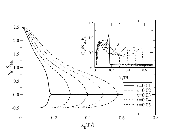
FIG. 1.: The average Mn spin $S_{Mn}$ and the average spin per charge carrier $s_{h}=\sum_{i}s_{h}(i)/N_{h}=s_{hole}/p$ for doping concentrations $x=0.01,0.02,0.03,0.04$ and 0.05, and $p=10\%$. Due to their antiferromagnetic interaction, the two expectation values have opposite sign, with the Mn spin saturating at ${5\over 2}$ and the charge carrier spin saturating at $-{1\over 2}$ at low temperatures. The Mn spin curves have an uncharacteristic shape, with inflection points as explained in the text. In the inset we plot the specific heat per Mn impurity as a function of temperature. The lower peak is due to Mn spin fluctuations, while the upper peak is due to charge carrier fluctuations.

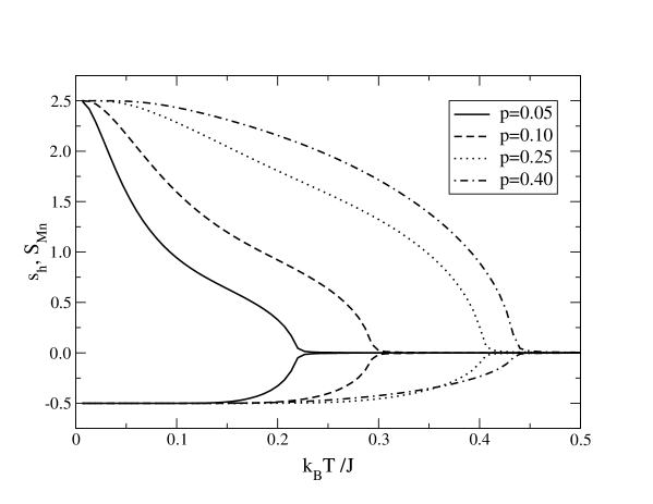
FIG. 2.: Evolution of the average Mn spin $S_{Mn}$ and the average spin per charge carrier $s_{h}$ for different charge carrier concentrations $p=5,10,25$ and $40\%$. The Mn concentration is fixed at $x=0.02$. With large $p$, the shape of $S_{Mn}$ becomes more like the usual convex upward function seen in typical ferromagnets. However, for low doping concentrations $p$ the relatively few charge carriers can only fully magnetize all the Mn spins at very low temperatures.

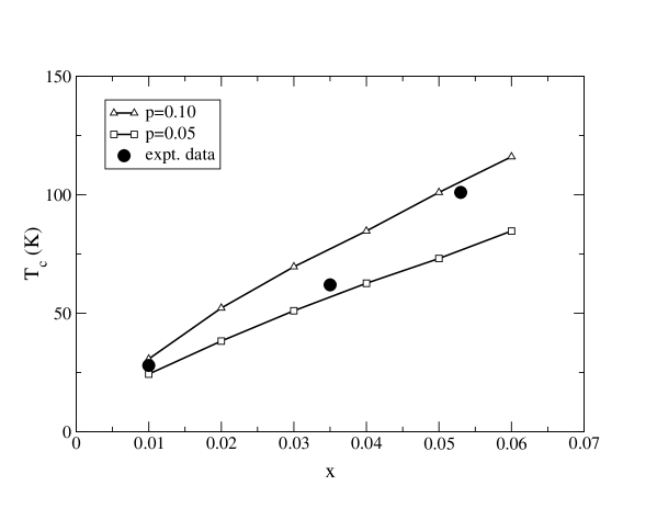
FIG. 3.: Comparison between experimentally measured critical temperatures $T_{c}$ (full circles, from Ref. 10), and values obtained in the mean-field approximation for the ordered Mn spin case. The experimental points fall between the lines corresponding to $p=5\%$ and $p=10\%$, which is the estimated range of charge carrier concentration for these crystals.[10] However, the $T_{c}$ values are very strongly dependent on $p$ (see Fig.2) as well as other parameters of the model.

FIG. 4.: Left panel: Comparison between values for the average Mn spin $S_{Mn}$ and the average charge carrier spin $s_{h}$ obtained with biased initial conditions (full line) and random initial conditions (circles). For random initial conditions we actually plot $|S_{Mn}|>0$ (full circles) and $-|s_{h}|<0$ (empty circles), since the two expectation values always have opposite sign, but the orientation is arbitrary. Results are for $x=0.00926$, $p=10\%$. Right panel: the difference in energy per Mn spin between random and biased initial configurations, as a function of temperature. Full line is $k_{B}T/N_{d}$. For details, see text.

FIG. 5.: (a) Histogram (in arbitrary units) of the total density of charge carriers at each Mn site $\log_{10}(\rho(i))$, for random Mn configuration with $x=0.00926$ and $p=10\%$. The dotted line corresponds to $k_{B}T/J=0.0006$, while the full line corresponds to $k_{B}T/J=0.6$. The vertical line indicates the position of the $\delta$-function that describes the same histogram for an ordered Mn lattice. The two-peaked structure of the histogram for the disordered samples shows that in this case some Mn interact with holes much more strongly than the average, while some Mn spins interact with holes much more weakly than the average. Inset: Same, but for temperatures $k_{B}T/J=0.6$ (full line) and $k_{B}T/J=1.5$ (dotted line). (b) Comparison between the density of charge carrier histogram for $x=0.00926$ (dotted line) and $x=0.05$ (full line) systems. Both systems have $p=10\%$ and $k_{B}T/J=0.0005$. Vertical lines show the corresponding values for the ordered systems. The double-peaked structure is also visible in the higher density sample.

FIG. 6.: The average Mn spin $S_{Mn}$ and average spin per hole $s_{h}$ for doping concentration $x=0.00926$ and $p=10\%$. In increasing order of $T_{c}$, the curves correspond to ordered, weakly disordered, moderately disordered and completely random distributions of Mn (see text).

FIG. 7.: The average Mn spin $S_{Mn}$ and the average spin per hole $s_{h}$ for doping concentration $x=0.05$ and $p=10\%$ (thick lines) and $30\%$ (thin lines) for typical random Mn distributions (full lines) and simple cubic ordered Mn distributions (dashed lines).

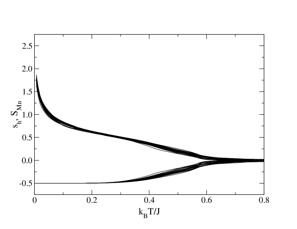
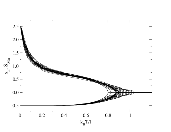
FIG. 8.: Magnetizations for 25 realizations of Mn positional disorder, for $x=0.00926$ (upper panel) and $x=0.05$ (lower panel). The long tails near $T_{c}$ (especially for the lower density) are due to polarization of a few very dense clusters of Mn, and would be destroyed by thermal fluctuations.

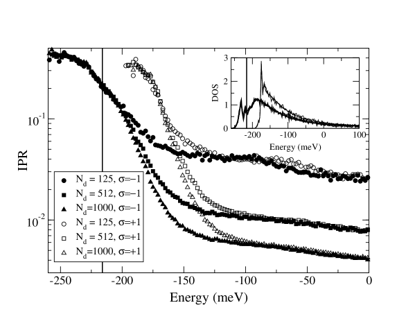
FIG. 9.: Average Inverse Participation Ratio as a function of energy for the $\sigma=\downarrow$ (full symbols) and $\sigma=\uparrow$ (empty symbols) sub-bands of completely random Mn distributions with $p=10\%$, $x=0.00926$ and $N_{d}=125$ (circles), 512 (squares) and 1000 (triangles). The vertical line shows the Fermi energy. Clearly, all the occupied states are localized. In the inset we plot the total Density of States for the two subbands, in arbitrary units.

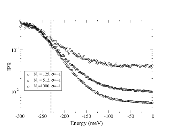
FIG. 10.: Average Inverse Participation Ratio as a function of energy for the $\sigma=\downarrow$ subband of systems with strong disorder (full symbols) and medium-disorder (empty symbols), for $p=10\%$, $x=0.00926$ and $N_{d}=125$ (circles), 512 (squares) and 1000 (triangles). The vertical line shows the Fermi energy of the system with strong disorder (full line) and medium disorder (dashed line). For these parameters, a medium-disordered sample is just above the MIT, while a strongly disordered one is just below the MIT.

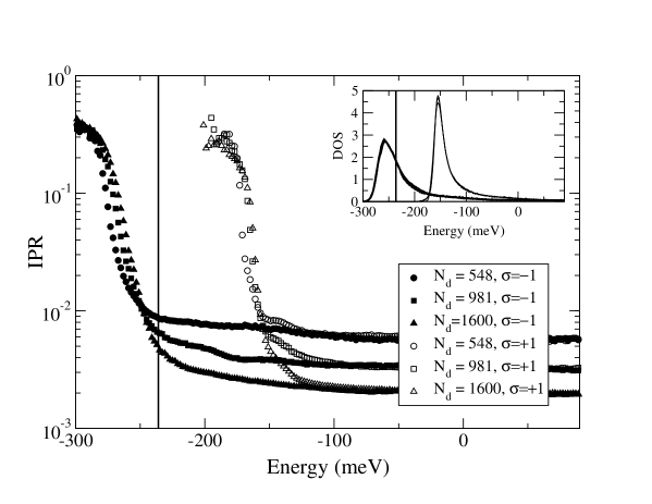
FIG. 11.: Average Inverse Participation Ratio as a function of energy for the $\sigma=\downarrow$ (full symbols) and $\sigma=\uparrow$ (empty symbols) subbands of completely random Mn distributions with $p=10\%$, $x=0.05$ and $N_{d}=548$ (circles), 981 (squares) and 1600 (triangles). The vertical line shows the Fermi energy, above the mobility edge. In the inset we plot the total Density of States for the two subbands, in arbitrary units.

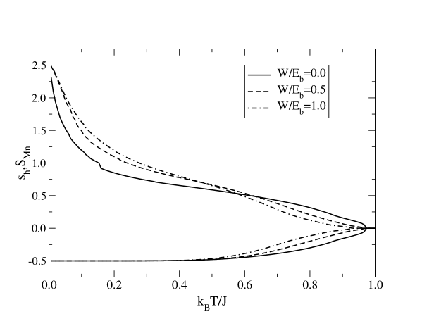
FIG. 12.: Mn spin and charge carrier average magnetization as a function of temperature, for one random Mn configuration corresponding to $x=0.05$ and $p=10\%$, and different values of the on-site disorder cut-off $W/E_{b}=0,0.5$ and 1.While on-site disorder does not affect $T_{c}$ considerably, it does change the shape of the magnetization curves.

FIG. 13.: Comparison between magnetization curves in the absence of an on-site interaction $u(i)=0$ (dashed line), and with an on-site interaction due to As antisites, as explained in text (full line). The curves correspond to the same disordered positions for the Mn sites, and $x=0.00924$ and $p=10\%$.

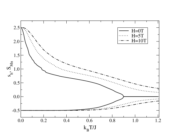
FIG. 14.: Mn spin and charge carrier average magnetization as a function of temperature, for one random Mn configuration corresponding to $x=0.05$ and $p=10\%$, for an external magnetic field $H=0,5$ and 10T. The overall magnetization is significantly increased at lower temperatures, since the external magnetic field polarizes all the Mn spins, not only the ones in the strongly interacting regions.

FIG. 15.: Mn spin and charge carrier average magnetization as a function of $T/T_{c}$, for one random Mn configuration corresponding to $x=0.00926$ and $p=10\%$. The curves correspond to: (a) hopping allowed between all sites, same-sign hopping integral ($T_{c}/J\sim 0.6$); (b) hopping allowed only for sites with $r_{h}=2.22a_{B}$ of each other, same-sign hopping integral ($T_{c}/J\sim 0.2$); (c) hopping allowed between all sites, random-sign hopping integral ($T_{c}/J\sim 0.12$); (d) hopping allowed only for sites with $r_{h}=2.22a_{B}$ of each other, random-sign hopping integral ($T_{c}/J\sim 0.2$). Sample averaging is required to obtain smooth curves. For more details, see text.

FIG. 16.: Effect of an on-site interaction $U$ = 1 Ry (treated within the mean-field approximation) on the magnetization curves corresponding to $x=0.01$ and $p=10\%$ (dashed curve). For comparison, the curves obtained in the absence of an on-site interaction, for the same realization of disorder, are shown as well (full line).

REFERENCES

- [1] for a review of properties of ferromagnetic III-V semiconductors, see H. Ohno, J. Magn. Magn. Mat. 200, 110 (1999).
- [2] H. Ohno, A. Shen, F. Matsukura, A. Oiwa, A. Endo, S. Katsumoto and Y. Iye, Appl. Phys. Lett. 69, 363 (1996).
- [3] T. Hayashi, M. Tanaka, T. Nishinaga, H. Shimada, H. Tsuchiya, Y. Otsuka, J. Cryst. Growth 175, 1063 (1997).
- [4] A. Van Esch, L. Van Bockstal, J. De Boeck, G. Verbanck, A. S. van Steenbergen, P. J. Wellmann, G. Grietens, R. Bogaerts, F. Herlach and G. Borghs, Phys. Rev. B 56, 13103 (1997).
- [5] T. Dietl, A. Haury and Y. M. d’Aubigné, Phys. Rev. B 55, R3347 (1997); M. Takahashi, Phys. Rev. B 56, 7389 (1997); T. Jungwirth, W. A. Atkinson, B. H. Lee and A. H. MacDonald, Phys. Rev. B 59, 9818 (1999); T. Dietl, H. Ohno, F. Matsukura, J. Cibert and D. Ferrand, Science 287, 1019 (2000).
- [6] J. König, H.-H. Lin and A. H. MacDonald, Phys. Rev. Lett. 84, 5628 (2000).
- [7] A. K. Bhattacharjee and C. B. á la Guillaume, Solid State Comm. 113, 17 (2000).
- [8] B. I. Shklovskii and A. L. Efros, Electronic Properties of Doped Semiconductors, (Springer-Verlag, Berlin, 1984).
- [9] R. N. Bhatt and M. T. Rice, Phys. Rev. B 23, 1920 (1981).
- [10] B. Beschoten, P.A. Crowell, I. Malajovich, D. D. Awschalom, F. Matsukura, A. Shen and H. Ohno, Phys. Rev. Lett. 83, 3073 (1999).
- [11] S. Katsumoto, A. Oiwa, Y. Iye, H. Ohno, F. Matsukura, A. Shen, Y. Sugawara, phys. stat. sol. (b) 205, 115 (1998).
- [12] Mona Berciu and R. N. Bhatt, Phys. Rev. Lett. 87, 107203 (2001).
- [13] J. Schliemann, J. Konig and A.H. MacDonald, Phys. Rev. B 64, 165201 (2001).
- [14] R. N. Bhatt, Phys. Rev. B 24, 3630 (1981).
- [15] J. Schliemann and A. H. MacDonald, cond-mat/0107573.
- [16] Malcolm P. Kennett, Mona Berciu and R. N. Bhatt, cond-mat/0102315.
- [17] A. Oiwa, S. Katsumoto, A. Endo, M. Hirasawa, Y. Iye, H. Ohno, F. Matsukura, A. Shen and Y. Sugawara, Solid State Comm. 103, 209 (1997).
- [18] F. Matsukura, H. Ohno, A. Shen and Y. Sugawara, Phys. Rev. B 57, R2037 (1998).
- [19] J. G. E. Harris, D. D. Awschalom, F. Matsukura, H. Ohno, K.D . Maranowski and A. C. Gossard, Appl. Phys. Lett. 75, 1140 (1999).
- [20] A. J. Millis, invited talk at the International Conference on Novel Aspects of Spin-Polarized Transport and Spin Dynamics, Washington DC, Aug. 9-11, 2001.
- [21] A. L. Chudnovskiy, cond-mat/0108396.
- [22] A. Chattopadhyay, S. Das Sarma and A. J. Millis, cond-mat/0106455.
- [23] Uniform magnets as well as metallic alloys are characterized by weak deviations from a universal curve on a versus and plot. [See T. Kaneyoshi, Introduction to Amorphous Magnets, p 56-61 (World Scientific, 1992)].
- [24] Malcolm P. Kennett, Mona Berciu and R. N. Bhatt, unpublished; R. N. Bhatt, X. Wan, M. P. Kennett and M. Berciu, submitted to Comp. Phys. Comm.
- [25] See e.g. S. Oseroff and P. H. Keesom in Diluted Magnetic Semiconductors , edited by J. K. Furdyna and J. Kossut (Academic Press, 1988).
- [26] H. Munekata, H. Ohno, S. von Molnar, A. Segmüller, L. L. Chang and L. Esaki, Phys. Rev. Lett. 63, 1849 (1989).