Multi-patch model for transport properties of cuprate superconductors

Abstract

A number of normal state transport properties of cuprate superconductors are analyzed in detail using the Boltzmann equation. The momentum dependence of the electronic structure and the strong momentum anisotropy of the electronic scattering are included in a phenomenological way via a multi-patch model. The Brillouin zone and the Fermi surface are divided in regions where scattering between the electrons is strong and the Fermi velocity is low (hot patches) and in regions where the scattering is weak and the Fermi velocity is large (cold patches). We present several motivations for this phenomenology starting from various microscopic approaches. A solution of the Boltzmann equation in the case of N patches is obtained and an expression for the distribution function away from equilibrium is given. Within this framework, and limiting our analysis to the two patches case, the temperature dependence of resistivity, thermoelectric power, Hall angle, magnetoresistance and thermal Hall conductivity are studied in a systematic way analyzing the role of the patch geometry and the temperature dependence of the scattering rates. In the case of $Bi$-based cuprates, using ARPES data for the electronic structure, and assuming an inter-patch scattering between hot and cold states with a linear temperature dependence, a reasonable agreement with the available experiments is obtained.
PACS numbers: 72.10.Di, 74.25.Fy, 71.10.Ay

]

I Introduction

The normal state transport properties of cuprate superconductors have attracted enormous attention. In the underdoped regime a pseudogap appears in the excitation spectrum of the metallic state above the superconducting critical temperature $T_{c}$ and below a doping dependent crossover temperature $T^{*}$. At optimum doping the $T^{*}$ almost coincides with $T_{c}$ and the pseudogap region of the phase diagram, if present, is very narrow. On the other hand the metallic state of cuprates at optimum doping, away from the pseudogap region, still strongly deviates from what is observed in simple metals. At optimum doping the in-plane DC-resistivity is linear in temperature from $T_{c}$ to very high temperatures [2, 3], the thermoelectric power is linear [4], the cotangent of the Hall angle displays a $T^{\gamma}$-dependence, ($\gamma\simeq 2$ in $La$-based and $Y$-based cuprates [5, 6], with deviations at low temperature of the order of $2T_{c}$, $1.60\leq\gamma\leq 2$ in $Bi$-based cuprates [7, 8], where increasing the doping decreases the exponent $\gamma$), the magnetoresistance has approximately a $T^{-\alpha}$ dependence, with $\alpha\simeq 4$ [8] and the thermal Hall conductivity has approximately a $T^{-\beta}$ dependence, with $\beta\simeq 1.2$ [9]. Increasing the doping, in the overdoped regime, the conventional Fermi liquid character of the metallic state is almost recovered.

Theoretical approaches to the problem of transport properties of cuprates can be classified in: (i) approaches where in-plane transport properties are analyzed in terms of two scattering times, one associated to the response to an electric field (determining DC-conductivity) and the other one associated to the response to a magnetic field (determining Hall conductivity and magnetoresistance) [11]; (ii) approaches based on the Boltzmann theory [15], where the scattering time is momentum dependent and the Fermi surface can be divided in hot regions (around the $M$ points of the Brillouin zone (BZ)) corresponding to strong scattering between quasiparticles (short scattering time) and low Fermi velocity and cold regions (around the nodal points located along the diagonals $\Gamma Y$ and $\Gamma X$ of the BZ), corresponding to weak scattering (large scattering time) and large Fermi velocity. In the various models [12, 13, 14] proposed within the class (ii), the temperature dependence of the scattering time in the hot regions strongly deviates from the $T^{2}$ behavior of simple metals, while recovering this conventional behavior in the cold regions. Hot/cold regions (or spots) models are able to capture some anomalous properties of cuprates, but a general consensus and a systematic analysis of the full set of electric and thermal transport properties is lacking in the literature.

In this paper we study in a systematic way the normal state transport properties of cuprate superconductors within the second approach. We introduce a new parameterization of the scattering matrix in the Boltzmann equation (BE) for the quasiparticle distribution function via a multi-patch model, motivated by the strong momentum dependence of the electronic properties observed in the cuprates in angle resolved photoemission spectroscopy (ARPES). The BE is solved in the case of N patches and an expression for the perturbed quasiparticle distribution function is obtained. Our analysis is then limited for simplicity to the case of two patches, leaving the multi-patch problem for future investigations. Within the two-patch model the BZ and the Fermi surface (FS) are divided into two regions, the hot regions corresponding to hot patches on the FS and the cold regions corresponding to cold patches on the FS [16]. Assuming a $T^{2}$ temperature dependence for the scattering amplitude in the cold region, a $T$ dependence for the inter-patch (hot-cold) scattering and a constant temperature dependence in the hot region, a reasonable description of the available experimental data for $Bi$-based cuprates is obtained.

ARPES experiments, mainly performed in $Bi2212$ compounds, give a qualitative justification to the division of the BZ and of the FS in cold and hot regions. ARPES clearly shows that the line-shape of the spectral function is strongly momentum dependent [18, 19]. Around the $M$ points of the Brillouin zone $(\pm\pi,0)$; $(0,\pm\pi)$ the spectral function is very broad (the line-width is of the order of $0.2-0.3eV$ at $T=100K$ [19]) and a quasiparticle peak cannot be easily distinguished; the states around the $M$ points are therefore almost incoherent (as localized states) and a very strong scattering mechanism is at the origin of the broad line-shape. Moreover the electronic band dispersion has saddle points located at the $M$ points and this originates the van Hove singularity in the density of states. The band dispersion along the $MY$ direction is very narrow ($\Delta\epsilon\approx 50meV$ for optimally doped $Bi2212$) and the Fermi velocity is low [20]. These states correspond therefore to hot states. The incoherent behavior and the associated line-shape is also temperature independent in the wide range of temperature between $T_{c}$ and $300K$. On the other hand, around the nodal points of the BZ located along the $\Gamma Y(X)$ diagonals, the spectral function has a well pronounced quasiparticle peak (the line-width is of the order of $0.05-0.1eV$ at $T=100K$ [19]) and the wave-vector dispersion of this peak together with the temperature dependence of the peak width can be followed. Valla et al. found a linear temperature and frequency dependence of the peak width for states around the nodal points [21]. Moreover the band dispersion along $\Gamma Y(X)$ is wide ($\Delta\epsilon\approx 400meV$ for optimally doped $Bi2212$) and the Fermi velocity is high. The ratio of the Fermi velocities in the two regions is $v_{F}(\Gamma Y)/v_{F}(M)\simeq 3$ [22]. The quasiparticle states around the nodal points are therefore coherent (delocalized states) and a scattering mechanism with weaker intensity (even with unconventional nature) is at the origin of the line-shape behavior. These states correspond to cold states.

The physics of cuprates is very rich. Starting from the low doping insulating phase, the holes added to the $CuO_{2}$ planes of cuprates through out-of-plane doping will become metallic and segments of a FS appear. The holes move in an antiferromagnetic background and two holes with opposite spins on the same lattice site experience a strong Hubbard repulsion. The conducting holes are therefore strongly correlated and a possible description of the electronic properties of the metallic state of cuprates has been formulated in terms of the two dimensional Hubbard model, eventually with the inclusion of other terms in the Hamiltonian (extended Hubbard model) to take into account short range attraction due to phonons and/or long range Coulomb interaction which can be relevant at high doping. First insights in the phase diagram (temperature vs. doping) of the (extended) Hubbard model indicate the presence of several electronic instabilities arising from the competition between the different degrees of freedom present in the Hamiltonian, such as the kinetic term (delocalizing term) and the short range terms (localizing terms). The most relevant phases, toward which the system is unstable, are the antiferromagnetic insulating phase, phase separation in macroscopic regions with low and high density of holes, spin and charge ordering in the form of stripes, and finally superconductivity. The metallic state of cuprates, in particular in the underdoped region of the phase diagram, can be close to one of these electronic instabilities. Therefore, the properties of the metallic state of cuprates can be strongly connected to the presence of several competing interactions which arise nearby the electronic instabilities mentioned above.

There are two possible microscopic origins for the momentum differentiation of the BZ, one connected to electronic scattering mediated by spin, charge or pair fluctuations and another associated with proximity to a Mott transition.

The first possibility for the momentum differentiation of the BZ is based on its connection to electronic scattering due to spin fluctuations [23]. Superconducting fluctuations [12] and charge instabilities [24] have also been involved. These fluctuations can mediate the electron-electron interaction in both the particle-hole and particle-particle channels and hence they can determine strong deviations in the properties of the metallic state, such as the line-shape of the ARPES spectra and the shape of the FS respect to a conventional Fermi liquid picture. The various fluctuations have a specific momentum and frequency dependence and the propagators are peaked at different critical momenta $\mathbf{q}_{c}$, depending from the underlying instability: for phase separation $\mathbf{q}_{c}=0$ [24], for antiferromagnetic insulator $\mathbf{q}_{c}=\mathbf{Q}\equiv(\pi,\pi)$ [33], for charge ordering $\mathbf{q}_{c}=\mathbf{q}_{stripe}$ [34, 35], where $q_{stripe}=2\pi/\lambda_{stripe}$ ($\lambda_{stripe}$ is the periodicity of the charge modulation). Therefore, the critical fluctuations couple electrons with momenta only inside particular segments of FS, and the specific geometry of the strongly coupled (and hence of the weakly coupled) segments is determined by the interplay between the shape of the FS and $\mathbf{q}_{c}$. This leads to the phenomenology of the two- or multi-patch model for the electronic scattering in the metallic state of cuprates.

The second scenario for momentum differentiation invokes the proximity to a Mott transition. It builds on our recent understanding of this phenomena within dynamical mean field theory (DMFT) [25] and its extension: the two impurity method [25, 26], the Bethe-Peierls cluster [25], the dynamical cluster approximation (DCA) [27, 28, 29] and the cellular dynamical mean field theory (C-DMFT) [30, 31, 36].

DMFT allows a microscopic description of the strongly correlated state near the Mott transition. There is a temperature scale reminiscent of the Kondo temperature $T_{K}$, such that for $T\ll T_{K}$ the quasiparticles are Fermi liquid like, while for $T>T_{K}$ the single particle excitations become incoherent and the transport properties are non Fermi liquid like. In single site DMFT studies, the two regimes were obtained by varying the temperature and the strength of the local Hubbard repulsion $U$, and by construction they occur uniformly in the BZ. Relaxing the constraint of momentum independent selfenergy by using the C-DMFT, one envisions that different patches of BZ have different Kondo temperatures, leading naturally to the multi-patch model presented here. According to this view, therefore, the microscopic origin of the multi-patch division of the BZ and of the FS of cuprate superconductors can be associated to the presence of a nearby transition from a (non conventional) metallic state to a Mott antiferromagnetic insulator. A detailed microscopic derivation of the many-patch model is in progress, using the C-DMFT.

These views on momentum space differentiation may be complementary, and there are already strong hints from numerical calculations by Onoda and Imada [37], that they occur in the Hubbard model.

The plan of the paper is the following. In Section II we recall the BE in the linearized form and we introduce the multi-patch model for the the scattering operator. The scattering operator of the BE is projected on the patches and temperature dependences of its coefficients are assigned. A set of smooth functions is introduced to permit a continuous transition between hot and cold regions. A solution of the BE in the case of N patches is given in terms of the perturbed quasiparticle distribution function. In Section III the results for the normal state transport properties obtained by the two-patch model are presented in a systematic way. The temperature dependences of resistivity, thermoelectric power, cotangent of the Hall angle, magnetoresistance and thermal Hall conductivity are reported. The various transport properties are studied for different set of parameters and the relevant hot/cold patch is associated to every quantity. Our model is applied to the normal state transport properties of $Bi$-based cuprates ($Bi2212$ and $Bi2201$) and, taking ARPES data as input for the electronic structure, we find a reasonable agreement with the available experimental data. Discussions and conclusions are given in Section IV.

II The Boltzmann equation and the multi-patch model

ARPES experiments show that optimally and overdoped cuprates have a large FS in the normal state and well defined quasiparticles exist in a sizeable (cold) region of the BZ around the $\Gamma Y(X)$ directions. The existence of a FS and quasiparticles makes the treatment within the framework of the BE possible. We start our analysis introducing the linearized BE. As we are interested in electrical, heat and Hall transport properties, we consider three terms in the BE, the terms including the electric field $\mathbf{E}$ and the temperature gradient $\nabla_{\mathbf{r}}T/T$ (driving terms) and the term including the magnetic field $\mathbf{B}$ (bending term). We consider here uniform electric and magnetic field. In this case the linearized BE has the following form:

$$\frac{\partial}{\partial t}g_{\mathbf{k}} + \left(-\frac{\partial f_{\mathbf{k}}^{0}}{\partial\epsilon_{\mathbf{k}}}\right)\epsilon_{\mathbf{k}}{\mathbf{v}}_{\mathbf{k}}\cdot\frac{\nabla_{\mathbf{r}}T}{T}$$ (1)

$$+ e{\mathbf{E}}{\mathbf{v}}_{\mathbf{k}}\left(\frac{\partial f_{\mathbf{k}}^{0}}{\partial\epsilon_{\mathbf{k}}}\right)+\frac{e}{\hbar c}[{\mathbf{v}}_{\mathbf{k}}\times{\mathbf{B}}]\cdot\frac{\partial\tilde{g}_{\mathbf{k}}}{\partial\mathbf{k}}=C_{\mathbf{k}}$$ (2)

where $\tilde{g}_{\mathbf{k}}=g_{\mathbf{k}}+(-\partial f_{\mathbf{k}}^{0})/(\partial\epsilon_{\mathbf{k}})\sum_{\mathbf{k}^{\prime}}f_{\mathbf{k},\mathbf{k}^{\prime}}g_{\mathbf{k}^{\prime}}$ takes the interaction between quasiparticles $f_{\mathbf{k},\mathbf{k}^{\prime}}$ into account (Fermi liquid corrections) [38] and $g_{\mathbf{k}}$ is the departure from the equilibrium distribution function $f_{\mathbf{k}}^{0}$. ${\mathbf{v}_{\mathbf{k}}}$ is the group velocity of the quasiparticles. The scattering operator $C_{\mathbf{k}}$ has the form $C_{\mathbf{k}}=\sum_{\mathbf{k}^{\prime}}\left[C_{\mathbf{k},\mathbf{k}^{\prime}}\tilde{g}_{\mathbf{k}^{\prime}}-C_{\mathbf{k},\mathbf{k}^{\prime}}\tilde{g}_{\mathbf{k}}\right]$, where $C_{\mathbf{k},\mathbf{k}^{\prime}}$ is the scattering matrix, describing the scattering of quasiparticles on an effective bosonic mode or impurity centers with the first term describing scattering ”in” to the state $\mathbf{k}$ and the second term describing scattering ”out” of the state $\mathbf{k}$. The relaxation time $\tau_{\mathbf{k}}$ for the state $\mathbf{k}$ is defined as $1/\tau_{\mathbf{k}}\equiv\sum_{\mathbf{k}^{\prime}}C_{\mathbf{k},\mathbf{k}^{\prime}}$. Within the conventional microscopic approach to the transport properties of a Fermi liquid, the transport equation for the distribution function can be written in terms of the four-point vertex part $\Gamma({\mathbf{k},\mathbf{k}^{\prime},\mathbf{q},\omega})$ [32]. The scattering matrix $C_{\mathbf{k},\mathbf{k}^{\prime}}$ is then identified with the $\mathbf{q}=0$, $\omega=0$ limit of the irreducible part of the vertex $C_{\mathbf{k},\mathbf{k}^{\prime}}=$i$(z^{2}/2)\Gamma^{(1)}({\mathbf{k},\mathbf{k}^{\prime},\mathbf{q}=0},\omega=0)$, where $z^{2}$ is the mass renormalization and $\Gamma^{(1)}$ is the irreducible vertex. Below we will use this identification to give a first microscopic justification to our choice of $C_{\mathbf{k},\mathbf{k}^{\prime}}$. In the steady-state case we can replace $\tilde{g}_{\mathbf{k}}\rightarrow g_{\mathbf{k}}$ as every term in Eq. (1) is expressed in terms of $\tilde{g}_{\mathbf{k}}$. Therefore the knowledge of the form of $f_{\mathbf{k},\mathbf{k}^{\prime}}$ is not required in the steady-state case. Frequency-dependent transport processes require both $\tilde{g}_{\mathbf{k}}$ and $g_{\mathbf{k}}$, and hence the knowledge of $f_{\mathbf{k},\mathbf{k}^{\prime}}$ becomes important. In the steady-state case the number of quasiparticles $g_{\mathbf{k}}$ contributing to transport is given by

$$\left[\frac{e}{\hbar c}({\mathbf{v}}_{\mathbf{k}}\times\mathbf{B})\cdot\nabla_{\mathbf{k}}\right. + \left.\frac{1}{\tau_{\mathbf{k}}}\right]g_{\mathbf{k}}-\sum_{\mathbf{k}^{\prime}}C_{\mathbf{k},\mathbf{k}^{\prime}}g_{\mathbf{k}^{\prime}}=$$ (3)

$$= \left[e{\mathbf{v}}_{\mathbf{k}}\cdot{\mathbf{E}}-\epsilon_{\mathbf{k}}{\mathbf{v}}_{\mathbf{k}}\cdot\frac{\nabla_{\mathbf{r}}T}{T}\right]\left(-\frac{\partial f_{\mathbf{k}}^{0}}{\partial\epsilon_{\mathbf{k}}}\right).$$ (4)

Defining the operator $\hat{A}_{\mathbf{k},\mathbf{k}^{\prime}}$ as

$$\hat{A}_{\mathbf{k},\mathbf{k}^{\prime}}\equiv\left[\frac{1}{\tau_{\mathbf{k}}}+\frac{e}{\hbar c}(\mathbf{v}_{\mathbf{k}}\times\mathbf{B})\cdot\nabla_{\mathbf{k}}\right]\delta_{\mathbf{k},\mathbf{k}^{\prime}}-C_{\mathbf{k},\mathbf{k}^{\prime}}$$ (5)

allows us to write the l.h.s. of Eq. (3) in the form $\sum_{\mathbf{k}^{\prime}}\hat{A}_{\mathbf{k},\mathbf{k}^{\prime}}g_{\mathbf{k}^{\prime}}$ and hence the inverse of $\hat{A}_{\mathbf{k},\mathbf{k}^{\prime}}$ is required to solve Eq. (3). Considering weak magnetic fields, the bending term containing the magnetic field in the BE can be treated as a small perturbation of the transport process. We split $\hat{A}_{\mathbf{k},\mathbf{k}^{\prime}}$ in two parts, $\hat{A}_{\mathbf{k},\mathbf{k}^{\prime}}=\hat{K}_{\mathbf{k},\mathbf{k}^{\prime}}+\hat{M}_{\mathbf{k},\mathbf{k}^{\prime}}^{B}$, with a magnetic field independent part $\hat{K}_{\mathbf{k},\mathbf{k}^{\prime}}=(1/\tau_{\mathbf{k}})\delta_{\mathbf{k},\mathbf{k}^{\prime}}-C_{\mathbf{k},\mathbf{k}^{\prime}}$ and a part that contains the magnetic field $\hat{M}_{\mathbf{k},\mathbf{k}^{\prime}}^{B}=\left[(e/\hbar c)(\mathbf{v}_{\mathbf{k}}\times\mathbf{B})\cdot\nabla_{\mathbf{k}}\right]\delta_{\mathbf{k},\mathbf{k}^{\prime}}$. A perturbative expansion of $\hat{A}_{\mathbf{k},\mathbf{k}^{\prime}}$ in powers of $\mathbf{B}$ allows us to write the inverse of this operator as

$$\hat{A}_{\mathbf{k},\mathbf{k}^{\prime}}^{-1} = \hat{K}_{\mathbf{k},\mathbf{k}^{\prime}}^{-1}-\hat{K}_{\mathbf{k},\mathbf{k}^{i}}^{-1}\hat{M}_{\mathbf{k}^{i},\mathbf{k}^{j}}^{B}\hat{K}_{\mathbf{k}^{j},\mathbf{k}^{\prime}}^{-1}$$ (6)

$$+ \hat{K}_{\mathbf{k},\mathbf{k}^{i}}^{-1}\hat{M}_{\mathbf{k}^{i},\mathbf{k}^{j}}^{B}\hat{K}_{\mathbf{k}^{j},\mathbf{k}^{k}}^{-1}\hat{M}_{\mathbf{k}^{k},\mathbf{k}^{l}}^{B}\hat{K}_{\mathbf{k}^{l},\mathbf{k}^{\prime}}^{-1}+{\mathcal{O}}(B^{3})$$ (7)

with a summation over repeated indexes. Depending on the quantity of interest, we get contribution from the different terms in this expansion. The first term gives the leading order contribution to the DC and thermal conductivity, the second term to the (thermal) Hall-conductivity and the third term to the magnetoresistance. It follows from Eq. (3) that the number of particles $g_{\mathbf{k}}$ contributing to transport is given by

$$g_{\mathbf{k}}=\sum_{\mathbf{k}^{\prime}}\hat{A}^{-1}_{\mathbf{k},\mathbf{k}^{\prime}}\left[e{\mathbf{v}_{\mathbf{k}^{\prime}}}\cdot{\mathbf{E}}-\epsilon_{\mathbf{k}^{\prime}}{\mathbf{v}_{\mathbf{k}^{\prime}}}\cdot\frac{\nabla_{\mathbf{r}}T}{T}\right]\left(-\frac{\partial f_{\mathbf{k}^{\prime}}^{0}}{\partial\epsilon_{\mathbf{k}^{\prime}}}\right).$$ (8)

This equation is the starting point of our analysis. Electrical and thermal conductivities are derived using $g_{\mathbf{k}}$ obtained from Eq. (8).

The transport properties are separable in electric and thermal properties. All possible currents are given by

$$\left(\begin{array}[]{c}\mathbf{j}_{e}\\ \mathbf{j}_{Q}\end{array}\right)=\left(\begin{array}[]{cl}\bar{\sigma}&\bar{S}\\ \bar{S}&\bar{\kappa}\end{array}\right)\left(\begin{array}[]{c}\mathbf{E}\\ -\frac{\nabla T}{T}\end{array}\right)$$ (9)

where ${\mathbf{j}}_{e}$ is the electric current, $\mathbf{j}_{Q}$ is the thermal current, $\bar{\sigma}$ is the electrical conductivity tensor, $\bar{\kappa}$ is the thermal conductivity tensor and $\bar{S}$ is the thermopower tensor. Note that Eq. (9) contains a symmetric matrix using $\nabla T/T$ as driving term for thermal gradients. The currents defined in Eq. (9) can also be expressed in terms of quasiparticles. The electric and the thermal currents are given by ${\mathbf{j}}_{e}=e\sum_{\mathbf{k}}{\mathbf{v}}_{\mathbf{k}}g_{\mathbf{k}}$ and ${\mathbf{j}}_{Q}=\sum_{\mathbf{k}}{\mathbf{v}}_{\mathbf{k}}\epsilon_{\mathbf{k}}g_{\mathbf{k}}$. (When frequency dependence is considered, $g_{\mathbf{k}}$ has to be replaced with $\tilde{g}_{\mathbf{k}}$ in the expression of the currents given above.) The tensors defined in Eq. (9) are given by:

$$\sigma^{\mu\nu}=2e^{2}\sum_{\mathbf{k},\mathbf{k}^{\prime}}v^{\mu}_{\mathbf{k}}\hat{A}^{-1}_{\mathbf{k},\mathbf{k}^{\prime}}v^{\nu}_{\mathbf{k}^{\prime}}\left(-\frac{\partial f_{\mathbf{k}^{\prime}}^{0}}{\partial\epsilon_{\mathbf{k}^{\prime}}}\right)$$ (10)

$$\kappa^{\mu\nu}=2\sum_{\mathbf{k},\mathbf{k}^{\prime}}v^{\mu}_{\mathbf{k}}\epsilon_{\mathbf{k}}\hat{A}^{-1}_{\mathbf{k},\mathbf{k}^{\prime}}\epsilon_{\mathbf{k}^{\prime}}v^{\nu}_{\mathbf{k}^{\prime}}\left(-\frac{\partial f_{\mathbf{k}^{\prime}}^{0}}{\partial\epsilon_{\mathbf{k}^{\prime}}}\right)$$ (11)

$$S^{\mu\nu}=-2e\sum_{\mathbf{k},\mathbf{k}^{\prime}}v^{\mu}_{\mathbf{k}}\epsilon_{\mathbf{k}}\hat{A}^{-1}_{\mathbf{k},\mathbf{k}^{\prime}}v^{\nu}_{\mathbf{k}^{\prime}}\left(-\frac{\partial f_{\mathbf{k}^{\prime}}^{0}}{\partial\epsilon_{\mathbf{k}^{\prime}}}\right)$$ (12)

with the inverse of the operator $\hat{A}_{\mathbf{k},\mathbf{k}^{\prime}}$ given in Eq. (6). The factor $2$ in the expressions above takes the spin degeneracy into account.

The last unknown quantity in Eq. (3) is the scattering matrix $C_{\mathbf{k},\mathbf{k}^{\prime}}$. The scattering matrix is connected via a frequency integration to the spectral function of the effective bosonic mode exchanged in the electronic scattering. As discussed above, ARPES suggests that the bosonic mode is strongly momentum dependent and divides the BZ in hot and cold regions. In order to include in the scattering matrix a non trivial momentum dependence and the cold/hot division of the BZ, while maintaining a simple solution of the BE, a possibility is to expand $C_{\mathbf{k},\mathbf{k}^{\prime}}$ with respect to a basis of functions which are able to select the various regions of the BZ, according to the momentum dependence of the effective bosonic mode. Therefore, the scattering matrix $C_{\mathbf{k},\mathbf{k}^{\prime}}$ can be written as

$$C_{\mathbf{k},\mathbf{k}^{\prime}}=\sum_{i,j=1}^{N}a_{ij}\Phi_{i}({\mathbf{k}})\Phi_{j}({\mathbf{k}^{\prime}}),$$ (13)

where $\Phi_{i}(\mathbf{k})$ is a function which is equal to one inside the $i$-th patch of the BZ and zero outside, and it interpolates continuously between these two values; $a_{ij}$ is the amplitude of the scattering between the $i$-th and the $j$-th region of the BZ, it is in general temperature dependent and $((a_{ij}))$ is a symmetric matrix with real elements; N is the total number of regions of the BZ required to include properly the main effects of the anisotropy of the scattering and its interplay with the shape of the FS.

One possible microscopic motivation for the form of the scattering matrix given in Eq. (13) is based on the connection between $C_{\mathbf{k},\mathbf{k}^{\prime}}$ and the four-point vertex $\Gamma$ discussed above Eq. (3) and on the C-DMFT. The four-point vertex can in principle be evaluated by C-DMFT and the general structure of the irreducible vertex will be $\Gamma^{(1)}({\mathbf{k}},{\mathbf{k}^{\prime}},{\mathbf{q}},\omega)=\sum_{\alpha,\beta,\gamma,\delta}\Gamma^{c}_{\alpha,\beta,\gamma,\delta}(\omega)\phi_{\alpha}^{{\dagger}}({\mathbf{k}})\phi_{\beta}({\mathbf{k}^{\prime}})\phi_{\gamma}^{{\dagger}}({\mathbf{k}+\mathbf{q}})\phi_{\delta}({\mathbf{k}^{\prime}+\mathbf{q}})$. Once the patch function is defined as $\Phi_{i=(\alpha,\beta)}({\mathbf{k}})=\phi_{\alpha}^{{\dagger}}({\mathbf{k}})\phi_{\beta}({\mathbf{k}})$, Eq. (13) for $C_{\mathbf{k},\mathbf{k}^{\prime}}$ can be recovered. The coefficient $a_{ij}$ entering Eq. (13) are then defined in terms of the four-point vertex of the cluster as $a_{i=(\alpha,\beta),j=(\gamma,\delta)}=$i$(z^{2}/2)\Gamma^{c}_{\alpha,\beta,\gamma,\delta}(\omega=0)$.

The form of the scattering matrix given in Eq. (13) permits an analytical solution of the linearized BE for $g_{\mathbf{k}}$ defined above. Considering the electric field and the thermal gradient as external perturbations, Eq. (3) gives

$$g_{\mathbf{k}}=\tau_{\mathbf{k}}\left[e{\mathbf{v_{k}}}{\mathbf{E}}-\epsilon_{{\mathbf{k}}}{\mathbf{v_{k}}}\frac{\nabla_{{\mathbf{r}}}T}{T}\right]\left(-\frac{\partial f_{{\mathbf{k}}}^{0}}{\partial\epsilon_{{\mathbf{k}}}}\right)+\tau_{{\mathbf{k}}}\sum_{i,j=1}^{N}a_{ij}\Phi_{i}({\mathbf{k}})\cdot$$ (14)

$$\cdot\sum_{\mathbf{k^{\prime}}}\left[e{\mathbf{v_{k}}}{\mathbf{E}}-\epsilon_{{\mathbf{k}}}{\mathbf{v_{k}}}\frac{\nabla_{{\mathbf{r}}}T}{T}\right]\left(-\frac{\partial f_{\mathbf{k^{\prime}}}^{0}}{\partial\epsilon_{\mathbf{k^{\prime}}}}\right)\sum_{l=1}^{N}T^{-1}_{jl}\Phi_{l}({\mathbf{k^{\prime}}}),$$ (15)

which reduces the solution of the BE to a matrix inversion problem for the N² elements of a matrix $T_{jl}$ given by

$$T_{jl}=\delta_{jl}-\sum_{m=1}^{N}a_{mj}\sum_{\mathbf{k}}\Phi_{m}({\mathbf{k}})\tau_{\mathbf{k}}\Phi_{l}({\mathbf{k}}).$$ (16)

From Eq. (14) and Eq. (16) we can obtain the inverse of the matrix $\hat{K}_{\mathbf{k},\mathbf{k}^{\prime}}$, defined above Eq. (6), as follow

$$\hat{K}^{-1}_{\mathbf{k},\mathbf{k}^{\prime}}=\tau_{\mathbf{k}}\delta_{\mathbf{k},\mathbf{k}^{\prime}}+\tau_{\mathbf{k}}\tau_{\mathbf{k^{\prime}}}\sum_{i,j=1}^{N}a_{ij}\Phi_{i}({\mathbf{k}})\sum_{l=1}^{N}T^{-1}_{jl}\Phi_{l}({\mathbf{k^{\prime}}}).$$ (17)

Once we know the explicit expression for the operator $\hat{K}^{-1}_{\mathbf{k},\mathbf{k}^{\prime}}$, we are able to evaluate the expansion of the operator $\hat{A}^{-1}_{\mathbf{k},\mathbf{k}^{\prime}}$ for weak magnetic fields given in Eq. (6). Inserting the operator $\hat{A}^{-1}_{\mathbf{k},\mathbf{k}^{\prime}}$ in Eq. (8), we can evaluate the solution of the linearized BE, given by $g_{\mathbf{k}}$, in the presence of an electric field, a thermal gradient and a weak magnetic field. $g_{\mathbf{k}}$ can be then used to evaluate all the currents given above Eq. (10). All the response functions given in Eqs. (10, 11, 12) are obtained inserting directly the expression for $\hat{A}^{-1}_{\mathbf{k},\mathbf{k}^{\prime}}$.

In the following we consider a minimal realization of this multi-patch approximation limiting our analysis to N=2 patches. The two-patch model permits the distinction between cold and hot regions on the BZ and the FS and it is suitable to describe the main properties of the scattering between electrons and an effective mode peaked at large momenta ($e.g.$ an antiferromagnetic spin fluctuation peaked at $\mathbf{Q}\equiv(\pi;\pi)$). On the other hand, to include the effect of the (small momenta) forward scattering, important for transport mainly in the cold region, a larger number of patches is required (at least N=5), and we deserve this case for further investigation.

In the case N=2, the two-patch division of the BZ and of the Fermi surface is realized by introducing two functions $\Phi_{\mathbf{k}}$ and $\Psi_{\mathbf{k}}$: $\Phi_{\mathbf{k}}$ describes the cold region and $\Psi_{\mathbf{k}}$ the hot region as indicated in Fig. 1.

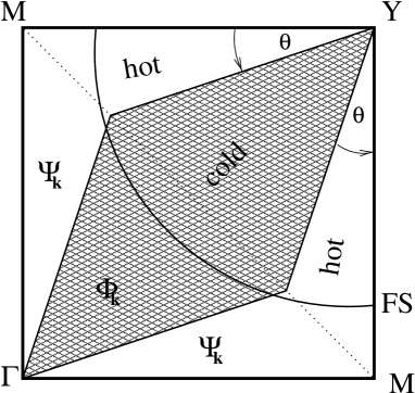
FIG. 1.: The first quadrant of the BZ is splitted into cold and hot regions. Cold regions are described by a function $\Phi_{\mathbf{k}}$ and hot regions by a function $\Psi_{\mathbf{k}}$. The angle $\theta$ parameterizes the size of the hot regions.

The cold region is described by four boundaries as shown in Fig. 1. The angle $\theta$, defined with respect to the $Y=(\pi,\pi)$ point of the BZ, parameterizes the size of the hot regions (and hence of the cold regions). The reason to split the whole BZ (and not only the FS) into a cold and a hot part is that the term $\partial f^{0}/\partial\epsilon$ in Eq. (3) doesn’t restrict the sum over $\mathbf{k}$ on the FS any more when we increase size-ably the temperature, studying $T$-dependent properties. As the leading contribution to the magnetoresistance is given by the third term in Eq. (6), which contains two derivatives with respect to $k_{x},k_{y}$ (given by $\hat{M}^{B}$ repeated two times), the magnetoresistance diverges in the case of a discontinuous change between the two patches. Therefore we introduce functions $\Phi_{\mathbf{k}}$ and $\Psi_{\mathbf{k}}$ varying smoothly between the two regions. We use hyperbolic tangents to describe the smooth change between the two regions and a parameter $w$ is introduced to describe the width of the transition region. In the limit $w\rightarrow 0$ a step function is recovered, $\theta(x)=\lim_{w\rightarrow 0}(1+\tanh(x/w))/2$. Finally, we define two slopes, $m_{1}$ and $m_{2}$, and two offsets, $t_{1}$ and $t_{2}$, given by $m_{1}=\cot(\theta)>0$, $m_{2}=\tan(\theta)>0,m_{1}>m_{2}$, $t_{1}=\pi(1-\tan(\theta))>0$ and $t_{2}=\pi(1-\cot(\theta))<0$. In the case of smooth functions, the cold region in the first quadrant of the BZ (see Fig. 1) is described by:

$$\Phi_{\mathbf{k}}=\prod_{i=1}^{4}\Phi_{i}({\mathbf{k}})$$ (18)

with

$$\Phi_{1}({\mathbf{k}}) = \frac{1}{2}\left[1-\tanh\left(\frac{k_{y}-m_{1}k_{x}}{w}\right)\right];$$

$$\Phi_{2}({\mathbf{k}}) = \frac{1}{2}\left[\tanh\left(\frac{k_{y}-m_{2}k_{x}}{w}\right)+1\right];$$

$$\Phi_{3}({\mathbf{k}}) = \frac{1}{2}\left[1-\tanh\left(\frac{k_{y}-m_{2}k_{x}-t_{1}}{w}\right)\right];$$

$$\Phi_{4}({\mathbf{k}}) = \frac{1}{2}\left[\tanh\left(\frac{k_{y}-m_{1}k_{x}-t_{2}}{w}\right)+1\right].$$

The smooth change between the two patches is shown in Fig. 2.

FIG. 2.: Smooth change between the two patches. The parameter $w$ describes the width of the transition region between the two patches and it allows to study the effects of this region on transport properties.

The hot region is described by $\Psi_{\mathbf{k}}=1-\Phi_{\mathbf{k}}$. Note that $\Psi_{\mathbf{k}}$ vanishes only asymptotically in the cold region and vice versa.

Following the phenomenological approach described above, the scattering matrix can be written consisting of different scattering mechanisms in different patches. In the case of the two-patch model, we introduce three parameters that describe the possible scattering, scattering inside the cold or inside the hot region and scattering between the two (hot/cold) regions,

$$C_{\mathbf{k},\mathbf{k}^{\prime}}=a\Phi_{\mathbf{k}}\Phi_{\mathbf{k}^{\prime}}+b\Psi_{\mathbf{k}}\Psi_{\mathbf{k}^{\prime}}+c[\Phi_{\mathbf{k}}\Psi_{\mathbf{k}^{\prime}}+\Psi_{\mathbf{k}}\Phi_{\mathbf{k}^{\prime}}].$$ (19)

The scattering matrix $C_{\mathbf{k},\mathbf{k}^{\prime}}$ given in Eq. (19) is written as a sum of terms which have a separate dependence from $\mathbf{k}$ and ${\mathbf{k}}^{\prime}$. This approximation permits an analytic solution of the BE for $g_{\mathbf{k}}$, while having a non trivial momentum dependence and symmetry properties of the scattering process. With the symmetric scattering matrix given in Eq. (19), we obtain a momentum dependent relaxation time $\tau_{\mathbf{k}}$, $1/\tau_{\mathbf{k}}\equiv\sum_{\mathbf{k}^{\prime}}C_{\mathbf{k},\mathbf{k}^{\prime}}$,

$$\tau_{\mathbf{k}}=\frac{1}{C_{\Phi}\Phi_{\mathbf{k}}+C_{\Psi}\Psi_{\mathbf{k}}}$$ (20)

with $C_{\Phi}=\alpha a+(1-\alpha)c$ and $C_{\Psi}=(1-\alpha)b+\alpha c$, where, in the limit $w\rightarrow 0$, $\alpha$ describes the area of the cold region, $\alpha=\sum_{\mathbf{k}}\Phi_{\mathbf{k}}$, and $1-\alpha$ the area of the hot region, $1-\alpha=\sum_{\mathbf{k}}\Psi_{\mathbf{k}}$. All the sums are normalized with respect to the number of $k$-points of the BZ. In the limit $w\rightarrow 0$ we get two different lifetimes in the cold and in the hot regions:

$$\lim_{w\rightarrow 0}\tau_{\mathbf{k}}=\left\{\begin{array}[]{ll}\tau_{c}=\frac{1}{\alpha a+(1-\alpha)c}&\mbox{in cold regions},\\ \tau_{h}=\frac{1}{\alpha c+(1-\alpha)b}&\mbox{in hot regions}.\end{array}\right.$$ (21)

We consider the following temperature dependences of the scattering amplitudes in the scattering matrix:

$$a(T)=\bar{a}T^{2};\;b(T)=\bar{b};\;c(T)=\bar{c}T,$$ (22)

with the temperature independent parameters $\bar{a}$, $\bar{b}$ and $\bar{c}$ having proper dimensions given by $\left[\hbar\bar{a}/k_{B}^{2}\right]=1/eV$, $\left[\hbar\bar{b}\right]=eV$ and $\left[\hbar\bar{c}/k_{B}\right]=1$. Indeed, in the cold region the scattering is weak and a Fermi liquid behavior with a $T^{2}$ temperature dependence of the scattering matrix $C_{\mathbf{k},\mathbf{k}^{\prime}}$ (with both $\mathbf{k},\mathbf{k}^{\prime}$ inside the cold region) is a reasonable assumption. On the other hand, in the hot region the scattering is strong and, as suggested by ARPES, the states are almost incoherent; we consider $C_{\mathbf{k},\mathbf{k}^{\prime}}$ (with both $\mathbf{k},\mathbf{k}^{\prime}$ inside the hot region) as temperature independent. Finally, we introduce a coupling between the hot and cold regions. The inter-patches elements of $C_{\mathbf{k},\mathbf{k}^{\prime}}$ (with $\mathbf{k}$ inside the cold region and $\mathbf{k}^{\prime}$ inside the hot region and vice-versa) are considered to be temperature dependent with a linear in $T$ dependence, and this is a key assumption in our model to obtain the linear temperature dependence of the resistivity, as shown in the next section. The important consequence of our assumptions for $C_{\mathbf{k},\mathbf{k}^{\prime}}$, and in particular the introduction of the inter-patches scattering with a linear temperature dependence, is that at low temperature the scattering amplitude is non-Fermi liquid at any ${\bf k}$-point of the BZ. Indeed in the cold region we have $1/\tau_{c}=\alpha\bar{a}T^{2}+(1-\alpha)\bar{c}T$, while in the hot region $1/\tau_{h}=(1-\alpha)\bar{b}+\alpha\bar{c}T$. The Fermi liquid behavior can be recovered in the cold region when the area of the hot region tends to zero (i.e. $\alpha=1$). The non Fermi liquid behavior of the scattering amplitude in the cold region at low temperature is supported by the ARPES experiments of Valla et al. [21], as already discussed.

To solve the BE, it is necessary to find how the operator $\hat{K}^{-1}$ acts on an arbitrary velocity, as can be seen in Eq. (8). Because of the symmetry properties of the scattering matrix $C_{\mathbf{k},\mathbf{k}^{\prime}}$ and of the quasiparticle velocity $\mathbf{v_{k}}$, when summing over the whole BZ, $\sum_{\mathbf{k}^{\prime}}C_{\mathbf{k},\mathbf{k}^{\prime}}{\mathbf{v}_{\mathbf{k}^{\prime}}}=0$ [40]. Using these properties, we find that $\hat{K}^{-1}$ acts on an arbitrary velocity just by inserting a scattering time $\tau_{\mathbf{k}}$, that is momentum dependent, in front of the velocity, $\sum_{\mathbf{k}^{\prime}}\hat{K}_{\mathbf{k},\mathbf{k}^{\prime}}^{-1}v_{\mathbf{k}^{\prime}}^{\nu}=\tau_{\mathbf{k}}v_{\mathbf{k}}^{\nu}$. This allows us to solve exactly the linearized BE and to obtain formulas for the several transport properties we are interested in. The deviation $g_{\mathbf{k}}$ from the equilibrium distribution function $f_{\mathbf{k}}^{0}$ is $g_{\mathbf{k}}=eE\tau_{\mathbf{k}}{\mathbf{v}_{\mathbf{k}}}\cdot{\hat{{\bf n}}}(-\partial f_{\mathbf{k}}^{0}/\partial\epsilon_{\mathbf{k}})$, where ${\hat{{\bf n}}}$ is the direction of the external electric field ${\mathbf{E}}=E{\hat{{\bf n}}}$. The momentum dependence of $g_{\mathbf{k}}$ is therefore given by $g_{\mathbf{k}}\sim{\mathbf{v}_{\mathbf{k}}}\cdot{\hat{{\bf n}}}/(C_{\Phi}\Phi_{\mathbf{k}}+C_{\Psi}\Psi_{\mathbf{k}})$ and hence in the hot regions $g_{\mathbf{k}}$ is strongly suppressed while in the cold regions $g_{\mathbf{k}}$ has sizeable values. Hlubina and Rice, solving the BE by a variational approach in the case of hot spots generated by antiferromagnetic fluctuations coupled to fermions, obtained a $g_{\mathbf{k}}$ with similar properties, i.e. a depopulation of the hot regions [14] (see Section IV for a discussion). Finally, as regard the single particle electronic properties, we recall that optimally and overdoped cuprates display very similar shape and momentum dependence of the Fermi surface and of the electronic band dispersion. Therefore we consider $Bi2212$ as typical for the FS and band structure of cuprates. For this material several ARPES measurements are available. We consider a tight-binding model for the band structure of $Bi2212$ with hopping up to the fifth nearest neighbors. We are using the following fit for the energy of the quasiparticles $\epsilon(\mathbf{k})$ obtained by Norman et al. [39].

$$\epsilon(k_{x},k_{y})=\sum_{i=1}^{6}c_{i}\eta_{i}(k_{x},k_{y})$$ (23)

with the values of the coefficients $c_{i}$ and the functions $\eta_{i}$ given by $c_{1}=0.1305eV$, $c_{2}=-0.5951eV$, $c_{3}=0.1636eV$, $c_{4}=-0.0519eV$, $c_{5}=-0.1117eV$, $c_{6}=0.0510eV$ and $\eta_{1}=1$, $\eta_{2}=0.5[\cos(k_{x})+\cos(k_{y})]$, $\eta_{3}=\cos(k_{x})\cos(k_{y})$, $\eta_{4}=0.5[\cos(2k_{x})+\cos(2k_{y})]$, $\eta_{5}=0.5[\cos(2k_{x})\cos(k_{y})+\cos(2k_{y})\cos(k_{x})]$, $\eta_{6}=\cos(2k_{x})\cos(2k_{y})$. These parameters are appropriate for the band structure of $Bi2212$ compounds at optimum doping, thus giving an open FS and a van Hove singularity (VHS) slightly below the Fermi level. The value of $\epsilon_{F}=-c_{1}=-0.1305eV$ is fixed to have the proper distance of the Fermi level from the VHS ($\epsilon_{F}-\epsilon_{VHS}=35meV$ as determined experimentally), and corresponds to the optimum doping $\delta=0.17$. The bandwidth of the dispersion given in Eq. (23) is $1.4eV$.

III Transport properties

A Resistivity

Theoretical results. The leading order contribution to the DC-conductivity is given by the first term in Eq. (6), thus $\hat{A}^{-1}_{\mathbf{k},\mathbf{k}^{\prime}}$ is replaced by $\hat{K}^{-1}_{\mathbf{k},\mathbf{k}^{\prime}}$ and inserted into Eq. (10). The operator $\hat{K}^{-1}_{\mathbf{k},\mathbf{k}^{\prime}}$, applied on a velocity $v_{\mathbf{k}}$ gives $v_{\mathbf{k}}\tau_{\mathbf{k}}$, as already discussed in Section II. Therefore, the DC-conductivity is given by:

$$\sigma^{xx}=2e^{2}\sum_{\mathbf{k}}\left(-\frac{\partial f_{\mathbf{k}}^{0}}{\partial\epsilon_{\mathbf{k}}}\right)(v_{\mathbf{k}}^{x})^{2}\tau_{\mathbf{k}}.$$ (24)

In the limit $T\rightarrow 0$ we can obtain a finite contribution to $\sigma^{xx}$ depending on the width $w$ and on the angle $\theta$ (determining the area of the hot region). As $\tau_{\mathbf{k}}$ given in Eq. (20) doesn’t diverge in the case $w\neq 0$ (because $\Psi_{\mathbf{k}}\neq 0$ even inside the cold region), we get a finite contribution to $\sigma^{xx}$ and a residual resistivity at zero temperature. Note that the residual resistivity is determined by the width $w$ and $\bar{b}(1-\alpha)$, thus the $T$-independent part in the coefficient $C_{\Psi}$. In the limit $w\rightarrow 0$ we separate two regions in the BZ and we can consider a hot and a cold average velocity, $v_{h}$ and $v_{c}$ respectively. In the limit of low $T$ and $w\rightarrow 0$, the DC-conductivity is given by

$$\lim_{w\rightarrow 0}\sigma^{xx}=e^{2}\left[v_{c}^{2}\tau_{c}N_{c}(\epsilon_{F})+v_{h}^{2}\tau_{h}N_{h}(\epsilon_{F})\right].$$ (25)

The quantity $N_{c}(\epsilon_{F})$ is the density of states at the Fermi level in the cold region, $N_{c}(\epsilon)=\sum_{\mathbf{k}}\delta(\epsilon_{\mathbf{k}}-\epsilon)\Phi_{\mathbf{k}}$, while $N_{h}(\epsilon_{F})$ is the same quantity in the hot region, with $N_{h}(\epsilon)=\sum_{\mathbf{k}}\delta(\epsilon_{\mathbf{k}}-\epsilon)\Psi_{\mathbf{k}}$. Fig. 3 shows the density of states in the hot (upper panel) and in the cold region (lower panel) as a function of the size of the hot region (determined by the angle $\theta$) in the limit $w\rightarrow 0$, obtained using the band dispersion given in Eq. (23). Eq. (25) shows that cold and hot regions are wired in parallel, while each region (cold/hot) is wired in series with the transition region (in the case $w=0$), as shown by the structure of $\tau_{c}$ and $\tau_{h}$ given in Eq. (21). In the limits mentioned above the temperature dependence of the resistivity up to second order in $T$ is given by:

$$\lim_{w\rightarrow 0}\rho^{xx} = \frac{1}{e^{2}}\frac{(1-\alpha)\bar{c}}{v_{c}^{2}N_{c}(\epsilon_{F})}T$$ (27)

$$\left[1+\left(\frac{\alpha}{1-\alpha}\frac{\bar{a}}{\bar{c}}-\frac{\bar{c}}{\bar{b}}\left(\frac{v_{h}}{v_{c}}\right)^{2}\frac{N_{h}(\epsilon_{F})}{N_{c}(\epsilon_{F})}\right)T\right].$$

As both lifetimes $\tau_{c}$ and $\tau_{h}$ for $w=0$ diverge in the limit $T\rightarrow 0$, the resistivity has no zero temperature offset, $\rho(T\rightarrow 0)=0$. However an offset can be obtained by a finite width $w$ as discussed above.

FIG. 3.: The overall shape of the hot density of states $N_{h}(\epsilon)$ (upper panel), doesn’t change with $\theta$, while the magnitude at the Fermi level changes. In the case of the cold density of states $N_{c}(\epsilon_{F})$ (lower panel), both the overall shape and the magnitude at the Fermi level changes. The position of the Fermi level $E_{F}$, corresponding to optimum doping, is also reported. Note the changement of sign in the derivative of $N_{c}(\epsilon_{F})$ for $\theta=12.9^{\circ}$.

In our two-patch model we can associate the doping variation of the electronic properties of the cuprates mainly with the variation of the area of the hot region and hence with the angle $\theta$. Indeed, ARPES experiments on $Bi2212$ show that the region of the BZ where the spectral function is broad and no quasiparticle peaks are detectable increases as the doping is reduced. A small segment of (quasiparticle) FS is observed approaching the metal-insulator transition [10]. Therefore, we can translate this behavior of the FS and of the spectral function saying that when the doping is decreased, the angle $\theta$ increases (i.e., the size of the hot region increases). Fig. 4 shows the change in resistivity with increasing angle $\theta$; we obtain that the residual resistivity increases with increasing angle $\theta$.

FIG. 4.: Resistivity $\rho(T)$ for different sizes of the hot region (i.e. different $\theta$) as a function of temperature. The variation of the hot region changes the offset of the resistivity. It can be seen that increasing the area of the hot region increases the residual resistivity $\rho_{0}$ and change slightly the power law behavior $\rho(T)\sim T^{\gamma}$. The following parameters are used: ${\bar{a}}=48$, ${\bar{b}}=2$, ${\bar{c}}=7$ and $w=0.3$. $\theta$ changes between $10^{\circ}$ and $30^{\circ}$.

As can be seen in Eq. (27) the hot/cold scattering term $\bar{c}$ is the most important quantity in determining the slope of the resistivity respect to the other scattering amplitude $\bar{a}$ and $\bar{b}$. The variation of the slope with $\bar{c}$ is reported in Fig. 5. Note that a variation in $\bar{c}$ doesn’t change the residual resistivity.

FIG. 5.: The amplitude of the scattering between the cold and the hot region, described by $\bar{c}$, determines the slope of the resistivity. Note that $\rho_{0}$ doesn’t change. Increasing the inter-patch scattering determines an increasing in the slope of the DC-resistivity. The following parameters are used: $\bar{a}=48$, $\bar{b}=2$, $\theta=20^{\circ}$ and $w=0.3$. $\bar{c}$ changes between $5$ and $9$.

Moreover, the slope of the resistivity is controlled by the single particle properties of the cold region, in particular by the cold density of states $N_{c}(\epsilon_{F})$ and by the Fermi velocity $v_{c}^{2}$, and by the area of the cold region $\alpha$, as obtained in Eq. (27).

On the other hand, the influence of the prefactor $(1-\alpha)/(v_{c}^{2}N_{c}(\epsilon_{F}))$ on the slope of the resistivity is small in comparison with the influence of $\bar{c}$, as can be seen in Fig. 4 and Fig. 5, because of compensation effects: $v_{c}N_{c}(\epsilon_{F})$ is roughly $\theta$ independent and also the ratio $(1-\alpha)/v_{c}$ is expected to vary smoothly with $\theta$.

Comparison with experiments. The linearity of the resistivity up to very high temperatures was found experimentally (see, e.g. [8]). Experiments show a quasi-linear temperature dependence of the resistivity $\rho^{xx}(T)\propto T^{\gamma}$, where in Ref. [8] it is shown that $\gamma$ increases with doping. For optimally doped systems $\gamma=1$, while for overdoped systems a $\gamma>1$ ($\gamma\simeq 1.5$) is observed, supporting a gradual recovering of the Fermi liquid properties. The doping dependence of the exponent $\gamma$ can be compared with our results in Fig. 4, showing that small values of $\theta$ ($\theta<15^{\circ}$) give a resistivity $\rho(T)\sim T^{\gamma}$ with $\gamma>1$. Moreover the residual resistivity $\rho_{0}=\rho(T=0)$ increases with underdoping and this is in agreement with the trend obtained in Fig. 4. Therefore, the two-patch model provides the possibility to change the doping mainly by changing the angle $\theta$, besides considering the doping dependence of $\epsilon_{F}$ and $v_{F}({\mathbf{k}})$. Note that the range of the change in $\rho$ with changing doping is observed in Ref. [8] as well. Fig. $1$ of Ref. [8] shows that for underdoped $Bi2201$ (with a $La$ concentration of $x=0.66$) the offset $\rho_{0}\simeq 150\mu\Omega cm$, while for the overdoped compound (with $x=0.24$) $\rho_{0}\simeq 40\mu\Omega cm$. The increase in the slope and in the offset of the resistivity is also observed in $Y123$ as the doping is reduced [42]: the offset changes between $250\mu\Omega cm$ and $20\mu\Omega cm$ (Fig. 1(a) of Ref. [42]). The same range of variation is given in our results of Fig. 4 considering the range $10^{\circ}<\theta<25^{\circ}$. Within the described change in $\theta$ a big variation of doping can be described.

In the following paragraph we report a simple explicit comparison between the transport properties here evaluated and the experimental data via a fitting procedure. The comparison here presented is limited to the $Bi$-based cuprates ($Bi2212$ and $Bi2201$) for which several ARPES and transport experimental data are available.

The strategy of fitting the experimental data is the following. We introduce a temperature scale $T_{0}$ upon which the term linear in $T$ in the scattering rate in the cold region dominates. This guarantees us that the resistivity is linear up to this temperature $T_{0}$. We choose a temperature $T_{0}$ that has a value of $\approx 1000K$. The relations $\bar{a}=(1-\alpha)\bar{c}/(\alpha T_{0})$ and $\bar{b}=\alpha\bar{c}T_{0}/(1-\alpha)$ allows us to obtain first values of $\bar{a}$ and $\bar{b}$ for given $T_{0}$ and $\bar{c}$. The width of the transition region $w$ is fixed mainly by the magnetoresistance as shown in section III-D. Starting with different angles $\theta$ (i.e. different sizes of the hot region), we try to get a good fit of Hall-angle data as shown in section III-C. Then we try to fit the Hall-angle and the slope of the resistivity for different combination of $\theta$ and $\bar{c}$. It turns out that the angle $\theta\approx 20^{\circ}$ and the value $\bar{c}\approx 6.5$ gives a good fit of the Hall-angle and of the slope of the resistivity. After that, we change the scattering amplitude $\bar{b}$ in the hot region. Increasing $\bar{b}$ leads to an higher resistivity and thus the parameter $\bar{b}$ allows us to adjust the offset of the resistivity. In this manner we can fix the parameters $w,\theta,\bar{c},\bar{b}$. The last parameter that is to be fixed is $\bar{a}$. The freedom for the parameter $\bar{a}$ is not big, in order to maintain the linearity of the resistivity. Thus the initial condition we have chosen for $\bar{a}$ can remain valid. We obtain a reasonable fit for the different transport quantities with the following values of the parameters: $w=0.20$, $\bar{a}=60$, $\bar{b}=2.1$, $\bar{c}=7.0$ and $\theta=20^{\circ}$. In Fig.6 we report the resistivity as a function of temperature evaluated by Eq. (24) with the set of parameters given above and we compare our results with the resistivity measured in $Bi2212$ at optimum doping as given in Ref. [2] and in Ref. [44].

FIG. 6.: Fit of the temperature dependence of the resistivity for the set of parameters given in the text. The experimental data are from an optimally doped $Bi2212$ samples from Ref. [1] and from Ref. [43].

B Thermoelectric power

Theoretical results. To evaluate the thermoelectricpower (TEP), which is the quantity measured in experiments, we first compute the longitudinal thermopower $S^{xx}$ given in Eq. (12). The thermopower has almost the same expression as the DC-conductivity besides the extra factor of $\epsilon_{\mathbf{k}}$ and an extra minus in the sum, and it is given by

$$S^{xx}=-2e\sum_{\mathbf{k}}\left(-\frac{\partial f_{\mathbf{k}}^{0}}{\partial\epsilon_{\mathbf{k}}}\right)\epsilon({\mathbf{k}})(v_{\mathbf{k}}^{x})^{2}\tau_{\mathbf{k}}.$$ (28)

A Sommerfeld-expansion of Eq. (28), in the limit of $w=0$ and at low temperature, gives

$$\lim_{w\rightarrow 0}S^{xx}=-e\frac{\pi^{2}}{3}(k_{B}T)^{2}\left[v_{c}^{2}\tau_{c}N^{\prime}_{c}(\epsilon_{F})+v_{h}^{2}\tau_{h}N^{\prime}_{h}(\epsilon_{F})\right]$$ (29)

with the first derivatives of the density of states $N^{\prime}_{c,h}(\epsilon_{F})$ evaluated at the Fermi level in the cold and in the hot regions. We found that $S^{xx}$ has a smooth dependence on $w$ and hence the limit mentioned above is valid also for small values of the width $w$. As in the case of conductivity, because $\tau_{c}>>\tau_{h}$ and $v_{c}>>v_{h}$, the main contribution to the thermopower comes from the cold region. It is interesting that the Fermi level is below the peak in the cold density of states for $\theta>10^{\circ}$ (see Fig. 3 (lower panel)). The peak in $N_{c}(\epsilon)$ is exactly at the Fermi level for $\theta\approx 10^{\circ}$. The TEP, as measured in the experiments mentioned above, is defined as

$$TEP=\frac{S^{xx}}{T\sigma^{xx}},$$ (30)

where $\sigma^{xx}$ is given in Eq. (24). Again the cold region has the main influence. The expression of the TEP in the limit of $w=0$ and at low temperatures is given by

$$TEP = -\frac{\pi^{2}}{3e}k_{B}^{2}T\frac{N^{\prime}_{c}(\epsilon_{F})+[(v_{h}^{2}\tau_{h})/(v_{c}^{2}\tau_{c})]N^{\prime}_{h}(\epsilon_{F})}{N_{c}(\epsilon_{F})+[(v_{h}^{2}\tau_{h})/(v_{c}^{2}\tau_{c})]N_{h}(\epsilon_{F})}$$ (32)

$$\approx-\frac{\pi^{2}}{3e}k_{B}^{2}T\frac{N^{\prime}_{c}(\epsilon_{F})}{N_{c}(\epsilon_{F})},$$

where the last relation is obtained in the limit $\tau_{c}>>\tau_{h}$ and $v_{c}>>v_{h}$. Therefore the ratio between the derivative of the density of states and the density of states evaluated at the Fermi level in the cold region is the main quantity that determines the slope of the TEP at low temperature. Increasing the temperature above $200K$, we have verified that the contribution of the hot region to the TEP becomes comparable to the contribution from the cold one.

FIG. 7.: Temperature dependence of the thermoelectric power for different angles $\theta$. The following parameters are used: $\bar{a}=48$, $\bar{b}=2$, $\bar{c}=7$ and $w=0.3$. $\theta$ changes between $10^{\circ}$ and $30^{\circ}$.

Note that in the case of the TEP the offset doesn’t change varying $w$. We found that the TEP is the most sensitive quantity to a variation of the electronic structure, in agreement with Ref. [4]. This is done by changing the hopping parameters $c_{1}$ and $c_{2}$ in Eq. (23). Fig. 7 shows the TEP obtained from the two-patch model for different angles $\theta$. For $\theta\geq 10^{\circ}$ the TEP is negative and the slope of the TEP at low temperature changes slightly with different angles $\theta>10^{\circ}$. We found that, as predicted in the limit given in Eq. (32), the TEP is almost not affected by other parameters than $\theta$. Nonetheless we got the largest effect on it from the scattering in the hot region. Again the slope doesn’t change so much and the offset changes also slightly when the hot-scattering $\bar{b}$ is changed of a factor 5, as shown in Fig. 8.

FIG. 8.: Scattering in the hot region slightly affect the slope of the TEP and it has a weak influence on its offset. An increase in the hot-region scattering lowers the TEP and makes it even more negative. The following parameters are used: $\bar{a}=48$, $\bar{c}=7$, $\theta=20^{\circ}$ and $w=0.3$. $\bar{b}$ changes between $0.5$ and $2.5$.

Comparison with experiments. In Fig.9 we report the TEP evaluated by Eq. (28) with the same set of parameters used for the resistivity ($w=0.20$, $\bar{a}=60$, $\bar{b}=2.1$, $\bar{c}=7.0$, $\theta=20^{\circ}$) and we compare our results with the TEP measured in $Bi2201$ at optimum and over doping as given in Ref. [4] and with the TEP measured in $Bi2212$ at optimum and overdoping as given in Ref.[47]. The TEP obtained with our two-patch model is only in qualitative agreement with the TEP observed by experiments. In particular only the overdoped $Bi2201$ has a TEP with a temperature dependence close to the one evaluated within the two-patch model. Note also that the TEP measured in overdoped $Tl2201$ cuprates has almost the same temperature dependence and magnitude of overdoped $Bi2201$ (and hence close to the TEP of the two-patch model), as shown in Fig. 1 of Ref.[47].

FIG. 9.: Comparison between the TEP evaluated by the two-patch model and the thermoelectric data given by McIntosh et al. in Ref. [3] (material: $Bi2201$ at optimum doping (x=0.44) and overdoping (x=0.2)) and by Obertelli et al. in Ref. [46]. (material: $Bi2212$ at optimum doping ($\delta=0.0$) and overdoping ($\delta=0.077$)).

We attribute the quantitative discrepancy between the TEP measured in optimally and underdoped cuprates to the fact that the TEP reflects the properties of the excitations away from the FS and hence the frequency dependence of the scattering amplitude becomes important, as shown by DMFT studies [41]. We deserve the inclusion of the frequency dependence of the scattering amplitudes for future investigation.

C Hall angle

Theoretical results. The leading order contribution to the Hall-conductivity $\sigma^{xy}$ is given by the second term in the expansion of the operator $\hat{A}^{-1}$ respect to the (weak) magnetic field, $\hat{A}^{-1}=-\hat{K}^{-1}\hat{M}_{B}\hat{K}^{-1}$. Inserting this term into Eq. (10), we get the Hall-conductivity $\sigma^{xy}$. The bending term in $\hat{A}^{-1}$ is

$$({\mathbf{v}}_{\mathbf{k}}\times{\mathbf{B}})\nabla_{\mathbf{k}}=B(v_{\mathbf{k}}^{y}\partial_{k_{x}}-v_{\mathbf{k}}^{x}\partial_{k_{y}}),$$ (33)

that arises from the operator $\hat{M}_{B}$ considering a magnetic field perpendicular to the $CuO_{2}$ planes. In this case, the formula for the Hall-conductivity is the following

$$\sigma^{xy}=-2\frac{e^{3}B}{\hbar c}\sum_{\mathbf{k}}\tau_{\mathbf{k}}v_{\mathbf{k}}^{x}\left[v_{\mathbf{k}}^{y}\partial_{k_{x}}-v_{\mathbf{k}}^{x}\partial_{k_{y}}\right]\tau_{\mathbf{k}}v_{\mathbf{k}}^{y}\left(-\frac{\partial f_{\mathbf{k}}}{\partial\epsilon_{\mathbf{k}}}\right).$$ (34)

The partial derivatives of the relaxation time $\tau_{\mathbf{k}}$ enter in Eq. (34) and are given by $\partial\tau_{\mathbf{k}}/\partial k_{x}=-\tau_{\mathbf{k}}^{2}(\partial\Phi_{\mathbf{k}})/(\partial k_{x})\left[C_{\Phi}-C_{\Psi}\right]$ and $\partial\tau_{\mathbf{k}}/\partial k_{y}=-\tau_{\mathbf{k}}^{2}(\partial\Phi_{\mathbf{k}})/(\partial k_{y})\left[C_{\Phi}-C_{\Psi}\right]$ respectively (note that $\partial\Phi_{\mathbf{k}}/\partial k_{x}=-\partial\Psi_{\mathbf{k}}/\partial k_{x}$). The final expression for the Hall-conductivity is

$$\sigma^{xy} = -\frac{2e^{3}B}{\hbar c}\sum_{\mathbf{k}}\left(-\frac{\partial f_{\mathbf{k}}}{\partial\epsilon_{\mathbf{k}}}\right)\tau_{\mathbf{k}}^{2}v_{\mathbf{k}}^{x}\left[v_{\mathbf{k}}^{y}\frac{\partial v_{\mathbf{k}}^{y}}{\partial k_{x}}-v_{\mathbf{k}}^{x}\frac{\partial v_{\mathbf{k}}^{y}}{\partial k_{y}}\right]$$ (35)

$$+ \frac{2e^{3}B}{\hbar c}\sum_{\mathbf{k}}\left(-\frac{\partial f_{\mathbf{k}}}{\partial\epsilon_{\mathbf{k}}}\right)\tau_{\mathbf{k}}^{3}v_{\mathbf{k}}^{x}(v_{\mathbf{k}}^{y})^{2}\frac{\partial\Phi_{\mathbf{k}}}{\partial k_{x}}\left[C_{\Phi}-C_{\Psi}\right]$$ (36)

$$- \frac{2e^{3}B}{\hbar c}\sum_{\mathbf{k}}\left(-\frac{\partial f_{\mathbf{k}}}{\partial\epsilon_{\mathbf{k}}}\right)\tau_{\mathbf{k}}^{3}(v_{\mathbf{k}}^{x})^{2}v_{\mathbf{k}}^{y}\frac{\partial\Phi_{\mathbf{k}}}{\partial k_{y}}\left[C_{\Phi}-C_{\Psi}\right].$$ (37)

This expression contains two different powers of the scattering time, one $\propto\tau_{\mathbf{k}}^{2}$ and another $\propto\tau_{\mathbf{k}}^{3}$. In the limit $w\rightarrow 0$ we can get some further insight in the problem of the Hall-conductivity. In the low temperature limit the sum over $\mathbf{k}$ is restricted on the FS. The Hall-conductivity contains in this limit derivatives of step functions and hence $\delta$-functions are generated. As a consequence we get $8$ points on the FS that contribute to the second and third term in Eq. (35). The temperature dependence of the relaxation time $\tau_{0}$ evaluated in the transition region hot/cold on the FS can be written, using in this region $\Phi_{\mathbf{k}}=\Psi_{\mathbf{k}}=1/2$ and using Eq. (20), as $\tau_{0}=1/(2C_{\Phi}+2C_{\Psi})=1/(\bar{c}_{0}+\bar{c}_{1}T+\bar{c}_{2}T^{2})$. In this limit Eq. (35) can be written in a more compact form as

$$\lim_{w\rightarrow 0}\sigma^{xy} = \sigma_{1}^{xy}+\frac{2e^{3}B}{\hbar c}4\tau_{0}^{3}\left[C_{\Phi}-C_{\Psi}\right]$$

$$\left\{v_{y}(A)v_{y}(B)\left[v_{y}(B)-v_{y}(A)\right]\right\}[q-1]$$

where $\sigma_{1}^{xy}$ is the first term in Eq. (35), $A$ and $B$ label the contributing points on the FS in the first quadrant of the BZ and $q$ is either $\tan\theta$ or $\cot\theta$ depending on $\theta$ respect to the value $\theta\simeq 10^{\circ}$. Note that we get an offset to $\sigma^{xy}$ from the last terms even in the limit $w\rightarrow 0$. Increasing $w$, also the first term in (35) contributes to the offset due to the same reasons given for the resistivity. The first term in (35) contains the customer contribution proportional to $\tau_{\mathbf{k}}^{2}$ while the second term contains higher powers in $\tau_{\mathbf{k}}$ and can originate deviations from the $\tau_{\mathbf{k}}^{2}$ behavior depending from the temperature and the scattering amplitudes.

The cotangent of the Hall-angle is defined as the ratio between the direct conductivity and the Hall conductivity,

$$\cot\theta_{H}(T)=\frac{\sigma^{xx}}{\sigma^{xy}}.$$ (38)

A plot of $\cot\theta_{H}$ vs. $T^{2}$ (see Fig.10) shows that the cotangent of the Hall-angle has a temperature dependence $\propto T^{2}$ in the high temperature regime ($T>200K$), where we observe almost a straight line.

FIG. 10.: The size of the hot region determines the offset of the Hall-angle. In the case of $\theta=30^{\circ}$, which is equivalent to $3/4$ of the first BZ with hot character, the offset in the Hall angle is close to $50$. Note that we plot $\cot\theta_{H}$ vs. $T^{2}$. The following parameters are used $\bar{a}=48$, $\bar{b}=2$, $\bar{c}=7$ and $w=0.3$. $\theta$ changes between $10^{\circ}$ and $30^{\circ}$. The magnetic field is $B=1T$.

It can also be seen in Fig. 10 that the range of temperature where $\cot\theta_{H}\sim T^{2}$ increases with decreasing $\theta$ (i.e. increasing doping). Konstantinovic et al. [7] pointed out the strong influence of the anisotropy of the FS on the Hall-angle. We reproduced this observation by changing the hopping parameters $c_{1}$ and $c_{2}$ in Eq. (23) but we found that the effect of this change has even bigger effects on the TEP, as already discussed. Among the other parameters we found the strongest influence on $\cot\theta_{H}(T)$ from the inter-patch scattering amplitude $\bar{c}$. The effect of $\bar{c}$ on the Hall-angle is shown in Fig. 11.

FIG. 11.: Effect of the hot/cold inter-patch scattering on the Hall-angle. It turns out that $\bar{c}$ has an effect on the temperature dependence of the Hall-angle, but no significant effect on the offset of the Hall-angle contrary to $\theta$. The following parameters are used: $\bar{a}=48$, $\bar{b}=2$, $\theta=20^{\circ}$ and $w=0.3$. $\bar{c}$ changes between 5 and 9. The magnetic field is $B=1T$.

It can be seen that this parameter changes the temperature range where $\cot\theta_{H}\sim T^{2}$ only slightly and the offset is independent on $\bar{c}$. The larger the value of $\bar{c}$ is the smaller the deviation of the Hall-angle from a straight line is, which means that increasing the cold/hot scattering has opposite effect as decreasing the angle $\theta$. On the other hand changing $\theta$ (i.e. doping) effects the offset of the Hall-angle. In the framework of the two-patch model we obtain a decreasing offset of the cotangent of the Hall-angle with increasing doping and an increasing value of the power law coefficient $\gamma$ ($\cot\theta_{H}\propto T^{\gamma}$) with increasing doping.

Comparison with experiments. As already discussed, the range of temperature where $\cot\theta_{H}\sim T^{2}$ increases with decreasing $\theta$ (i.e. increasing doping) (see Fig. 10), which is contrary to the results given in [7] and [8], but in agreement with the results of Ref. [42]. Indeed a careful examination of various set of experimental data for $\cot\theta_{H}$ vs. $T^{2}$ indicates that the exact $T^{2}$ dependence does not extend over the whole temperature range, and deviations are observed for $T<300K$. As shown in Ref. [42], e.g., in $Y123$ as $T_{c}$ is lowered by underdoping, the range of the $T^{2}$ dependence of $\cot\theta_{H}$ moves toward higher temperatures (for $T_{c}=90K$, the deviation start at $T=100K$, while for $T_{c}=40K$, the deviation start at $T=170K$). On the other hand changing $\theta$ (i.e. doping) effects the offset of the Hall-angle which was found in [8]. Indeed in Fig. 3(b) of Ref. [8] the change in the offset of the cotangent of the Hall angle between underdoped (x=0.66) and overdoped (x=0.24) $Bi2201$ compounds measured at $T\simeq 280K$ ($T^{2}\simeq 8\cdot 10^{4}K^{2}$) is of the order of 1300, a value which is compatible with our finding of Fig. 10 ($\simeq 2000$) considering again $10^{\circ}<\theta<25^{\circ}$ as in the case of the resistivity discussed in Section III-A. In the case of $Y123$ the slope of $\cot\theta_{H}$ vs. $T^{2}$ increases when the doping is reduced (almost $30\%$ of variation, when $T_{c}$ is reduced from $90K$ for optimally doped to $40K$ for an underdoped $Y123$, while in this case the offset increases only slightly (see Fig. 1(e), Fig. 3 and Fig. 4 of Ref. [42]). Note that for $Y123$ a non monotonic behavior of the slope of $\cot\theta_{H}$ vs. $T^{2}$ as a function of doping is observed in a different set of measurements reported in Ref. [43]. This can be understood remembering that we increase the hot region increasing $\theta$ (i.e. decreasing doping). In the framework of the two-patch model we obtain a decreasing offset of the cotangent of the Hall-angle with increasing doping and an increasing value of the power law coefficient $\gamma$ ($\cot\theta_{H}\propto T^{\gamma}$) with increasing doping.

In Fig.12 we report the cotangent of the Hall angle evaluated by Eq. (38) with the same set of parameters used for the resistivity and the TEP ($w=0.20$, $\bar{a}=60$, $\bar{b}=2.1$, $\bar{c}=7.0$, $\theta=20^{\circ}$) and we compare our results with the cotangent of the Hall angle measured in $Bi2212$ at optimum doping as given in Ref. [7] and in $Bi2201$ again at optimum doping as given in Ref. [8]. The agreement with the data obtained in $Bi2212$ is good and also a qualitative agreement is obtained if we compare the results obtained with the two-patch model and the band structure of $Bi2212$ with the experimental data for $Bi2201$ at optimum doping.

FIG. 12.: Comparison between the experimental data for the Hall angle and the Hall angle obtained from our two-patch model using the set of parameters given in the text. The experimental data that are shown in the plot correspond to $Bi2212$ at optimum doping from Ref. [6] and to $Bi2201$ at optimum doping from Ref. [7].

D Magnetoresistance

Theoretical results. The magnetoresistance (MR) is defined as the ratio of the variation in the resistivity in presence of a magnetic field to the resistivity without magnetic field. In the transverse geometry, with the magnetic field applied perpendicular to the $CuO_{2}$ planes and the current measured parallel to the planes, the MR is given by

$$MR=\frac{\Delta\rho^{xx}(B)}{\rho^{xx}(0)}\approx-\frac{\Delta\sigma^{xx}(B)}{\sigma^{xx}(0)}-\tan^{2}\theta_{H}.$$ (39)

In this geometry, the first extra contribution to the DC-conductivity, $\Delta\sigma^{xx}(B)$ is achieved by the third term in Eq. (6), thus we have to insert $\hat{A}^{-1}=\hat{K}^{-1}\hat{M}_{B}\hat{K}^{-1}\hat{M}_{B}\hat{K}^{-1}$ into Eq. (10). We get an expression for the correction to the conductivity given by

$$\Delta\sigma^{xx}(B) = 2e^{2}\sum_{\mathbf{k},\mathbf{k}^{1},\mathbf{k}^{2},\mathbf{k}^{3},\mathbf{k}^{4},\mathbf{k}^{5}}v_{\mathbf{k}}^{x}\hat{K}^{-1}_{\mathbf{k},\mathbf{k}^{1}}\hat{M}_{\mathbf{k}^{1},\mathbf{k}^{2}}\hat{K}^{-1}_{\mathbf{k}^{2},\mathbf{k}^{3}}$$ (41)

$$\hat{M}_{\mathbf{k}^{3},\mathbf{k}^{4}}\hat{K}^{-1}_{\mathbf{k}^{4},\mathbf{k}^{5}}v_{\mathbf{k}^{5}}^{x}\left(-\frac{\partial f}{\partial\epsilon_{\mathbf{k}^{5}}}\right).$$

In this case it is necessary to consider partial derivatives of $\tau_{\mathbf{k}}^{2}$ with respect to $k_{x}$ or $k_{y}$, which are given by $\partial\tau^{2}_{\mathbf{k}}/\partial k_{x}=-2\tau_{\mathbf{k}}^{3}\partial\Phi_{\mathbf{k}}/\partial k_{x}\left[C_{\Phi}-C_{\Psi}\right]$ and $\partial\tau^{3}_{\mathbf{k}}/\partial k_{x}=-3\tau_{\mathbf{k}}^{4}(\partial\Phi_{\mathbf{k}})/(\partial k_{x})\left[C_{\Phi}-C_{\Psi}\right]$. Finally we obtain $\Delta\sigma^{xx}(B)$ as:

$$\Delta \sigma^{xx} (B)=2\frac{e^{4}B^{2}}{(\hbar c)^{2}}\sum_{\mathbf{k}^{\prime}}\left(-\frac{\partial f}{\partial\epsilon_{\mathbf{k}^{\prime}}}\right)\tau_{\mathbf{k}^{\prime}}v_{\mathbf{k}^{\prime}}^{x}\left[v_{\mathbf{k}^{\prime}}^{y}\partial_{k^{\prime}_{x}}-v_{\mathbf{k}^{\prime}}^{x}\partial_{k^{\prime}_{y}}\right]$$ (44)

$$\left\{\tau_{\mathbf{k}^{\prime}}^{2}\left[v_{\mathbf{k}^{\prime}}^{y}\partial_{k^{\prime}_{x}}v_{\mathbf{k}^{\prime}}^{x}-v_{\mathbf{k}^{\prime}}^{x}\partial_{k^{\prime}_{y}}v_{\mathbf{k}^{\prime}}^{x}\right]\right.$$

$$\>+\left.\tau^{3}_{\mathbf{k}^{\prime}}\left(C_{\Phi}-C_{\Psi}\right)\left[(v_{\mathbf{k}^{\prime}}^{x})^{2}\frac{\partial\Phi_{\mathbf{k}^{\prime}}}{\partial k^{\prime}_{y}}-v_{\mathbf{k}^{\prime}}^{x}v_{\mathbf{k}^{\prime}}^{y}\frac{\partial\Phi_{\mathbf{k}^{\prime}}}{\partial k^{\prime}_{x}}\right]\right\}.$$

We get three contributions to $\Delta\sigma^{xx}(B)$ with different powers of $\tau_{\mathbf{k}}$, $\propto\tau_{\mathbf{k}}^{3}$, $\propto\tau_{\mathbf{k}}^{4}$ and $\propto\tau_{\mathbf{k}}^{5}$. This formula is inserted in Eq. (39) together with the Hall-angle computed in the previous subsection. We are now able to compute the MR for different parameters. As shown in Fig. 13, a change in the angle $\theta$ (and hence in doping) has a sizeable effect on the MR and decreasing the angle $\theta$ (i.e. increasing doping) increases the MR in our model.

FIG. 13.: The effect of variation in the angle $\theta$ on the MR. The MR decreases increasing the area of the hot region. In the limit where the whole BZ is hot ($\theta=45^{\circ}$) the MR is zero. The parameters are $\bar{a}=48$, $\bar{b}=2$, $\bar{c}=7$ and $w=0.3$. $\theta$ changes between $10^{\circ}$ and $30^{\circ}$. The magnetic field is $B=1T$.

FIG. 14.: The MR diverges in the limit $w\rightarrow 0$. The influence of $w$ on the MR is very strong, so the MR allows us to fix the parameter $w$ quite well as other quantities don’t depend strongly on $w$. We used the parameters $\bar{a}=48$, $\bar{b}=2$, $\bar{c}=7$ and $\theta=20^{\circ}$ in the plot. $w$ varies between $0.1$ and $0.5$. The magnetic field is $B=1T$.

The effect of the transition width $w$ is studied in Fig. 14. It can be seen that this quantity becomes more and more important the smaller it becomes. A big difference in the MR can be observed between $w=0.1$ and $w=0.2$, which is in agreement with the results for the MR evaluated within a cold spots model by Zheleznyak et al. reported in Ref. [45].

Comparison with experiments. Ando et al. reported that the orbital MR increases with increasing doping, as shown in Fig. 5 of Ref. [8]. (The orbital contribution to the MR can be obtained by the transverse component of MR subtracting the longitudinal component, eliminating in this way the contribution of the spins to the MR.) This experimental result is derived in our model. In Fig. 15 we report the magnetoresistance evaluated by Eq. (39) with the same set of parameters used for the other transport properties above discussed ($w=0.20$, $\bar{a}=60$, $\bar{b}=2.1$, $\bar{c}=7.0$, $\theta=20^{\circ}$) together with $B=1T$ and we compare our results with the orbital magnetoresistance measured in $Bi2201$ at optimum doping and slightly underdoping as given in Ref. [8]. (MR data for $Bi2212$ are not yet available to our knowledge). For the high doping level and range of temperature here considered the longitudinal MR is an order of magnitude smaller than the transverse MR and its contribution to the orbital MR is therefore small.

FIG. 15.: Comparison between the magnetoresistance obtained from the two-patch model and the orbital magnetoresistance of an optimally doped $(x=0.44)$ and slightly underdoped $(x=0.57)$ $Bi2201$ from Ando et al. [7].

While the order of magnitude and the qualitative temperature dependence of the MR evaluated with the two-patch model agree with the MR data for $Bi2201$, a quantitative discrepancy is observed taking fixed the set of parameters we used to evaluate the previous transport properties. On the other hand a change in $w$ from $w=0.2$ to $w=0.1$ can increase the MR curve shown in Fig. 15, leading to a better agreement with the low temperature MR data for $Bi2201$. Note that the width of the transition region $w$ is associated to the properties of the electronic scattering and its value can be material dependent, even in presence of a similar FS and band structure. A temperature dependence of the coefficient $w$ seems necessary to improve the fit of the MR data. MR data for optimally doped $Bi2212$ could permit a more careful comparison with the prevision of the two-patch model here presented.

E Thermal Hall conductivity

Theoretical results. The thermal-Hall conductivity is evaluated using Eq. (11). In this case the operator $\hat{A}^{-1}$ has the form $\hat{K}^{-1}\hat{M}_{B}\hat{K}^{-1}$. Replacing $e^{2}\rightarrow\epsilon_{\mathbf{k}}^{2}$ in Eq. (35) gives us the result for $\kappa^{xy}$.

$$\kappa^{xy} = -\frac{2eB}{\hbar c}\sum_{\mathbf{k}}\epsilon_{\mathbf{k}}^{2}\left(-\frac{\partial f_{\mathbf{k}}^{0}}{\partial\epsilon_{\mathbf{k}}}\right)\tau_{\mathbf{k}}^{2}v_{\mathbf{k}}^{x}\left[v_{\mathbf{k}}^{y}\frac{\partial v_{\mathbf{k}}^{y}}{\partial k_{x}}-v_{\mathbf{k}}^{x}\frac{\partial v_{\mathbf{k}}^{y}}{\partial k_{y}}\right]$$ (47)

$$+\frac{2eB}{\hbar c}\sum_{\mathbf{k}}\epsilon_{\mathbf{k}}^{2}\left(-\frac{\partial f_{\mathbf{k}}^{0}}{\partial\epsilon_{\mathbf{k}}}\right)\tau_{\mathbf{k}}^{3}v_{\mathbf{k}}^{x}(v_{\mathbf{k}}^{y})^{2}\frac{\partial\Phi_{\mathbf{k}}}{\partial k_{x}}\left[C_{\Phi}-C_{\Psi}\right]$$

$$-\frac{2eB}{\hbar c}\sum_{\mathbf{k}}\epsilon_{\mathbf{k}}^{2}\left(-\frac{\partial f_{\mathbf{k}}^{0}}{\partial\epsilon_{\mathbf{k}}}\right)\tau_{\mathbf{k}}^{3}(v_{\mathbf{k}}^{x})^{2}v_{\mathbf{k}}^{y}\frac{\partial\Phi_{\mathbf{k}}}{\partial k_{y}}\left[C_{\Phi}-C_{\Psi}\right].$$

In Fig. 16 the thermal-Hall conductivity is reported as a function of the temperature.

FIG. 16.: The thermal-Hall conductivity (like electrical transport properties) is mostly influenced by the cold region. We use the following parameters: $\bar{a}=48$, $\bar{b}=2$, $\bar{c}=7$ and $w=0.3$. $\theta$ changes between $10^{\circ}$ and $30^{\circ}$.

The various curves correspond to different values of the angle $\theta$ and we obtain a large increase of $\kappa^{xy}$ as the angle $\theta$ is decreased. As in the case of the other transport properties, the cold patches has the main influence in determining $\kappa^{xy}$, even if the contribution to $\kappa^{xy}$ from the hot patches is sizeable as in the case of the TEP. The role of the inter-patches coupling in $\kappa^{xy}$ is studied changing the scattering amplitude $\bar{c}$ and the results are reported in Fig. 17, showing that increasing $\bar{c}$ tends to suppress $\kappa^{xy}$ in a sizeable way. The same behavior is observed considering the role of the hot patches, changing the scattering amplitude $\bar{b}$.

FIG. 17.: A change in $\bar{c}$ shifts the thermal Hall conductivity: an increasing of the inter-patch scattering leads to a decreasing of the thermal-Hall conductivity. The following parameters are used: $\bar{a}=48$, $\bar{b}=2$, $w=0.3$ and $\theta=20^{\circ}$. $\bar{c}$ changes between $5$ and $9$.

Considering the qualitative correspondence between decreasing doping and increasing $\theta$ discussed above, the two-patch model suggests that in underdoped cuprates the thermal-Hall conductivity should be strongly suppressed with respect to the one measured in optimally and overdoped cuprates. This conclusion is also supported by the fact that the electronic scattering in the hot region (and hence $\bar{b}$) should increase in the underdoped regime due to the proximity to the antiferromagnetic phase.

Comparison with experiments. In Fig. 18 we report the thermal-Hall conductivity evaluated by Eq. (47) with the same set of parameters used for the other transport properties above discussed ($w=0.20$, $\bar{a}=60$, $\bar{b}=2.1$, $\bar{c}=7.0$, $\theta=20^{\circ}$). Again, experimental data for $\kappa^{xy}$ for the $Bi$-based cuprates are to our knowledge not yet available. The temperature dependence of $\kappa^{xy}$ agrees quite well as regard the magnitude with the data for $\kappa^{xy}$ measured for an optimally doped YBCO [9], even if this material has some differences in the band structure and FS respect to the $Bi$-based cuprates.

FIG. 18.: Thermal-Hall conductivity $\kappa^{xy}$ vs. temperature obtained from the two-patch model with the same set of parameters given in the text. The temperature dependence of $\kappa^{xy}$ agrees quite well as regard the magnitude with the data for $\kappa^{xy}$ measured for an optimally doped YBCO [8].

IV Conclusion and Discussion

Normal state transport properties of cuprate superconductors have been studied using a semi-classical approach based on the linearized Boltzmann equation (BE). The probability of scattering between the electrons of the conduction band and an effective collective mode is assigned by a scattering matrix defined on a Brillouin zone (BZ) divided in two kind of patches. One kind of patches, centered in the $M$ points of the BZ, contains hot states, which are strongly interacting, and is characterized by a low Fermi velocity and an high local density of states. The other kind of patches, centered in the nodal points along the BZ diagonals, contains cold states, which are weakly interacting, and is characterized by an high Fermi velocity and a low local density of states. In the multi-patch model the scattering matrix is assumed to be a sum of separable terms (in $\mathbf{k}$ and $\mathbf{k^{\prime}}$) having coefficients with a temperature dependence which can be non conventional, according to the properties of the scattering. In the case of the two-patch model, the scattering matrix is a sum of a term describing the scattering between the electrons inside the hot patches with a large amplitude and temperature independent, a term describing the scattering inside the cold patches with a smaller amplitude and dependent on the temperature as $T^{2}$, and a term including in a symmetric way the inter-patch scattering, with a linear temperature dependence. With this phenomenological choice of the scattering matrix, the BE is exactly solvable, and all the transport properties (at least in the weak field regime) can be evaluated. The resulting scattering amplitude $1/\tau_{\mathbf{k}}$ is strongly momentum dependent (in particular along the Fermi surface) and the low temperature behavior is always non Fermi liquid, with a linear temperature dependence in the cold patches and a constant in the hot patches, as suggested by recent ARPES experiments performed on $Bi2212$ [21]. The deviation of the distribution function from the equilibrium is strongly suppressed in the hot patch because of the strong scattering, while in the cold patch it has a sizeable value, because of the weaker scattering, giving the largest contribution to transport.

The two-patch model here introduced has similarities as well differences with the model of Hlubina and Rice [14]. Hlubina and Rice consider a model where the fermions are scattered by an antiferromagnetic spin fluctuation. The propagator of the spin fluctuations is peaked at the antiferromagnetic wave-vector $\mathbf{Q}\equiv(\pi;\pi)$ and hence couples mainly states around the $M$ points, giving rise to hot spots, while the states around the nodal points are weakly coupled, giving rise to cold regions. The scattering matrix correspondent to this interaction has two different temperature regimes: ($i$) the low temperature regime, where the scattering between the hot states has a $\sqrt{T}$ behavior, the scattering between the cold states has a $T^{2}$ Fermi liquid behavior and the scattering between hot/cold states has again a $T^{2}$ behavior; ($ii$) the high temperature regime is instead similar to our two-patch model, having a constant scattering between the hot states, a quadratic ($\sim T^{2}$) scattering between the cold states and a linear in $T$ scattering between hot/cold states. Therefore, the model of Hlubina and Rice gives at low temperature a $T^{2}$ (Fermi liquid) temperature dependence of the resistivity, while our two-patch model gives a linear in $T$ (non-Fermi liquid) behavior of the resistivity even at low temperature.

An additive two-lifetime model, with similarities to our two-patch model, as been previously proposed [45]. The results obtained within this model are based on a peculiar Fermi surface, characterized by large flat regions parallel to the $\Gamma M$ directions having a short relaxation time (hot regions) and small sharp corners around the nodal points along the $\Gamma Y(X)$ directions having a long relaxation time (cold regions). Moreover the band structure considered in Ref.[45] is such that the Fermi velocity is large in the hot region and small in the cold region. The authors suggest that this peculiar single particle properties are typical for $YBCO$ at optimum doping. ARPES experiments for $Bi2212$ and $Bi2201$ do not support this picture, and in particular the ratio between the Fermi velocity is the opposite, having large Fermi velocity in the cold region and small (almost undefined) Fermi velocity in the hot region. The flat region of Fermi surface observed in $Bi$-based compounds is also much smaller than the one proposed in Ref.[45]. This flat shape of the Fermi surface seems more appropriate for $La$-based underdoped cuprates, where stripe correlations can select preferred directions on the Fermi surface [46]. The regions of the Fermi surface controlling the transport properties in the additive two-lifetime model and in our two-patch model are different. In particular the conductivity is controlled in the first case by the flat (hot) regions, while in our case is controlled by the curved (cold) regions, mainly because of the completely different ratio between the Fermi velocities. In the two-lifetime model the scattering amplitude in the hot region has a linear temperature dependence and a quadratic (Fermi liquid like) temperature dependence in the cold region. Therefore in this model the resistivity is linear in temperature, while the cotangent of the Hall angle is roughly quadratic in temperature, being the Hall conductivity mainly controlled by the regions of Fermi surface with sizeable curvature (as the corners). In our approach both the resistivity and the Hall conductivity are mainly controlled by the cold regions of the Fermi surface, where, as already discussed, the scattering amplitude has a non Fermi liquid character at low temperature.

A further comparison can be done with the model proposed by Ioffe and Millis [12], where the scattering amplitude is a sum of two terms, one temperature independent with an angle dependence along the Fermi surface with a deep (quadratic) minimum along the diagonal directions ($\Gamma Y(X)$) and the other Fermi liquid-like, with a quadratic temperature dependence. At low temperature this model gives a large scattering amplitude constant in temperature in the (large) hot region and a scattering amplitude with a $T^{2}$ Fermi liquid temperature dependence in the (small) cold region (cold spots). The linear resistivity is obtained in this model because the conductivity is dominated by a small (cold) region which has a length proportional to the temperature, where the scattering is Fermi liquid-like. In our two-patch model the area (and hence the length) of the cold region is considered to be temperature independent and a direct comparison with the model of Ioffe and Millis is not possible. The form of the scattering amplitude proposed in this cold spots model is similar to the form proposed by Valla et al. [21] to describe the temperature and momentum dependence of the width of the (quasiparticle) peak in the ARPES spectra. On the other hand the experiments are consistent with a linear temperature dependence of the width around the zone diagonals. Interestingly, a quasiparticle peak is present in the ARPES spectra for all the Fermi wave-vector along the curved area of the Fermi surface, which is clearly not only a sharp corner, but a sizeable fraction (almost the half) of the whole Fermi surface. Of course a direct comparison between the scattering amplitude or the scattering matrix elements proposed in the various models and the ARPES line-shape is not possible and only some qualitative understanding can be obtained from ARPES experiments without a microscopic theory which is able to connect two-particle and single-particle properties.

Another model for magnetotransport in cuprates has been recently proposed by Varma and Abrahams [48]. This model combines the marginal Fermi liquid hypothesis for the inelastic scattering rate (linear in T), with the hypothesis that small-angle forward scattering is acting in the cuprates due to the scattering of the electrons of the $CuO_{2}$ planes with the out of plane impurities; the forward scattering term in the scattering rate results temperature independent and strongly anisotropic. The total form of the scattering rate is again similar to the form proposed by Valla et al. [21] to fit the ARPES spectra of $Bi2212$ as already discussed. Solving the BE, the authors show that forward scattering is responsible for a correction term in $\tan\theta_{H}$ respect to the customary contribution and this term has the temperature dependence of the resistivity squared. In our approach the correction term corresponds to the second and third terms in Eq. (35), proportional to $\tau^{3}$. On the other hand in our two-patch model we obtain a finite contribution from the first term, proportional to $\tau^{2}$ (the customary term), which is of the order or larger of the other terms. A detailed comparison between the two approaches requires to consider a five-patch model as discussed in Section II.

Our systematic analysis of normal state transport properties of cuprate superconductors, including resistivity, thermoelectric power, Hall conductivity, magnetoresistance and thermal-Hall conductivity, permits to understand which is the role of the patch geometry, of the Fermi surface and of the scattering matrix elements in determining the magnitude and the temperature dependence of the various electrical and thermal transport properties. In particular, the linear temperature dependence of the resistivity is associated to the inter-patch scattering, and its slope is determined by the amplitude of the inter-patch scattering but also by the single particle properties in the cold patch, as the cold density of states evaluated at the Fermi level and the cold Fermi velocity. The Hall conductivity is also governed by the cold patch and the interplay between the various power law coming from the scattering time and from its partial derivatives gives the possibility to obtain a cotangent of the Hall angle with a $T^{\gamma}$ behavior (with $\gamma>1.5$) in a range of temperature where the resistivity is linear. The different power law behavior of resistivity and cotangent of the Hall angle indicates that the momentum dependence of the scattering time along the Fermi surface plays an important role and can originate a different characteristic scattering time for longitudinal and transverse transport. The magnetoresistance is mainly determined at low temperature by the inter-patch region, and in particular its expression contains the second derivative of the scattering time. Therefore, the transition between the hot and the cold patches has to be smooth, in order to avoid a spurious divergence. Thermal transport is also considered in our systematic analysis. Thermoelectric power (TEP), as thermal-Hall conductivity, are mainly determined by the cold patch in the low temperature regime, and it is interesting to note that the slope of the TEP is only controlled by the cold density of states and its derivative, giving a strong connection between the experimental slope of the TEP and the patch geometry. Increasing the temperature ($T>200K$), the hot patch starts to contribute to the thermal properties.

Finally, we present a tentative application of our two-patch model to the electrical and thermal transport properties of optimally and overdoped $Bi$-based cuprates. We use the electronic band structure and Fermi surface obtained by ARPES experiments and we obtain other information by the temperature dependence of the ARPES lineshape. The amplitudes of the intra-patch and inter-patch terms in the scattering matrix are fixed using the measurements of the resistivity, while the patch geometry is fixed by the TEP. Once all the parameters have been fixed, Hall conductivity, magnetoresistance and thermal-Hall conductivity are evaluated without any other assumptions and a reasonable agreement between our two-patch model and experimental values is found. In conclusion, the two-patch model for the scattering process emerges as a minimal division of the Brillouin zone to account for the strong anisotropy of the effective electron-electron interaction present in the cuprates, which is able to describe the several anomalous temperature dependences observed in the normal state transport properties of cuprate superconductors. The description of the transport properties here presented can be improved increasing the number of patches, e.g. to N$=5$ to include forward scattering processes.

The functional form of the scattering operator can be realized in C-DMFT calculations. Work to see if a microscopic model such as a Hubbard model for some choice of parameters produces a temperature dependence close to our optimal fit of the data is currently under investigation.

- [1] E-mail addresses: perali@physics.rutgers.edu, mlsindel@physics.rutgers.edu or kotliar@physics.rutgers.edu. Web site: http://www.htcs.org
- [2] L. Forro, D. Mandrus, C. Kendziora, L. Mihaly, R. Reeder, Phys. Rev. B 42, 8704 (1990).
- [3] K. Takagi, B. Batlogg, H.L. Kao, J. Kwo, R.J. Cava, J.J. Krajewski, W.F. Peck, Phys. Rev. Lett. 69, 2975 (1992).
- [4] G.C. McIntosh, A.B. Kaiser, Phys. Rev. B 54, 12569 (1996).
- [5] T.R. Chien, Z.Z. Wang, and N.P. Ong, Phys. Rev. Lett. 67, 2088 (1991).
- [6] A. Malinowski et al., cond-mat/0108360.
- [7] Z. Konstantinovic, Z.Z. Li, H. Raffy, Phys. Rev. B 62, 11989 (2000).
- [8] Y. Ando,T. Murayama, Phys. Rev. B 60, 6991 (1999).
- [9] Y. Zhang, N.P. Ong, Z.A. Xu, K. Krishana, R. Gagnon, L. Taillefer, Phys. Rev. Lett. 84, 2219 (2000).
- [10] M.R. Norman et al., Nature 392, 1587 (1998).
- [11] P.W. Anderson, Phys. Rev. Lett. 67, 2092 (1991). P.W. Anderson, The Theory of Superconductivity in the High- Cuprates (Princeton University Press, Princeton, 1997), and references therein.
- [12] L.B. Ioffe, A.J. Millis, Phys. Rev. B 58, 11631 (1998).
- [13] A.T. Zheleznyak, V.M. Yakovenko, H.D. Drew, I.I. Mazin, Phys. Rev. B 57, 3089 (1998).
- [14] R. Hlubina and T.M. Rice, Phys. Rev. B 51, 9253 (1995).
- [15] A.A. Abrikosov, Fundamentals of the Theory of Metals (North-Holland, Amsterdam, 1988).
- [16] The hot/cold division of the BZ has also been used in the two-gap model to describe the pseudogap opening in underdoped cuprates induced by pair fluctuations as discussed in Ref.[17].
- [17] A. Perali, C. Castellani, C. Di Castro, M. Grilli, E. Piegari and A.A. Varlamov, Phys. Rev. B 62, R9295 (2000).
- [18] H. Ding et al., Phys. Rev. Lett. 76, 1533 (1996).
- [19] J. Mesot et al., Phys. Rev. B 63, 224516 (2001).
- [20] J.C. Campuzano et al., Phys. Rev. B 53, R14737 (1996).
- [21] T. Valla et al., Phys. Rev. Lett. 85, 828 (2000).
- [22] D.S. Marshall et al., Phys. Rev. Lett. 76, 4841 (1996).
- [23] A. Carrington, A.P. Mackenzie, C.T. Lin, and J.R. Cooper, Phys. Rev. Lett. 69, 2855 (1992).
- [24] C. Castellani, C. Di Castro, M. Grilli, Phys. Rev. Lett. 75, 4650 (1995).
- [25] A. Georges, G. Kotliar, W. Krauth and M.J. Rozenberg, Rev. Mod. Phys. 68, n. 1 (1996) and reference therein.
- [26] A. Schiller and K. Ingersent, Phys. Rev. Lett. 75, 113 (1995).
- [27] M. H. Hettler et el., Phys. Rev. B 58, 7475 (1998).
- [28] Th. Maier, M. Jarrell, Th. Pruschke, J. Keller, Phys. Rev. Lett. 85, 1524 (2000).
- [29] C. Huscroft et el., Phys. Rev. Lett. 86, 139 (2001).
- [30] A.I. Lichtenstein and M.I. Katsnelson, Phys. Rev. B 62, R9283 (2000).
- [31] G. Kotliar, S.Y. Savrasov, G. Pálsson and G. Biroli, Phys. Rev. Lett. 87, 186401 (2001).
- [32] G. M. Éliashberg, Soviet Phys. JETP 14, 886 (1962).
- [33] D. Pines, Z. Phys. B 103, 129 (1997).
- [34] F. Becca, M. Tarquini, M. Grilli, and C. Di Castro, Phys. Rev. B 54, 12443 (1996).
- [35] A. Perali, C. Castellani, C. Di Castro, M. Grilli, Phys. Rev. B 54, 16216 (1996).
- [36] G. Biroli and G. Kotliar, cond-mat/0107108
- [37] S. Onoda, M. Imada, cond-mat/0108416, proceeding of the conference Spectroscopies of Novel Superconductors, Chicago (2001).
- [38] D. Pines and P. Noziéres, The Theory of Quantum liquids, Vol. I, (W.A. Benjamin, Inc., New York, 1966).
- [39] M.R. Norman, M. Randeria, H. Ding, J.C. Campuzano, Phys. Rev. B 52, 615 (1995).
- [40] The zero average of over the BZ is no longer valid when a generic many-patch model is considered. For instance, when forward scattering is included in , the scattering between different cold regions is not equivalent any more with the scattering inside a given cold region, and the average given above is in general different from zero. The general solution for the multi-patch model given in Eqs. 14,16,17 has to be considered.
- [41] G. Pálsson and G. Kotliar, Phys. Rev. Lett. 80, 4775 (1998).
- [42] P. Xiong, G. Xiao, X. D. Wu, Phys. Rev. B 47, 5516 (1993).
- [43] B. Wuyts et al., Phys. Rev. B 47, 5512 (1993).
- [44] M.A. Quijada, D.B. Tanner, R.J. Kelley, M. Onellion, Physica C 235-240, 1123 (1994).
- [45] A.T. Zheleznyak, V.M. Yakovenko, H.D. Drew, Phys. Rev. B 59, 207 (1999) and reference therein.
- [46] A. Fujimori, A. Ino, T. Yoshida, T. Mizokawa, Z.-X. Shen, C. Kim, T. Kakeshita, H. Eisaki, S. Uchida, Proceedings of NATO Advanced Research Workshop Bled 2000 “Open Problems in Srongly Correlated Eletron Systems”, edited by P. Prelovsek and A. Ramsak (Kluwer Academic).
- [47] S.D. Obertelli, J.R. Cooper, J.L. Tallon, Phys. Rev. B 46, 14928 (1992).
- [48] C. Varma, E. Abrahams, Phys. Rev. Lett. 86, 4652 (2001).