Coherent Tunneling of Atoms from Bose-condensed Gases at Finite Temperatures

Abstract

Tunneling of atoms between two trapped Bose-condensed gases at finite temperatures is explored using a many-body linear response tunneling formalism similar to that used in superconductors. To lowest order, the tunneling currents can be expressed quite generally in terms of the single-particle Green’s functions of the isolated Bose gases. A coherent first-order tunneling Josephson current between two atomic Bose-condensates is found, in addition to coherent and dissipative contributions from second-order condensate-noncondensate and noncondensate-noncondensate tunneling. Our work is a generalization of Meier and Zwerger, who recently treated tunneling between uniform atomic Bose gases. We apply our formalism to the analysis of an out-coupling experiment induced by light wave fields, using a simple Bogoliubov-Popov quasiparticle approximation for the trapped Bose gas. For tunneling into the vacuum, we recover the results of Japha, Choi, Burnett and Band, who recently pointed out the usefulness of studying the spectrum of out-coupled atoms. In particular, we show that the small tunneling current of noncondensate atoms from a trapped Bose gas has a broad spectrum of energies, with a characteristic structure associated with the Bogoliubov quasiparticle $u^{2}$ and $v^{2}$ amplitudes.

I Introduction

The ability to coherently transfer atoms out of a Bose-Einstein condensate (BEC) in a trapped atomic gas is of fundamental importance in the creation of coherent matter wave generators, often called “atom lasers”. Theoretical interest has developed toward characterizing the out-coupling stage of such an atom laser, with the hope of developing efficiency criteria for this process. All this work has been done in the zero temperature limit, using either a non-interacting gas coupled to a laser mode moy-savage or the modified Gross-Pitaevskii dynamics of the condensate order parameter generalized-gp . A complete understanding of the out-coupling process necessarily must take into account the presence of the thermal cloud composed of noncondensate atoms. Recently, the role that the noncondensate atoms play in the out-coupling process has been discussed by Japha, Choi, Burnett and Band burnett-1 ; burnett-2 . In their work, a “pair-breaking” contribution was obtained, in which a correlated pair of atoms take part in the output process, with one output atom appearing simultaneously with the creation of an excitation in the trapped Bose gas.

Out-coupling experiments are only a small class of experiments that can be performed in which a BEC is coupled to another gas of atoms (that may or may not be Bose-condensed). The MIT group structure-factor-phonons-exp ; structure-factor-phonons-houches-exp has performed work in which a BEC is scattered from an optical Bragg grating. They show that the excitation spectrum of the scattered atoms gives a direct experimental measure of the dynamic structure factor of the initial Bose-condensate. Since the detailed form of the dynamic structure factor $S(\mathbf{q},\omega)$ is dependent upon the many-body correlations of the Bose-condensate, this kind of experiment provides a means of probing the unique correlations induced by a Bose-condensate timmermans-tommasini-structure-factor-lda ; trento-dynamic-structure-factor ; otago-bragg-structure-factor .

Despite the large amount of work that has been performed with regard to the coupling of Bose-condensed gases with another (possibly Bose-condensed) gas, there still does not exist in the literature a clean formulation of such a coupling. Even though Refs. burnett-1 ; burnett-2 have sparked interest in this issue, the formalism used in these papers does not show in a transparent way which correlations present in a Bose-condensed gas can be probed by such experiments. Moreover, the case in which both trapped gases are Bose-condensed was not considered.

In this paper, we set up a general linear response theory approach for treating the coupling of two Bose gases at finite temperatures, which gives a formally exact expression for the tunneling current. The general expressions we derive — within linear response theory — are independent of the specific approximation used for the many-body states of the two uncoupled, trapped Bose gases. In this sense, our results are the analogue of showing how the inelastic neutron scattering cross-section is related to the dynamic structure factor griffins-book ; trento-dynamic-structure-factor ; otago-bragg-structure-factor and the general theory of tunneling in superconductors mahan ; barone . The work closest to ours is by Meier and Zwerger finite-T-josephson , who applied a similar formalism in discussing coherent Josephson tunneling between two uniform Bose-condensed gases. In Sections II and III, we give a detailed account of the many-body theory needed to find formal expressions for the tunneling currents in terms of single-atom correlation functions.

We apply our theoretical formalism to a class of experiments involving Raman scattering of atoms between trapped Bose gases. We calculate the tunneling current expression at finite temperatures using the Bogoliubov-Popov approximation for the single-particle excitations in the trapped Bose gases griffin-gapless . We discuss coherent tunneling of atoms between two Bose-condensed gases, as well as the out-coupling of atoms from a BEC in a trap to the vacuum (i.e., to free particle states). In this latter case, as expected, we show that our more general formalism reproduces the results of Refs. burnett-1 ; burnett-2 in the appropriate limit. In Section VI, we give an explicit calculation of the out-coupling current based on treating the noncondensed atoms within a simple local density approximation (LDA), such as used in Refs. timmermans-tommasini-structure-factor-lda ; trento-dynamic-structure-factor .

In essence, we show that besides the dominant contribution from tunneling of atoms out of the condensate, one finds a much smaller contribution which arises from the atoms tunneling out of the noncondensate. This latter contribution, however, is of special interest since it is directly related to the single-particle correlation function of the noncondensate atoms. One component has weight proportional to the Bogoliubov amplitude $u_{E}^{2}N^{0}(E)$, where $N^{0}(E)$ is the Bose-distribution function for an excitation of energy $E$, and increases with temperature. The other, more interesting, component has weight proportional to the Bogoliubov amplitude $v_{E}^{2}(1+N^{0}(E))$. This latter process is formally related to the “negative energy pole” of the Bogoliubov spectral density. This so-called “pair-breaking” term burnett-1 ; burnett-2 is of interest as a unique signature of the unusual correlations induced by a Bose condensate. It corresponds to the out-coupling of an atom and the simultaneous creation of a Bogoliubov excitation in the trapped gas. This contribution already is present at zero temperature and, in contrast to the tunneling current from the condensate, contributes to an output tunneling current of atoms with a wide spectrum of energies. As the temperature increases, the weight of the $v_{E}^{2}$ term decreases while the $u_{E}^{2}$ term starts to build up (we recall that as the condensate density goes to zero, $u_{E}^{2}\rightarrow 1$ and $v_{E}^{2}\rightarrow 0$). The analogue of this pair-breaking process was discussed earlier in the context of a Bose-condensed gas of excitons svg .

In contrast to our work, a proposal has recently been put forward brunello to measure these Bogoliubov amplitudes using an optical Bragg scattering technique. In this approach, a two-photon Bragg scattering beam is used to excite quasiparticles out of the condensate and then a second Bragg beam is used to probe the altered momentum distribution of the sample. Recent work at MIT has beautifully verified these predictions vogels-measuring-Bogoliubov . Unlike this situation, in the Raman scattering experiment the energy absorbed by the atoms imparts a momentum kick in addition to causing a change of hyperfine state, allowing the scattered atom to no longer be trapped.

Our results give another fairly direct method of measuring the Bogoliubov quasiparticle amplitudes. Furthermore, since the weight of the out-coupling current is proportional to the Bogoliubov amplitude $v^{2}$, it is significantly amplified for larger values of the s-wave scattering length $a$ such as can be achieved by working close to a Feshbach resonance. We hope our work further stimulates experimental interest in this kind of out-coupling experiment, even though the current from the noncondensate atoms is quite small compared to that from the condensate.

II Linear response theory: general

Our goal is to calculate the current of atoms tunneling between two atomic gases coupled through a weak external field, which can be treated as a time-dependent perturbation to a time-independent many-body Hamiltonian using linear response theory (see, for example, Refs. fetter-walecka ; mahan ). The total Hamiltonian in the Schrödinger representation is

$$\hat{H}(t)=\hat{H}_{0}+\varepsilon_{1}\hat{N}_{1}+\varepsilon_{2}\hat{N}_{2}+\hat{V}(t),$$ (1)

where $\hat{H}_{0}$ is the Hamiltonian for the many-body systems, $\varepsilon_{1}$ and $\varepsilon_{2}$ are the atomic hyperfine level energies of an atom in gas 1 and gas 2 respectively, $\hat{N}_{1(2)}$ is the atomic number operator for gas 1(2), given by

$$\hat{N}_{1(2)}=\int\mathrm{d}\mathbf{r}\hat{\psi}_{1(2)}^{\dagger}(\mathbf{r})\hat{\psi}_{1(2)}(\mathbf{r}).$$ (2)

The external probe field $\hat{V}(t)$ is explicitly time-dependent. We assume that the two many-body systems do not interact with one another in the absence of $\hat{V}$, so that $\hat{H}_{0}=\hat{H}_{10}+\hat{H}_{20}$. This amounts to assuming that the two gases do not overlap, i.e. the coupling term of the kind $\hat{\psi}_{1}^{\dagger}\hat{\psi}_{2}^{\dagger}\hat{\psi}_{2}\hat{\psi}_{1}$ can be neglected. In the absence of $\hat{V}(t)$, the number of atoms in the two systems is fixed by their chemical potentials $\mu_{1}$ and $\mu_{2}$.

The tunneling perturbation $\hat{V}(t)$ couples the two many-body systems together by introducing a mechanism by which an atom can tunnel between the two systems. This perturbation has terms which create an atom in one system while destroying an atom in the other system, and vice-versa. An example of the kind of experiment described by the tunneling perturbation $\hat{V}(t)$ is the out-coupling phenomenon considered in Refs. burnett-1 ; burnett-2 . In this experiment, an external electromagnetic (EM) field causes transitions between two atomic hyperfine levels, one of which is not trapped. We label the quantum states corresponding to these hyperfine levels by $\left|1\right\rangle$ and $\left|2\right\rangle$. Assuming that hyperfine level $\left|1\right\rangle$ is lower in energy than hyperfine level $\left|2\right\rangle$, energy will be absorbed from (emitted to) the external field facilitating the transition $\left|1\right\rangle\rightarrow\left|2\right\rangle$ ($\left|2\right\rangle\rightarrow\left|1\right\rangle$). In more general experiments, however, the transition can take place between two atomic hyperfine levels that are both trapped. An example of such a process is a stimulated Raman transition between the magnetic hyperfine levels $\left|1\right\rangle=\left|F=1,m_{F}=-1\right\rangle$ and $\left|2\right\rangle=\left|F=1,m_{F}=1\right\rangle$ (for a detailed discussion, see Ref. raman-output-coupler ). We will return to the specifics of a BEC coupling experiment in Section IV when we calculate the tunneling current between two trapped Bose-condensed gases.

For the moment it suffices to write down the semiclassical form of the tunneling perturbation $\hat{V}$ arising from the electric-dipole and rotating wave approximations structure-factor-phonons-houches-exp ; raman-output-coupler ,

$$\hat{V}(t)=\mathrm{e}^{\eta t}\int\mathrm{d}\mathbf{r}\bigg{(}\gamma\mathrm{e}^{i(\mathbf{q}\cdot\mathbf{r}-\omega t)}\hat{\psi}_{1}(\mathbf{r})\hat{\psi}^{\dagger}_{2}(\mathbf{r})+\mathrm{h}.\mathrm{c}.\bigg{)}.$$ (3)

Here $\omega$ is the effective energy transfer from the laser fields, $\mathbf{q}$ is the momentum transfer from the laser fields, and $\gamma$ (taken to be real) is the interaction strength that is associated with the Rabi frequency of the transition between atomic states. We have also introduced a factor $\mathrm{e}^{\eta t}$ that models the adiabatic switching on of the interaction at $t=-\infty$. In our final results, we take the limit $\eta\rightarrow 0^{+}$. We use units in which $\hbar=1$ and $k_{B}=1$, unless otherwise specified.

We next outline the formalism for calculating the tunneling current between two Bose gases (resulting from the action of $\hat{V}$). The state of the combined system evolves in time according to $\left|\psi(t)\right\rangle=\hat{U}(t)\left|\psi(-\infty)\right\rangle$, where the evolution operator $\hat{U}(t)$ is unitary and satisfies the equation of motion

$$i\frac{\partial\hat{U}(t)}{\partial t} = \hat{U}(t)\hat{H}(t).$$ (4)

This equation of motion can be formally solved to give $\hat{U}(t)=\mathrm{T}\exp\bigg{(}-i\int_{-\infty}^{t}\mathrm{d}t^{\prime}\hat{H}(t^{\prime})\bigg{)}$, where $\mathrm{T}$ denotes the time-ordering operator. In the Heisenberg picture, operators are written in terms of the corresponding Schrödinger picture operators as $\hat{A}_{H}(t)\equiv\hat{U}^{\dagger}(t)\hat{A}\hat{U}(t)$, while the state of the system is given by the initial state of the system at $t=-\infty$, namely $\left|\psi\right\rangle_{H}\equiv\left|\psi(-\infty)\right\rangle$. We use the subscript $H$ to denote an operator or state in the Heisenberg picture with respect to the full Hamiltonian $\hat{H}$. The Heisenberg equation of motion for any operator $\hat{A}$ is then given as

$$\frac{\partial\hat{A}_{H}(t)}{\partial t}=i\left[\hat{H}_{H}(t),\hat{A}_{H}(t)\right].$$ (5)

We define the atomic current from gas 1 to gas 2 in terms of the thermal equilibrium ensemble average of $\dot{\hat{N}}_{1H}$

$$I(t)\equiv-\left\langle\dot{\hat{N}}_{1H}(t)\right\rangle.$$ (6)

We have introduced a negative sign in this expression for the atomic current so that the current flow from gas 1 to gas 2 is positive. The ensemble average in (6) is given by

$$\left\langle\dot{\hat{N}}_{1H}(t)\right\rangle = \mathrm{Tr}\left\{\hat{\rho}_{eq}\dot{\hat{N}}_{1H}(t)\right\}$$ (7)

$$= i\mathrm{Tr}\left\{\hat{\rho}_{eq}\hat{U}^{\dagger}(t)\left[\hat{H}(t),\hat{N}_{1}\right]\hat{U}(t)\right\},$$

where the initial equilibrium density operator $\hat{\rho}_{eq}$ describes the state of the system at $t=-\infty$ before the coupling $\hat{V}$ is turned on. Since $\left[\hat{H}(t),\hat{N}_{1}\right]=\left[\hat{V}(t),\hat{N}_{1}\right]$, the average in (7) takes the form

$$\left\langle\dot{\hat{N}}_{1H}(t)\right\rangle=i\mathrm{Tr}\left\{\hat{\rho}_{eq}\hat{U}^{\dagger}(t)\left[\hat{V}(t),\hat{N}_{1}\right]\hat{U}(t)\right\}.$$ (8)

We now turn to the task of evaluating this ensemble average within linear response theory fetter-walecka ; mahan .

We first write the average (8) in an interaction picture, in which $\hat{V}$ is taken as a perturbation to the many-body Hamiltonian $\hat{H}_{0}^{\prime}\equiv\hat{H}_{0}+\varepsilon_{1}\hat{N}_{1}+\varepsilon_{2}\hat{N}_{2}$ of the uncoupled gases. Later we will introduce an interaction picture involving $\hat{K}_{0}\equiv\hat{H}_{0}^{\prime}-\mu_{1}\hat{N}_{1}-\mu_{2}\hat{N}_{2}$. With respect to $\hat{H}_{0}^{\prime}$, we define the interaction representation as

$$\hat{A}_{H_{0}^{\prime}}(t)\equiv\mathrm{e}^{-i\hat{H}_{0}^{\prime}t}\hat{A}\mathrm{e}^{i\hat{H}_{0}^{\prime}t}=\mathrm{e}^{-i\hat{H}_{0}^{\prime}t}\hat{U}(t)\hat{A}_{H}(t)\hat{U}^{\dagger}(t)\mathrm{e}^{i\hat{H}_{0}^{\prime}t}.$$ (9)

In this interaction picture, we also define the time-dependent density operator as

$$\hat{\rho}_{H_{0}^{\prime}}(t)\equiv\mathrm{e}^{i\hat{H}_{0}^{\prime}t}\hat{U}(t)\hat{\rho}_{eq}\hat{U}^{\dagger}(t)\mathrm{e}^{-i\hat{H}_{0}^{\prime}t}.$$ (10)

Using these definitions, we now can write (8) as

$$\left\langle\dot{\hat{N}}_{1H}(t)\right\rangle=i\mathrm{Tr}\left\{\hat{\rho}_{H_{0}^{\prime}}(t)\mathrm{e}^{i\hat{H}_{0}^{\prime}t}\left[\hat{V}(t),\hat{N}_{1}\right]\mathrm{e}^{-i\hat{H}_{0}^{\prime}t}\right\}.$$ (11)

Evaluating the commutator $\left[\hat{V}(t),\hat{N}_{1}\right]$ in (11), we obtain

$$\left\langle\dot{\hat{N}}_{1H}(t)\right\rangle=i\int\mathrm{d}\mathbf{r}\Biggl{[}\gamma\mathrm{e}^{i(\mathbf{q}\cdot\mathbf{r}-\omega t)}\mathrm{Tr}\left\{\hat{\rho}_{H_{0}^{\prime}}(t)\hat{\psi}_{1H_{0}^{\prime}}(\mathbf{r},t)\hat{\psi}_{2H_{0}^{\prime}}(\mathbf{r},t)\right\}-\mathrm{c}.\mathrm{c}.\Biggr{]}.$$ (12)

The density operator in the interaction picture defined in (10) satisfies the Liouville equation

$$\frac{\partial\hat{\rho}_{H_{0}^{\prime}}(t)}{\partial t}=i\left[\hat{\rho}_{H_{0}^{\prime}}(t),\hat{V}_{H_{0}^{\prime}}(t)\right],$$ (13)

which has a formal solution

$$\hat{\rho}_{H_{0}^{\prime}}(t)=\hat{\rho}(-\infty)+i\int_{-\infty}^{t}\mathrm{d}t^{\prime}\left[\hat{\rho}_{H_{0}^{\prime}}(t^{\prime}),\hat{V}_{H_{0}^{\prime}}(t^{\prime})\right].$$ (14)

Iterating (14) to first order in $\hat{V}$, we obtain

$$\hat{\rho}_{H_{0}^{\prime}}(t)=\hat{\rho}_{eq}+\delta\hat{\rho}_{H_{0}^{\prime}}(t).$$ (15)

Here

$$\delta\hat{\rho}_{H_{0}^{\prime}}(t)\equiv i\int_{-\infty}^{t}\mathrm{d}t^{\prime}\left[\hat{\rho}_{eq},\hat{V}_{H_{0}^{\prime}}(t^{\prime})\right]$$ (16)

is the perturbation to the initial equilibrium density operator $\hat{\rho}_{eq}$ to first order in $\hat{V}$, the linear response approximation to the density matrix.

Within this first-order approximation for $\hat{\rho}_{H_{0}^{\prime}}(t)$ the ensemble average of an operator $\hat{A}$ is given by $\left\langle\hat{A}_{H}(t)\right\rangle=\left\langle\hat{A}_{H_{0}^{\prime}}(t)\right\rangle_{eq}+\delta\left\langle\hat{A}_{H_{0}^{\prime}}(t)\right\rangle,$ where

$$\left\langle\hat{A}_{H_{0}^{\prime}}(t)\right\rangle_{eq} \equiv \mathrm{Tr}\left\{\hat{\rho}_{eq}\hat{A}_{H_{0}^{\prime}}(t)\right\}$$ (17)

$$\delta\left\langle\hat{A}_{H_{0}^{\prime}}(t)\right\rangle \equiv \mathrm{Tr}\left\{\delta\hat{\rho}_{H_{0}^{\prime}}(t)\hat{A}_{H_{0}^{\prime}}(t)\right\}.$$ (18)

The atomic current given by (6) can thus be written in linear response theory as

$$I(t)=I_{eq}(t)+\delta I(t),$$ (19)

where $I_{eq}$ is the equilibrium current and $\delta I$ is the linear response current. Substituting our approximation for $\hat{\rho}_{H_{0}^{\prime}}(t)$ of (15) together with (3) for $\hat{V}$ into (12), we obtain, after some algebra, explicit expressions for the equilibrium current

$$I_{eq}(t)=2\mathrm{Im}\int\mathrm{d}\mathbf{r}\gamma\mathrm{e}^{i(\mathbf{q}\cdot\mathbf{r}-\omega t)}\left\langle\hat{\psi}_{1H_{0}^{\prime}}(\mathbf{r},t)\hat{\psi}^{\dagger}_{2H_{0}^{\prime}}(\mathbf{r},t)\right\rangle_{eq}$$ (20)

and the linear response current

$$\delta I(t) = 2\mathrm{Re}\int\mathrm{d}\mathbf{r}\int\mathrm{d}\mathbf{r}^{\prime}\int_{-\infty}^{t}\mathrm{d}t^{\prime}\mathrm{e}^{\eta(t+t^{\prime})}$$ (21)

$$\times\Biggl{\{}\gamma^{2}\mathrm{e}^{i[\mathbf{q}\cdot(\mathbf{r}-\mathbf{r}^{\prime})-\omega(t-t^{{}^{\prime}})]}\left\langle\left[\hat{\psi}^{\dagger}_{1H_{0}^{\prime}}(\mathbf{r}^{\prime},t^{\prime})\hat{\psi}_{2H_{0}^{\prime}}(\mathbf{r}^{\prime},t^{\prime}),\hat{\psi}_{1H_{0}^{\prime}}(\mathbf{r},t)\hat{\psi}^{\dagger}_{2H_{0}^{\prime}}(\mathbf{r},t)\right]\right\rangle_{eq}$$

$$+\gamma^{2}\mathrm{e}^{i[\mathbf{q}\cdot(\mathbf{r}+\mathbf{r}^{\prime})-\omega(t+t^{{}^{\prime}})]}\left\langle\left[\hat{\psi}_{1H_{0}^{\prime}}(\mathbf{r}^{\prime},t^{\prime})\hat{\psi}^{\dagger}_{2H_{0}^{\prime}}(\mathbf{r}^{\prime},t^{\prime}),\hat{\psi}_{1H_{0}^{\prime}}(\mathbf{r},t)\hat{\psi}^{\dagger}_{2H_{0}^{\prime}}(\mathbf{r},t)\right]\right\rangle_{eq}\Biggr{\}}.$$

The expressions in (20) and (21) are the basis of the rest of this paper. One sees that there are two different contributions to the linear response current in (21), corresponding to phases depending on the times through $t-t^{\prime}$ or $t+t^{\prime}$. The former will be seen shortly to correspond to a normal current of single atoms between the two gases, while the latter corresponds to an anomalous current of atoms between the two gases.

We next want to express the ensemble averages in (20) and (21) in terms of thermal Green’s functions given by standard techniques in finite temperature many-body theory mahan ; fetter-walecka . To this end, we first express the time-dependent field operators in (20) and (21) in the usual “Heisenberg picture” used in many-body theory, namely the interaction picture in which the free Hamiltonian is taken to be the many-body “grand canonical Hamiltonian”

$$\hat{K}_{0}\equiv\hat{H}_{0}^{\prime}-\mu_{1}\hat{N}_{1}-\mu_{2}\hat{N}_{2}.$$ (22)

Using the identity $\mathrm{e}^{\lambda\hat{N}_{i}}\hat{\psi}_{i}(\mathbf{r})\mathrm{e}^{-\lambda\hat{N}_{i}}=\mathrm{e}^{-\lambda}\hat{\psi}_{i}(\mathbf{r})$, it is easily verified that

$$\hat{\psi}_{iH_{0}^{\prime}}(\mathbf{r},t)=\mathrm{e}^{-i(\epsilon_{i}+\mu_{i})t}\hat{\psi}_{iK_{0}}(\mathbf{r},t),$$ (23)

where we define $\hat{\psi}_{iK_{0}}(\mathbf{r},t)\equiv\mathrm{e}^{i\hat{K}_{0}t}\hat{\psi}_{i}(\mathbf{r})\mathrm{e}^{-i\hat{K}_{0}t}$. Using (23), it is easy to rewrite (21) in terms of the $\hat{\psi}_{iK_{0}}$ operators. We also note that the grand canonical ensemble average of a product of operators of the two gases factorizes

$$\left\langle\hat{A}_{1K_{0}}\hat{A}_{2K_{0}}\right\rangle_{eq}\rightarrow\left\langle\hat{A}_{1K_{0}}\right\rangle_{1eq}\left\langle\hat{A}_{2K_{0}}\right\rangle_{2eq},$$ (24)

where $\left\langle\cdot\cdot\cdot\right\rangle_{1eq}\equiv\mathrm{Tr}\left\{\hat{\rho}_{1eq}(\cdot\cdot\cdot)\right\}$.

Below the transition temperature of a Bose gas, the new phase of matter is described by a symmetry-broken state in which the equilibrium density operator does not commute with the number operator: $\left[\hat{\rho}_{eq},\hat{N}\right]\neq 0$ (the state breaks the system’s $\mathrm{U}(1)$ symmetry). Thus, the equilibrium ensemble averages are truly over the $\eta$-ensemble introduced by Bogoliubov bogoliubov-lecture-vol2 , which is symbolically defined as

$$\left\langle\hat{A}_{1K_{0}}\right\rangle_{eq}\equiv\lim_{\eta\rightarrow 0}\mathrm{Tr}\left\{\hat{\rho}_{1eq}^{\eta}\hat{A}_{1K_{0}}\right\},$$ (25)

where

$$\hat{\rho}^{\eta}_{1eq}\equiv\frac{\mathrm{e}^{-\beta_{1}(\hat{H}_{10}+\hat{H}_{1sb}-\mu_{1}\hat{N}_{1})}}{Z^{\eta}_{1}}$$ (26)

is the symmetry-breaking grand canonical equilibrium density operator. The symmetry-breaking Hamiltonian is defined as bogoliubov-lecture-vol2

$$\hat{H}_{isb}\equiv\int\mathrm{d}\mathbf{r}\left(\eta^{*}_{i}(\mathbf{r})\hat{\psi}_{i}(\mathbf{r})+\eta_{i}(\mathbf{r})\hat{\psi}^{\dagger}_{i}(\mathbf{r})\right).$$ (27)

$Z^{\eta}_{1}\equiv\mathrm{Tr}\bigg{\{}\mathrm{e}^{-\beta_{1}(\hat{H}_{10}+\hat{H}_{1sb}-\mu_{1}\hat{N}_{1})}\bigg{\}}$ is the broken symmetry grand canonical ensemble partition function. We will use the notation $\left\langle\cdots\right\rangle_{eq}$ to denote equilibrium ensemble averages, with the understanding that they are over a broken symmetry state. An equivalent way of stating this is that atomic field operators can be decomposed into two parts:

$$\hat{\psi}_{1K_{0}}(\mathbf{r},t)=\Phi_{10}(\mathbf{r})+\tilde{\psi}_{1K_{0}}(\mathbf{r},t),$$ (28)

where

$$\Phi_{0}(\mathbf{r})\equiv\left\langle\hat{\psi}_{K_{0}}(\mathbf{r},t)\right\rangle_{eq}\equiv\sqrt{n_{c0}(\mathbf{r})}\mathrm{e}^{i\theta_{c0}(\mathbf{r})}$$ (29)

is the symmetry-breaking order parameter field and $\tilde{\psi}$ is the fluctuation field operator associated with the noncondensate atoms. In (29), $n_{c0}$ is the local condensate density while $\theta_{c0}$ is the condensate phase. In our formalism based on linear response from thermal equilibrium, the Bose order parameter in (28) is that appropriate to thermal equilibrium. A phase $\theta_{c0}(\mathbf{r})$ would arise if we were dealing, for example, with a condensate with a vortex. We also note that the usual time-dependence of the Bose-order parameter ($\mathrm{e}^{-i\mu t}$) is absent because we are working in the $\hat{K}_{0}$ interaction representation.

We do not need to assume that the inverse temperature is the same for both gases. Indeed, because the two gases are assumed to be uncoupled in the absence of the perturbation $\hat{V}$, no mechanism exists to force both gases to reach a common thermodynamic equilibrium. Therefore, the equilibrium ensemble averages in (20), (21) and (24) may be viewed as being over two independent gases.

The equilibrium tunneling current in (20) is first order in the perturbation $\hat{V}$, whereas the linear response current in (21) is second order in $\hat{V}$. Using (23), (20) can be written as

$$I_{eq}(t)=2\mathrm{Im}\int\mathrm{d}\mathbf{r}\gamma\mathrm{e}^{i\mathbf{q}\cdot\mathbf{r}}\mathrm{e}^{-i(\omega-\Delta\varepsilon-\Delta\mu)t}\left\langle\hat{\psi}_{1K_{0}}(\mathbf{r},t)\right\rangle_{1eq}\left\langle\hat{\psi}^{\dagger}_{2K_{0}}(\mathbf{r},t)\right\rangle_{2eq},$$ (30)

where $\Delta\varepsilon\equiv\varepsilon_{2}-\varepsilon_{1}$, $\Delta\mu\equiv\mu_{2}-\mu_{1}$. Introducing (29) into (30), the equilibrium current is reduced to

$$I_{eq}(t)=-2\gamma\int\mathrm{d}\mathbf{r}\sqrt{n_{c10}(\mathbf{r})n_{c20}(\mathbf{r})}\sin\biggl{[}(\omega-\Delta\varepsilon-\Delta\mu)t-\mathbf{q}\cdot\mathbf{r}+\theta_{c20}(\mathbf{r})-\theta_{c10}(\mathbf{r})\biggr{]}.$$ (31)

The magnitude of this equilibrium current is seen to be proportional to the overlap of the two condensate density profiles and thus serves as a probe of the condensate surface structure.

In a non-Bose condensed gas, the ensemble averages $\left\langle\hat{\psi}_{1K_{0}}(\mathbf{r},t)\right\rangle_{1eq}$ and $\left\langle\hat{\psi}_{2K_{0}}(\mathbf{r},t)\right\rangle_{2eq}$ in (30) vanish. As noted in (29) and the discussion preceding it, these ensemble averages do not vanish in a Bose-condensed system. Thus, the equilibrium current (31) is a direct manifestation of Bose broken-symmetry. This expression for the equilibrium current is a more general form of the linearized “internal” Josephson current jamies-josephson ; leggett-review-2000 for Bose-condensed gases. Our expression (31) differs from previous results in several ways. Firstly, there is the phase associated with the momentum $\mathbf{q}$ transferred by the two laser beams. This will introduce momentum kicks (Bragg scattering) to the atoms in the two condensates structure-factor-phonons-houches-exp . Secondly, we have allowed for the case of a spatially varying condensate phase difference, $\Delta\theta(\mathbf{r})\equiv\theta_{c20}(\mathbf{r})-\theta_{c10}(\mathbf{r})$, such as would arise if one of the condensates had a vortex.

The quantity $\omega-\Delta\varepsilon-\Delta\mu$ in (31) is analogous to the voltage in the standard discussion of the Josephson current in superconductors mahan . We will show later (see (59) and (60)) that this quantity also enters into the phase of the anomalous component of the linear response current in (21) as a second harmonic. We may interpret the atomic energy level splitting of the atomic states $\Delta\varepsilon$ in addition to the chemical potential difference $\Delta\mu$ of the two Bose gases as a negative voltage impeding the atomic current flow from gas 1 to gas 2. The energy difference between the laser photons acts as a forward biased voltage serving to negate this reverse bias. In the regime where $\omega-\Delta\varepsilon-\Delta\mu\rightarrow 0$, we recover what is termed the d.c. Josephson effect in superconducting systems mahan . In this regime, as with superconductors, a non-zero difference between the phases of the two condensate order parameters drives a d.c. atomic current.

III Tunneling currents in terms of correlation functions

We next turn to the linear response current in (21), which is second order in the tunneling perturbation $\hat{V}$. We first want to write it in terms of thermal Green’s functions by introducing correlation functions of the atomic field operators. As in the previous section, we rewrite our time-dependent interaction picture field operators in terms of a Heisenberg picture defined with respect to $\hat{K}_{0}$, rather than $\hat{H}_{0}^{\prime}$ (see (23)).

We consider the first term in the expression of the linear response current in (21). We refer to this term as the normal current, for reasons which shall become clear. The normal current is then given by ($\Delta\varepsilon\equiv\varepsilon_{2}-\varepsilon_{1},\Delta\mu\equiv\mu_{2}-\mu_{1}$)

$$\delta I_{N}(t) \equiv 2\gamma^{2}\,\mathrm{Re}\int_{-\infty}^{t}\mathrm{d}t^{\prime}\mathrm{e}^{\eta(t+t^{\prime})}\int\mathrm{d}\mathbf{r}^{\prime}\int\mathrm{d}\mathbf{r}^{\prime\prime}\mathrm{e}^{i\mathbf{q}\cdot(\mathbf{r}-\mathbf{r}^{\prime})}\mathrm{e}^{-i(\omega-\Delta\varepsilon-\Delta\mu)(t-t^{\prime})}$$ (32)

$$\times\biggl{[}C^{K_{0}}_{\hat{\psi}^{\dagger}_{1}\hat{\psi}_{1}}(\mathbf{r}^{\prime},\mathbf{r},t^{\prime}-t)C^{K_{0}}_{\hat{\psi}_{2}\hat{\psi}_{2}^{\dagger}}(\mathbf{r}^{\prime},\mathbf{r},t^{\prime}-t)$$

$$\qquad-C^{K_{0}}_{\hat{\psi}_{1}\hat{\psi}^{\dagger}_{1}}(\mathbf{r},\mathbf{r}^{\prime},t-t^{\prime})C^{K_{0}}_{\hat{\psi}_{2}^{\dagger}\hat{\psi}_{2}}(\mathbf{r},\mathbf{r}^{\prime},t-t^{\prime})\biggr{]}.$$

We have evaluated the commutators in (21) making use of (24) to write the ensemble averages as a product of two-point correlation functions such as

$$C^{K_{0}}_{\hat{\psi}_{1}^{\dagger}\hat{\psi}_{1}}(\mathbf{r},\mathbf{r}^{\prime},t)\equiv\left\langle\hat{\psi}_{1K_{0}}^{\dagger}(\mathbf{r},t)\hat{\psi}_{1K_{0}}(\mathbf{r}^{\prime})\right\rangle_{1eq}.$$ (33)

In subsequent discussion, we will refer to $\hat{\psi}_{K_{0}}(\mathbf{r},t)$ as $\hat{\psi}(\mathbf{r},t)$ for notational simplicity. The normal current given in (32) is independent of the time $t$. We make this more explicit by rewriting the integral and noting that factors of $\mathrm{e}^{\eta t}$ factor can be neglected in the limit $\eta\rightarrow 0^{+}$. Introducing the (Heaviside) step function $\theta$, the normal current may be written in the explicitly time-independent form

$$\delta I_{N} = 2\gamma^{2}\,\mathrm{Re}\int_{-\infty}^{\infty}\mathrm{d}\tau\mathrm{e}^{-\eta\tau}\theta(\tau)\int\mathrm{d}\mathbf{r}\int\mathrm{d}\mathbf{r}^{\prime}\mathrm{e}^{i\mathbf{q}\cdot(\mathbf{r}-\mathbf{r}^{\prime})}\mathrm{e}^{-i(\omega-\Delta\varepsilon-\Delta\mu)\tau}$$ (34)

$$\;\times\biggl{[}C_{\hat{\psi}^{\dagger}_{1}\hat{\psi}_{1}}(\mathbf{r}^{\prime},\mathbf{r},-\tau)C_{\hat{\psi}_{2}\hat{\psi}_{2}^{\dagger}}(\mathbf{r}^{\prime},\mathbf{r},-\tau)-C_{\hat{\psi}_{1}\hat{\psi}^{\dagger}_{1}}(\mathbf{r},\mathbf{r}^{\prime},\tau)C_{\hat{\psi}_{2}^{\dagger}\hat{\psi}_{2}}(\mathbf{r},\mathbf{r}^{\prime},\tau)\biggr{]}.$$

We observe that, as expected for a current, the second term in (34) breaks time-reversal symmetry; the current in the negative time direction is the negative of that in the positive time direction.

The correlation functions appearing in (34) may now be written in terms of their Fourier transforms

$$C_{\hat{\psi}^{\dagger}\hat{\psi}}(\mathbf{r},\mathbf{r}^{\prime},t)\equiv\int_{-\infty}^{\infty}\frac{\mathrm{d}\omega}{2\pi}\mathrm{e}^{-i\omega t}C_{\hat{\psi}^{\dagger}\hat{\psi}}(\mathbf{r},\mathbf{r}^{\prime},\omega),$$ (35)

and hence (34) becomes

$$\delta I_{N} = 2\gamma^{2}\,\mathrm{Re}\int_{-\infty}^{\infty}\mathrm{d}\tau\int_{-\infty}^{\infty}\frac{\mathrm{d}\omega^{\prime}}{2\pi}\int_{-\infty}^{\infty}\frac{\mathrm{d}\omega^{\prime\prime}}{2\pi}\mathrm{e}^{-\eta\tau}\theta(\tau)\int\mathrm{d}\mathbf{r}\int\mathrm{d}\mathbf{r}^{\prime}\mathrm{e}^{i\mathbf{q}\cdot(\mathbf{r}-\mathbf{r}^{\prime})}\mathrm{e}^{i(\omega^{\prime\prime}-\omega^{\prime}-\omega+\Delta\varepsilon+\Delta\mu)\tau}$$ (36)

$$\;\times\biggl{[}C_{\hat{\psi}^{\dagger}_{1}\hat{\psi}_{1}}(\mathbf{r}^{\prime},\mathbf{r},-\omega^{\prime})C_{\hat{\psi}_{2}\hat{\psi}_{2}^{\dagger}}(\mathbf{r}^{\prime},\mathbf{r},\omega^{\prime\prime})-C_{\hat{\psi}_{1}\hat{\psi}^{\dagger}_{1}}(\mathbf{r},\mathbf{r}^{\prime},\omega^{\prime})C_{\hat{\psi}_{2}^{\dagger}\hat{\psi}_{2}}(\mathbf{r},\mathbf{r}^{\prime},-\omega^{\prime\prime})\biggr{]}.$$

The integral over the time $\tau$ in (36) is trivially given by

$$\int_{-\infty}^{\infty}\mathrm{d}\tau\theta(\tau)\mathrm{e}^{i(\omega^{\prime\prime}-\omega^{\prime}-\omega+\Delta\varepsilon+\Delta\mu+i\eta)\tau}=\frac{i}{\omega^{\prime\prime}-\omega^{\prime}-\omega+\Delta\varepsilon+\Delta\mu+i\eta}.$$ (37)

In the physical limit $\eta\rightarrow 0^{+}$, we may use the identity

$$\lim_{\eta\rightarrow 0^{+}}\frac{1}{\omega+i\eta}=\mathrm{P}\left(\frac{1}{\omega}\right)-i\pi\delta(\omega),$$ (38)

where $\mathrm{P}$ denotes the principal value of an integral. Therefore, the normal current (36) may be written in the form

$$\delta I_{N}=\delta I_{Na}+\delta I_{Nb},$$ (39)

where we have introduced the two contributions

$$\delta I_{Na} \equiv \gamma^{2}\,\mathrm{Re}\int\mathrm{d}\mathbf{r}\int\mathrm{d}\mathbf{r}^{\prime}\mathrm{e}^{i\mathbf{q}\cdot(\mathbf{r}-\mathbf{r}^{\prime})}\int_{-\infty}^{\infty}\frac{\mathrm{d}\omega^{\prime}}{2\pi}$$ (40)

$$\qquad\biggl{[}C_{\hat{\psi}^{\dagger}_{1}\hat{\psi}_{1}}(\mathbf{r}^{\prime},\mathbf{r},-\omega^{\prime})C_{\hat{\psi}_{2}\hat{\psi}_{2}^{\dagger}}\bigg{(}\mathbf{r}^{\prime},\mathbf{r},\omega^{\prime}+\omega-\Delta\varepsilon-\Delta\mu\bigg{)}$$

$$\qquad\qquad-C_{\hat{\psi}_{1}\hat{\psi}^{\dagger}_{1}}(\mathbf{r},\mathbf{r}^{\prime},\omega^{\prime})C_{\hat{\psi}_{2}^{\dagger}\hat{\psi}_{2}}\bigg{(}\mathbf{r},\mathbf{r}^{\prime},-\omega^{\prime}-\omega+\Delta\varepsilon+\Delta\mu\bigg{)}\biggr{]}$$

and

$$\delta I_{Nb} \equiv -2\gamma^{2}\,\mathrm{Im}\int\mathrm{d}\mathbf{r}\int\mathrm{d}\mathbf{r}^{\prime}\mathrm{e}^{i\mathbf{q}\cdot(\mathbf{r}-\mathbf{r}^{\prime})}\mathrm{P}\int_{-\infty}^{\infty}\frac{\mathrm{d}\omega^{\prime}}{2\pi}\int_{-\infty}^{\infty}\frac{\mathrm{d}\omega^{\prime\prime}}{2\pi}$$ (41)

$$\frac{\biggl{[}C_{\hat{\psi}^{\dagger}_{1}\hat{\psi}_{1}}(\mathbf{r}^{\prime},\mathbf{r},-\omega^{\prime})C_{\hat{\psi}_{2}\hat{\psi}_{2}^{\dagger}}(\mathbf{r}^{\prime},\mathbf{r},\omega^{\prime\prime})-C_{\hat{\psi}_{1}\hat{\psi}^{\dagger}_{1}}(\mathbf{r},\mathbf{r}^{\prime},\omega^{\prime})C_{\hat{\psi}_{2}^{\dagger}\hat{\psi}_{2}}(\mathbf{r},\mathbf{r}^{\prime},-\omega^{\prime\prime})\biggr{]}}{\omega^{\prime\prime}-\omega^{\prime}-\omega+\Delta\varepsilon+\Delta\mu}.$$

We next show how the correlation functions in (40) and (41) may be converted to spectral densities, which in turn can be directly calculated from time-ordered single-particle Green’s functions mahan . Thus, the problem is reduced to the application of well-known techniques from many-body theory to calculate these Green’s functions fetter-walecka ; mahan . We first rewrite the correlation functions in terms of the order parameter fields and the single-particle correlation functions of the noncondensate field operators. The diagonal correlation functions above become

$$C_{\hat{\psi}^{\dagger}\hat{\psi}}(\mathbf{r}^{\prime},\mathbf{r},t)=\Phi_{0}^{*}(\mathbf{r}^{\prime})\Phi_{0}(\mathbf{r})+C_{\tilde{\psi}^{\dagger}\tilde{\psi}}(\mathbf{r}^{\prime},\mathbf{r},t)$$ (42)

and

$$C_{\hat{\psi}\hat{\psi}^{\dagger}}(\mathbf{r}^{\prime},\mathbf{r},t)=\Phi_{0}(\mathbf{r}^{\prime})\Phi_{0}^{*}(\mathbf{r})+C_{\tilde{\psi}\tilde{\psi}^{\dagger}}(\mathbf{r}^{\prime},\mathbf{r},t).$$ (43)

Using the detailed balance identity kadanoff-and-baym

$$C_{\tilde{\psi}\tilde{\psi}^{\dagger}}(\mathbf{r}^{\prime},\mathbf{r},\omega)=\mathrm{e}^{\beta\omega}C_{\tilde{\psi}^{\dagger}\tilde{\psi}}(\mathbf{r},\mathbf{r}^{\prime},-\omega),$$ (44)

in addition to the Bose identity

$$\mathrm{e}^{\beta\omega}N^{0}(\omega)=1+N^{0}(\omega),$$ (45)

one may easily write $C_{\hat{\psi}^{\dagger}\hat{\psi}}$ in terms of a spectral density (see p. 7 of Ref. kadanoff-and-baym )

$$C_{\tilde{\psi}^{\dagger}\tilde{\psi}}(\mathbf{r}^{\prime},\mathbf{r},-\omega)=N^{0}(\omega)A_{\tilde{\psi}^{\dagger}\tilde{\psi}}(\mathbf{r}^{\prime},\mathbf{r},\omega).$$ (46)

Here $N^{0}(\omega)$ is the Bose distribution function

$$N^{0}(\omega)=\frac{1}{e^{\beta\omega}-1}$$ (47)

and the single-particle spectral density is

$$A_{\tilde{\psi}^{\dagger}\tilde{\psi}}(\mathbf{r}^{\prime},\mathbf{r},\omega)\equiv\int_{-\infty}^{\infty}\mathrm{d}t\mathrm{e}^{i\omega t}\left\langle\left[\tilde{\psi}(\mathbf{r},t),\tilde{\psi}^{\dagger}(\mathbf{r}^{\prime})\right]\right\rangle_{eq}.$$ (48)

Note that for an inhomogeneous system, this spectral density is in general not real.

In turn, $A_{\tilde{\psi}^{\dagger}\tilde{\psi}}$ is given by the difference of the retarded and advanced Green’s functions, $G^{R}$ and $G^{A}$ respectively, for the noncondensate quantum field operators of a Bose gas (see p. 150 of Ref. mahan ):

$$A_{\tilde{\psi}^{\dagger}\tilde{\psi}}(\mathbf{r}^{\prime},\mathbf{r},\omega)=i\bigg{(}G^{R}(\mathbf{r},\mathbf{r}^{\prime},\omega+i\eta)-G^{A}(\mathbf{r},\mathbf{r}^{\prime},\omega-i\eta)\bigg{)},$$ (49)

where $G^{R}(\mathbf{r},\mathbf{r}^{\prime},\omega+i\eta)$ is the Fourier transform of

$$G^{R}(\mathbf{r},\mathbf{r}^{\prime},t)=-i\theta(t)\left\langle\left[\tilde{\psi}(\mathbf{r},t),\tilde{\psi}^{\dagger}(\mathbf{r}^{\prime})\right]\right\rangle_{eq}$$ (50)

and $G^{A}(\mathbf{r},\mathbf{r}^{\prime},\omega-i\eta)$ is the Fourier transform of

$$G^{A}(\mathbf{r},\mathbf{r}^{\prime},t)=i\theta(-t)\left\langle\left[\tilde{\psi}(\mathbf{r},t),\tilde{\psi}^{\dagger}(\mathbf{r}^{\prime})\right]\right\rangle_{eq}.$$ (51)

The point of all this formalism is that standard finite-temperature many-body theory fetter-walecka most naturally determines thermal Green’s functions at imaginary Bose Matsubara frequencies $i\nu_{n}=i2n\pi/\beta,\,n=0,\pm 1,\pm 2,\ldots$. Fortunately, one can determine $G^{R,A}(\omega\pm i\eta)$ by a unique analytic continuation $G(i\nu_{n}\rightarrow z\rightarrow\omega\pm i\eta)=G^{R,A}(\omega\pm i\eta)$ to the real frequency axis. This procedure thus gives the spectral density $A$.

We may express (40) and (41) in terms of the condensate order parameters and single-particle noncondensate spectral densities. We find

$$\delta I_{Na} = \frac{\gamma^{2}}{2\pi}\mathrm{Re}\int\mathrm{d}\mathbf{r}\int\mathrm{d}\mathbf{r}^{\prime}\mathrm{e}^{i\mathbf{q}\cdot(\mathbf{r}-\mathbf{r}^{\prime})}$$ (52)

$$\Bigg{\{}i_{N}^{c-nc}(\mathbf{r},\mathbf{r}^{\prime},\omega-\Delta\varepsilon-\Delta\mu)$$

$$+\int_{-\infty}^{\infty}\mathrm{d}\omega^{\prime}i_{N}^{nc-nc}(\mathbf{r},\mathbf{r}^{\prime},\omega^{\prime},\omega^{\prime}+\omega-\Delta\varepsilon-\Delta\mu)\Bigg{\}}$$

and

$$\delta I_{Nb} = -2\gamma^{2}\,\mathrm{Im}\int\mathrm{d}\mathbf{r}\int\mathrm{d}\mathbf{r}^{\prime}\mathrm{e}^{i\mathbf{q}\cdot(\mathbf{r}-\mathbf{r}^{\prime})}\Bigg{\{}\frac{1}{2\pi}\mathrm{P}\int_{-\infty}^{\infty}\frac{\mathrm{d}\omega^{\prime}}{2\pi}\frac{i_{N}^{c-nc}(\mathbf{r},\mathbf{r}^{\prime},\omega^{\prime})}{\omega^{\prime}-\omega+\Delta\varepsilon+\Delta\mu}$$ (53)

$$+\mathrm{P}\int_{-\infty}^{\infty}\frac{\mathrm{d}\omega^{\prime}}{2\pi}\int_{-\infty}^{\infty}\frac{\mathrm{d}\omega^{\prime\prime}}{2\pi}\frac{i_{N}^{nc-nc}(\mathbf{r},\mathbf{r}^{\prime},\omega^{\prime},\omega^{\prime\prime})}{\omega^{\prime\prime}-\omega^{\prime}-\omega+\Delta\varepsilon+\Delta\mu}\Bigg{\}}.$$

In these expressions we have introduced the normal current densities

$$i_{N}^{c-nc}(\mathbf{r},\mathbf{r}^{\prime},\omega)\equiv\Phi_{10}^{*}(\mathbf{r}^{\prime})\Phi_{10}(\mathbf{r})A_{\tilde{\psi}_{2}^{\dagger}\tilde{\psi}_{2}}(\mathbf{r},\mathbf{r}^{\prime},\omega)-\Phi_{20}^{*}(\mathbf{r})\Phi_{20}(\mathbf{r}^{\prime})A_{\tilde{\psi}_{1}^{\dagger}\tilde{\psi}_{1}}(\mathbf{r}^{\prime},\mathbf{r},-\omega),$$ (54)

which corresponds to atomic tunneling of single particles between the condensate and noncondensate components of the two gases. In contrast,

$$i_{N}^{nc-nc}(\mathbf{r},\mathbf{r}^{\prime},\omega,\omega^{\prime})\equiv\bigg{(}N_{1}^{0}(\omega)-N_{2}^{0}(\omega^{\prime})\bigg{)}A_{\tilde{\psi}_{1}^{\dagger}\tilde{\psi}_{1}}(\mathbf{r}^{\prime},\mathbf{r},\omega)A_{\tilde{\psi}_{2}^{\dagger}\tilde{\psi}_{2}}(\mathbf{r},\mathbf{r}^{\prime},\omega^{\prime}),$$ (55)

is associated with atomic tunneling of single atoms between the noncondensates of the two gases.

We observe that in both $\delta I_{Na}$ and $\delta I_{Nb}$, atoms make only two types of transitions between the states of the two gases. The first transition process involves tunneling of an atom between the condensate of one gas and the noncondensate of the other. It is represented in $\delta I_{Na}$ and $\delta I_{Nb}$ by terms of the form $\Phi_{1(2)}^{*}\Phi_{1(2)}A_{\tilde{\psi}_{2(1)}^{\dagger}\tilde{\psi}_{2(1)}}$. This contributes at all temperatures including $T=0$. The second transition process involves the tunneling of an atom between the noncondensates of the two gases. It appears in $\delta I_{Na}$ and $\delta I_{Nb}$ as a term of the form $A_{\tilde{\psi}_{1}^{\dagger}\tilde{\psi}_{1}}A_{\tilde{\psi}_{2}^{\dagger}\tilde{\psi}_{2}}$. This kind of transition can occur at zero temperature only when one of the gases is Bose-condensed.

Finally we consider the “anomalous current” given by the second term in (21) in terms of the condensate order parameters and noncondensate spectral density functions. We follow the identical procedure used to find (52) and (53) for the contributions $\delta I_{Na}$ and $\delta I_{Nb}$ to the normal current. We obtain finally

$$\delta I_{A}(t) \equiv 2\gamma^{2}\,\mathrm{Re}\int\mathrm{d}\mathbf{r}\int\mathrm{d}\mathbf{r}^{\prime}\mathrm{e}^{i\mathbf{q}\cdot(\mathbf{r}+\mathbf{r}^{\prime})}\int_{-\infty}^{t}\mathrm{d}t^{\prime}\mathrm{e}^{-i(\omega-\Delta\varepsilon-\Delta\mu+i\eta)(t+t^{\prime})}$$ (56)

$$\times\biggl{[}C_{\hat{\psi}_{1}\hat{\psi}_{1}}(\mathbf{r}^{\prime},\mathbf{r},t^{\prime}-t)C_{\hat{\psi}^{\dagger}_{2}\hat{\psi}^{\dagger}_{2}}(\mathbf{r}^{\prime},\mathbf{r},t^{\prime}-t)$$

$$\qquad\qquad-C_{\hat{\psi}_{1}\hat{\psi}_{1}}(\mathbf{r},\mathbf{r}^{\prime},t-t^{\prime})C_{\hat{\psi}^{\dagger}_{2}\hat{\psi}^{\dagger}_{2}}(\mathbf{r},\mathbf{r}^{\prime},t-t^{\prime})\biggr{]}.$$

Clearly this current may be written entirely in terms of the so-called anomalous correlation functions involving creation or destruction of pairs of atoms, hence the name anomalous current. Using $t+t^{\prime}=2t+t^{\prime}-t\equiv 2t+\tau$, we first rewrite (56) as

$$\delta I_{A}(t) = 2\gamma^{2}\,\mathrm{Re}\Bigg{\{}\mathrm{e}^{-i2(\omega-\Delta\varepsilon-\Delta\mu)t}\int\mathrm{d}\mathbf{r}\int\mathrm{d}\mathbf{r}^{\prime}\mathrm{e}^{i\mathbf{q}\cdot(\mathbf{r}+\mathbf{r}^{\prime})}\int_{-\infty}^{\infty}\mathrm{d}\tau\theta(\tau)\mathrm{e}^{i(\omega-\Delta\varepsilon-\Delta\mu+i\eta)\tau}$$ (57)

$$\times\biggl{[}C_{\hat{\psi}_{1}\hat{\psi}_{1}}(\mathbf{r}^{\prime},\mathbf{r},-\tau)C_{\hat{\psi}^{\dagger}_{2}\hat{\psi}^{\dagger}_{2}}(\mathbf{r}^{\prime},\mathbf{r},-\tau)-C_{\hat{\psi}_{1}\hat{\psi}_{1}}(\mathbf{r},\mathbf{r}^{\prime},\tau)C_{\hat{\psi}^{\dagger}_{2}\hat{\psi}^{\dagger}_{2}}(\mathbf{r},\mathbf{r}^{\prime},\tau)\biggr{]}\Bigg{\}}.$$

This shows that the anomalous current is explicitly time-dependent, in contrast to the normal quasiparticle current given by (36). It clearly involves a second harmonic of the first-order Josephson current in (31).

Following the same procedure we used in writing the normal current in terms of the condensate order parameters and noncondensate spectral density functions of the of the two gases, the anomalous current may be rewritten as

$$\delta I_{A}(t)\equiv\delta I_{Aa}(t)+\delta I_{Ab}(t),$$ (58)

where we have introduced the quantities

$$\delta I_{Aa}(t) \equiv 2\gamma^{2}\int\mathrm{d}\mathbf{r}\int\mathrm{d}\mathbf{r}^{\prime}J_{Aa}(\mathbf{r},\mathbf{r}^{\prime},\omega-\Delta\varepsilon-\Delta\mu)$$ (59)

$$\qquad\qquad\qquad\times\cos\bigg{[}2(\omega-\Delta\varepsilon-\Delta\mu)t-\mathbf{q}\cdot(\mathbf{r}+\mathbf{r}^{\prime})\bigg{]}$$

and

$$\delta I_{Ab}(t) \equiv 2\gamma^{2}\int\mathrm{d}\mathbf{r}\int\mathrm{d}\mathbf{r}^{\prime}J_{Ab}(\mathbf{r},\mathbf{r}^{\prime},\omega-\Delta\varepsilon-\Delta\mu)$$ (60)

$$\qquad\qquad\qquad\times\sin\bigg{[}2(\omega-\Delta\varepsilon-\Delta\mu)t-\mathbf{q}\cdot(\mathbf{r}+\mathbf{r}^{\prime})\bigg{]}.$$

The quantities $J_{Aa}$ and $J_{Ab}$ in the above expressions for $\delta I_{Aa}$ and $\delta I_{Ab}$ are given by

$$J_{Aa}(\mathbf{r},\mathbf{r}^{\prime},\omega-\Delta\varepsilon-\Delta\mu) \equiv \frac{1}{2}\int_{-\infty}^{\infty}\frac{\mathrm{d}\omega^{\prime}}{2\pi}\mathrm{Re}\,i_{A}(\mathbf{r},\mathbf{r}^{\prime},\omega^{\prime},\omega^{\prime}-\omega+\Delta\varepsilon+\Delta\mu)$$ (61)

$$-\mathrm{P}\int_{-\infty}^{\infty}\frac{\mathrm{d}\omega^{\prime}}{2\pi}\int_{-\infty}^{\infty}\frac{\mathrm{d}\omega^{\prime\prime}}{2\pi}\frac{\mathrm{Im}\,i_{A}(\mathbf{r},\mathbf{r}^{\prime},\omega^{\prime},\omega^{\prime\prime})}{\omega^{\prime\prime}-\omega^{\prime}+\omega-\Delta\varepsilon-\Delta\mu}$$

and

$$J_{Ab}(\mathbf{r},\mathbf{r}^{\prime},\omega) \equiv \frac{1}{2}\int_{-\infty}^{\infty}\frac{\mathrm{d}\omega^{\prime}}{2\pi}\mathrm{Im}\,i_{A}(\mathbf{r},\mathbf{r}^{\prime},\omega^{\prime},\omega^{\prime}-\omega+\Delta\varepsilon+\Delta\mu)$$ (62)

$$+\mathrm{P}\int_{-\infty}^{\infty}\frac{\mathrm{d}\omega^{\prime}}{2\pi}\int_{-\infty}^{\infty}\frac{\mathrm{d}\omega^{\prime\prime}}{2\pi}\frac{\mathrm{Re}\,i_{A}(\mathbf{r},\mathbf{r}^{\prime},\omega^{\prime},\omega^{\prime\prime})}{\omega^{\prime\prime}-\omega^{\prime}+\omega-\Delta\varepsilon-\Delta\mu},$$

where we have introduced the total anomalous current density $i_{A}$, which is written as

$$i_{A}(\mathbf{r},\mathbf{r}^{\prime},\omega,\omega^{\prime}) \equiv \Phi_{10}(\mathbf{r})\Phi_{10}(\mathbf{r}^{\prime})A_{\tilde{\psi}_{2}^{\dagger}\tilde{\psi}_{2}^{\dagger}}(\mathbf{r},\mathbf{r}^{\prime},\omega^{\prime})\delta(\omega)$$ (63)

$$-\Phi_{20}^{*}(\mathbf{r})\Phi^{*}_{20}(\mathbf{r}^{\prime})A_{\tilde{\psi}_{1}\tilde{\psi}_{1}}(\mathbf{r}^{\prime},\mathbf{r},\omega)\delta(\omega^{\prime})$$

$$+\bigg{(}N_{1}^{0}(\omega)-N_{2}^{0}(\omega^{\prime})\bigg{)}A_{\tilde{\psi}_{1}\tilde{\psi}_{1}}(\mathbf{r}^{\prime},\mathbf{r},\omega)A_{\tilde{\psi}_{2}^{\dagger}\tilde{\psi}_{2}^{\dagger}}(\mathbf{r},\mathbf{r}^{\prime},\omega^{\prime}).$$

Here $A_{\tilde{\psi}\tilde{\psi}}(\mathbf{r}^{\prime},\mathbf{r},\omega)$ is the anomalous noncondensate single-particle spectral density function, analogous to the noncondensate single-particle spectral density function $A_{\tilde{\psi}^{\dagger}\tilde{\psi}}$ defined in (48).

The first and second terms in (63) correspond to a tunneling current between the condensate of one gas and the noncondensate of the other gas. The third term in (63) represents a tunneling current between the noncondensates of the two gases.

One can rewrite $J_{Aa}$ and $J_{Ab}$ such that the contributions from the condensate-noncondensate and noncondensate-noncondensate tunneling processes are made more explicit. Thus, we have (see also Ref. finite-T-josephson )

$$J_{Aa}(\mathbf{r},\mathbf{r}^{\prime},\omega-\Delta\varepsilon-\Delta\mu) = \frac{1}{4\pi}\,\mathrm{Re}\,i_{A}^{c-nc}(\mathbf{r},\mathbf{r}^{\prime},\omega-\Delta\varepsilon-\Delta\mu)+\frac{1}{2\pi}\mathrm{P}\int_{-\infty}^{\infty}\frac{\mathrm{d}\omega^{\prime}}{2\pi}\frac{\mathrm{Im}\,i_{A}^{c-nc}(\mathbf{r},\mathbf{r}^{\prime},\omega^{\prime})}{\omega^{\prime}-\omega+\Delta\varepsilon+\Delta\mu}$$ (64)

$$+\frac{1}{2}\int_{-\infty}^{\infty}\frac{\mathrm{d}\omega^{\prime}}{2\pi}\mathrm{Re}\,i^{nc-nc}_{A}(\mathbf{r},\mathbf{r}^{\prime},\omega^{\prime},\omega^{\prime}-\omega+\Delta\varepsilon+\Delta\mu)$$

$$-\mathrm{P}\int_{-\infty}^{\infty}\frac{\mathrm{d}\omega^{\prime}}{2\pi}\int_{-\infty}^{\infty}\frac{\mathrm{d}\omega^{\prime\prime}}{2\pi}\frac{\mathrm{Im}\,i^{nc-nc}_{A}(\mathbf{r},\mathbf{r}^{\prime},\omega^{\prime},\omega^{\prime\prime})}{\omega^{\prime\prime}-\omega^{\prime}+\omega-\Delta\varepsilon-\Delta\mu}$$

and

$$J_{Ab}(\mathbf{r},\mathbf{r}^{\prime},\omega-\Delta\varepsilon-\Delta\mu) = \frac{1}{4\pi}\mathrm{Im}i_{A}^{c-nc}(\mathbf{r},\mathbf{r}^{\prime},\omega-\Delta\varepsilon-\Delta\mu)-\frac{1}{2\pi}\mathrm{P}\int_{-\infty}^{\infty}\frac{\mathrm{d}\omega^{\prime}}{2\pi}\frac{\mathrm{Re}\,i_{A}^{c-nc}(\mathbf{r},\mathbf{r}^{\prime},\omega^{\prime})}{\omega^{\prime}-\omega+\Delta\varepsilon+\Delta\mu}$$ (65)

$$+\frac{1}{2}\int_{-\infty}^{\infty}\frac{\mathrm{d}\omega^{\prime}}{2\pi}\mathrm{Im}\,i^{nc-nc}_{A}(\mathbf{r},\mathbf{r}^{\prime},\omega^{\prime},\omega^{\prime}-\omega+\Delta\varepsilon+\Delta\mu)$$

$$+\mathrm{P}\int_{-\infty}^{\infty}\frac{\mathrm{d}\omega^{\prime}}{2\pi}\int_{-\infty}^{\infty}\frac{\mathrm{d}\omega^{\prime\prime}}{2\pi}\frac{\mathrm{Re}\,i^{nc-nc}_{A}(\mathbf{r},\mathbf{r}^{\prime},\omega^{\prime},\omega^{\prime\prime})}{\omega^{\prime\prime}-\omega^{\prime}+\omega-\Delta\varepsilon-\Delta\mu},$$

where we have introduced the condensate-noncondensate current density (the analogue of (54))

$$i_{A}^{c-nc}(\mathbf{r},\mathbf{r}^{\prime},\omega)\equiv\Phi_{10}(\mathbf{r})\Phi_{10}(\mathbf{r}^{\prime})A_{\tilde{\psi}_{2}^{\dagger}\tilde{\psi}_{2}^{\dagger}}(\mathbf{r},\mathbf{r}^{\prime},-\omega)-\Phi_{20}^{*}(\mathbf{r})\Phi^{*}_{20}(\mathbf{r}^{\prime})A_{\tilde{\psi}_{1}\tilde{\psi}_{1}}(\mathbf{r}^{\prime},\mathbf{r},\omega),$$ (66)

and the noncondensate-noncondensate current density (the analogue of (55))

$$i_{A}^{nc-nc}(\mathbf{r},\mathbf{r}^{\prime},\omega,\omega^{\prime})\equiv\biggl{(}N_{1}^{0}(\omega)-N_{2}^{0}(\omega^{\prime})\biggr{)}A_{\tilde{\psi}_{1}\tilde{\psi}_{1}}(\mathbf{r}^{\prime},\mathbf{r},\omega)A_{\tilde{\psi}_{2}^{\dagger}\tilde{\psi}_{2}^{\dagger}}(\mathbf{r},\mathbf{r}^{\prime},\omega^{\prime}).$$ (67)

We note that $\delta I_{Ab}$ in (60) is the current most directly associated with the coherent tunneling responsible for the Josephson effect in superconductors. This current is in-phase with the Josephson current in (31) but involves a second harmonic with a frequency $2(\omega-\Delta\varepsilon-\Delta\mu)$. It clarifies the role of the noncondensate in the BEC Josephson effect. On the other hand, the $\delta I_{Aa}$ current in (59) is directly related to a dissipative interference current, just as one finds for the Josephson effect in superconductors barone ; finite-T-josephson .

IV Coupling between two trapped gases

In this section, we use the results of Section III to calculate the second order tunneling current involved in a Raman scattering experiment. The spectral density functions are calculated in the finite temperature Bogoliubov-Popov approximation griffin-gapless . The Josephson tunneling current has already been discussed and is given by (31).

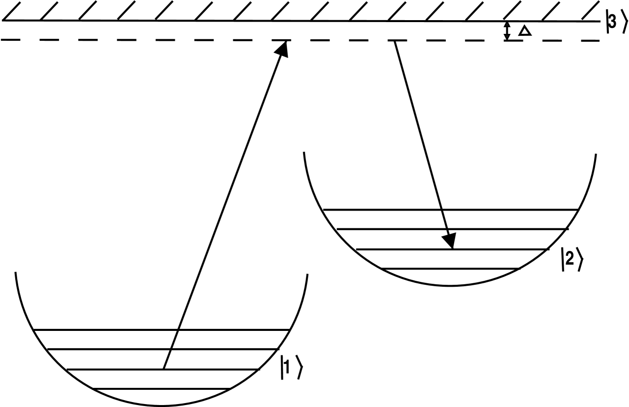
Figure 1: Raman process coupling two atomic hyperfine levels that may or may not be Bose-condensed.

A two-photon Bragg scattering experiment involves two laser beams at different frequencies and with different propagation vectors structure-factor-phonons-houches-exp . However, we are interested in a different type of two-photon process in which an atom changes its hyperfine state. This is a Raman process and is depicted in Fig. 1. We now discuss how the effective frequency $\omega$ and wavevector $\mathbf{q}$ in (3) are defined in such a Raman scattering experiment raman-output-coupler . Assuming that each laser beam has equal intensity $I$, the combined intensity of the two beams at space-time point $(\mathbf{r},t)$ is given by

$$I_{tot}(\mathbf{r},t)=2I+2I\cos(\mathbf{q}\cdot\mathbf{r}-\omega t),$$ (68)

where $\omega$ is the frequency difference between the two laser beams

$$\omega\equiv\omega_{a}-\omega_{b}.$$ (69)

The wavevector difference between the two laser beams is

$$\mathbf{q}=\mathbf{k}_{a}-\mathbf{k}_{b},$$ (70)

where $\mathbf{k}_{j}$ is the wavevector of laser beam $j$. We may take $k_{1}^{2}=k_{2}^{2}=\bar{k}^{2}$ such that the standard Bragg scattering relation (see, for example, p. 103 of Ref. ashcroft-mermin ) holds and $q$ is given by

$$q^{2}=4\bar{k}^{2}\sin^{2}\left(\frac{\theta}{2}\right),$$ (71)

where $\theta$ is the angle between the two counter-propagating beams. Finally the coupling parameter $\gamma$ in (3) is related to the single-photon Rabi frequency $\Omega_{Rabi}$ (assumed to be the same for both hyperfine level transitions) and the laser beam detuning $\Delta$ from the intermediate level $\left|3\right\rangle$ (see Fig. 1) according to raman-output-coupler

$$\gamma\propto\frac{\left|\Omega_{Rabi}\right|^{2}}{\Delta}\propto\Omega_{Rabi}^{(2)},$$ (72)

where $\Omega_{Rabi}^{(2)}$ is the so-called two-photon “Rabi frequency”.

The many-body Hamiltonian (in the absence of a tunneling perturbation) is $\hat{H}_{0}=\hat{H}_{10}+\hat{H}_{20}$, where

$$\hat{H}_{10}=\int\mathrm{d}\mathbf{r}\left\{\hat{\psi}_{1}^{\dagger}(\mathbf{r})\left[-\frac{\nabla^{2}}{2m}+U_{ext}(\mathbf{r})\right]\hat{\psi}_{1}(\mathbf{r})+\frac{g_{1}}{2}\hat{\psi}_{1}^{\dagger}(\mathbf{r})\hat{\psi}_{1}^{\dagger}(\mathbf{r})\hat{\psi}_{1}(\mathbf{r})\hat{\psi}_{1}(\mathbf{r})\right\}.$$ (73)

In this expression for $\hat{H}_{10}$, $U_{ext}$ is the trapping potential and $g_{1}=4\pi a_{1}/m$ is the s-wave scattering pseudo-potential with $a_{1}$ being the s-wave scattering length for atoms in gas $1$. The expression for $\hat{H}_{20}$ has an analogous form. We recall that the spectral densities in Section III are defined in terms of the grand canonical Hamiltonian $\hat{K}_{i0}\equiv\hat{H}_{i0}-\mu_{i}\hat{N}_{i}$. Thus the excitation energies of gas $i$ are measured relative to the chemical potential $\mu_{i}$.

IV.1 The Bogoliubov-Popov approximation

In the standard static Bogoliubov-Popov approximation for excitations in a trapped Bose gas fetter-walecka ; griffin-gapless ; rmp-bose-gas-review , the noncondensate field operator $\tilde{\psi}$ can be written as

$$\tilde{\psi}(\mathbf{r},t)=\sum_{j}\left(u_{j}(\mathbf{r})\mathrm{e}^{-iE_{j}t}\hat{\alpha}_{j}-v^{*}_{j}(\mathbf{r})\mathrm{e}^{iE_{j}t}\hat{\alpha}^{\dagger}_{j}\right),$$ (74)

where $u_{j}(\mathbf{r})$ and $v_{j}(\mathbf{r})$ are the Bogoliubov quasiparticle amplitudes, $E_{j}$ is the energy of Bogoliubov state $j$ and $\hat{\alpha}_{j}$ ($\hat{\alpha}^{\dagger}_{j}$) annihilate (create) a quasiparticle in state $j$, respectively. These annihilation and creation operators are defined to satisfy the boson commutation relations

$$\left[\hat{\alpha}_{m},\hat{\alpha}_{n}\right]=\left[\hat{\alpha}_{m}^{\dagger},\hat{\alpha}_{n}^{\dagger}\right]=0;\qquad\left[\hat{\alpha}_{m},\hat{\alpha}_{n}^{\dagger}\right]=\delta_{mn}.$$ (75)

The Bogoliubov quasiparticle amplitudes must satisfy the finite temperature coupled Bogoliubov-Popov equations of motion griffin-gapless

$$\hat{\mathcal{L}}u_{j}(\mathbf{r})-gn_{c}(\mathbf{r})v_{j}(\mathbf{r}) = E_{j}u_{j}(\mathbf{r})$$

$$\hat{\mathcal{L}}v_{j}(\mathbf{r})-gn_{c}(\mathbf{r})u_{j}(\mathbf{r}) = -E_{j}v_{j}(\mathbf{r})$$ (76)

in order for $\hat{K}_{0}$ to be reduced to the diagonal form

$$\hat{K}^{Bog}=const+\sum_{j}E_{j}\hat{\alpha}_{j}^{\dagger}\hat{\alpha}_{j}.$$ (77)

In (76), we have introduced the differential operator

$$\hat{\mathcal{L}}\equiv-\frac{\nabla^{2}}{2m}+U_{ext}(\mathbf{r})-\mu+2gn(\mathbf{r}),$$ (78)

where $n(\mathbf{r})$ is the total static density.

Using the commutation relations (75), one finds that the single-particle spectral density function can be expressed in terms of Bogoliubov quasiparticles as

$$A_{\tilde{\psi}^{\dagger}\tilde{\psi}}(\mathbf{r}^{\prime},\mathbf{r},t-t^{\prime})=\sum_{j}\Biggl{[}u^{*}_{j}(\mathbf{r}^{\prime})u_{j}(\mathbf{r})\mathrm{e}^{-iE_{j}(t-t^{\prime})}-v_{j}(\mathbf{r}^{\prime})v^{*}_{j}(\mathbf{r})\mathrm{e}^{iE_{j}(t-t^{\prime})}\Biggr{]},$$ (79)

which has the Fourier transform

$$A_{\tilde{\psi}^{\dagger}\tilde{\psi}}(\mathbf{r}^{\prime},\mathbf{r},\omega)=2\pi\sum_{j}\Biggl{[}u^{*}_{j}(\mathbf{r}^{\prime})u_{j}(\mathbf{r})\delta(\omega-E_{j})-v_{j}(\mathbf{r}^{\prime})v^{*}_{j}(\mathbf{r})\delta(\omega+E_{j})\Biggr{]}.$$ (80)

We note the appearance in (80) of negative energy poles ($\omega=-E_{j}$) in addition to the usual positive energy poles ($\omega=E_{j}$). These are a result of unique processes induced by the Bose condensate. The two poles follow immediately from (74), which shows how the destruction of an atom involves a linear superposition of the destruction (amplitude $u$) and creation (amplitude $v$) of Bogoliubov excitations.

Similarly, the off-diagonal or anomalous single-particle spectral density function of relevance to the anomalous current densities $i^{c-nc}_{A}$ in (66) and $i_{A}^{nc-nc}$ in (67) is given by

$$A_{\tilde{\psi}\tilde{\psi}}(\mathbf{r}^{\prime},\mathbf{r},\omega)=-2\pi\sum_{j}\Biggl{[}u_{j}(\mathbf{r})v_{j}^{*}(\mathbf{r}^{\prime})\delta(\omega-E_{j})-u_{j}(\mathbf{r}^{\prime})v_{j}^{*}(\mathbf{r})\delta(\omega+E_{j})\Biggr{]}.$$ (81)

The spectral density functions can be shown to satisfy $A_{\tilde{\psi}^{\dagger}\tilde{\psi}^{\dagger}}(\mathbf{r}^{\prime},\mathbf{r},\omega)=A^{*}_{\tilde{\psi}\tilde{\psi}}(\mathbf{r},\mathbf{r}^{\prime},\omega)$ and $A_{\tilde{\psi}^{\dagger}\tilde{\psi}}(\mathbf{r}^{\prime},\mathbf{r},\omega)=A^{*}_{\tilde{\psi}\tilde{\psi}^{\dagger}}(\mathbf{r},\mathbf{r}^{\prime},\omega)$.

IV.2 The normal and anomalous currents in the Bogoliubov-Popov approximation

Using the results in (80) and (81), we can now write the normal and anomalous linear response currents in terms of Bogoliubov excitations. In Section III, we found that two distinct physical processes contribute to the normal current. The current density of atoms tunneling between the condensates and noncondensates of the two gases is given by (54), or

$$i_{N}^{c-nc}(\mathbf{r},\mathbf{r}^{\prime},\omega) = 2\pi\sum_{j}\Bigg{[}\Phi^{*}_{10}(\mathbf{r})\Phi_{10}(\mathbf{r}^{\prime})u_{2j}^{*}(\mathbf{r})u_{2j}(\mathbf{r}^{\prime})\delta(\omega-E_{2j})$$ (82)

$$-\Phi_{10}^{*}(\mathbf{r}^{\prime})\Phi_{10}(\mathbf{r})v_{2j}(\mathbf{r}^{\prime})v^{*}_{2j}(\mathbf{r})\delta(\omega+E_{2j})$$

$$-\Phi^{*}_{20}(\mathbf{r}^{\prime})\Phi_{20}(\mathbf{r})u_{1j}^{*}(\mathbf{r}^{\prime})u_{1j}(\mathbf{r})\delta(\omega+E_{1j})$$

$$+\Phi_{20}^{*}(\mathbf{r})\Phi_{20}(\mathbf{r}^{\prime})v_{1j}(\mathbf{r})v^{*}_{1j}(\mathbf{r}^{\prime})\delta(\omega-E_{1j})\Bigg{]}.$$

This type of process involves both condensate atoms and quasiparticles. The current density associated with the tunneling of atoms between the noncondensates of the two gases has a more complicated form given by (55), or

$$i_{N}^{nc-nc}(\mathbf{r},\mathbf{r}^{\prime},\omega,\omega^{\prime}) = (2\pi)^{2}\biggl{(}N_{1}^{0}(\omega)-N_{2}^{0}(\omega^{\prime})\biggr{)}$$ (83)

$$\sum_{i,j}\Biggl{[}u^{*}_{1i}(\mathbf{r}^{\prime})u_{1i}(\mathbf{r})u_{2j}^{*}(\mathbf{r})u_{2j}(\mathbf{r}^{\prime})\delta(\omega-E_{1i})\delta(\omega^{\prime}-E_{2j})$$

$$-u_{1i}^{*}(\mathbf{r}^{\prime})u_{1i}(\mathbf{r})v_{2j}(\mathbf{r})v_{2j}^{*}(\mathbf{r}^{\prime})\delta(\omega-E_{1i})\delta(\omega^{\prime}+E_{2j})$$

$$-v_{1i}(\mathbf{r}^{\prime})v_{1i}^{*}(\mathbf{r})u_{2j}^{*}(\mathbf{r})u_{2j}(\mathbf{r}^{\prime})\delta(\omega+E_{1i})\delta(\omega^{\prime}-E_{2j})$$

$$+v_{1i}(\mathbf{r}^{\prime})v_{1i}^{*}(\mathbf{r})v_{2j}(\mathbf{r})v^{*}_{2j}(\mathbf{r}^{\prime})\delta(\omega+E_{1i})\delta(\omega^{\prime}+E_{2j})\Biggr{]}.$$

As in the case of the normal current, two different physical processes contribute to the anomalous current in (56). The first process involves pairs of condensate atoms tunneling to noncondensate states of the other Bose gas. This anomalous current density is given by (66), namely

$$i_{A}^{c-nc}(\mathbf{r},\mathbf{r}^{\prime},\omega) = 2\pi\sum_{j}\Biggl{[}\Phi_{10}(\mathbf{r}^{\prime})\Phi_{10}(\mathbf{r})u_{2j}(\mathbf{r})v^{*}_{2j}(\mathbf{r}^{\prime})\delta(\omega+E_{2j})$$ (84)

$$-\Phi^{*}_{10}(\mathbf{r}^{\prime})\Phi^{*}_{10}(\mathbf{r})u^{*}_{2j}(\mathbf{r}^{\prime})v_{2j}(\mathbf{r})\delta(\omega-E_{2j})$$

$$-\Phi^{*}_{20}(\mathbf{r})\Phi^{*}_{20}(\mathbf{r}^{\prime})u_{1j}(\mathbf{r}^{\prime})v^{*}_{1j}(\mathbf{r})\delta(\omega+E_{1j})$$

$$+\Phi^{*}_{20}(\mathbf{r})\Phi^{*}_{20}(\mathbf{r}^{\prime})u^{*}_{1j}(\mathbf{r})v_{1j}(\mathbf{r}^{\prime})\delta(\omega-E_{1j})\Biggr{]}.$$

The expression for the anomalous current density between condensate 1 and noncondensate 2 has a similar form. The final process involves quasiparticles of both gases and is given by (67), namely

$$i_{A}^{nc-nc}(\mathbf{r},\mathbf{r}^{\prime},\omega,\omega^{\prime}) = (2\pi)^{2}\biggl{(}N_{1}^{0}(\omega)-N_{2}^{0}(\omega^{\prime})\biggr{)}$$ (85)

$$\sum_{i,j}\Biggl{[}u_{1i}(\mathbf{r}^{\prime})v_{1i}^{*}(\mathbf{r})u_{2j}^{*}(\mathbf{r}^{\prime})v_{2j}(\mathbf{r})\delta(\omega+E_{1i})\delta(\omega^{\prime}+E_{2j})$$

$$-u_{1i}(\mathbf{r}^{\prime})v_{1i}^{*}(\mathbf{r})u_{2j}(\mathbf{r})v_{2j}^{*}(\mathbf{r}^{\prime})\delta(\omega+E_{1i})\delta(\omega^{\prime}-E_{2j})$$

$$-u^{*}_{1i}(\mathbf{r})v_{1i}(\mathbf{r}^{\prime})u_{2j}^{*}(\mathbf{r}^{\prime})v_{2j}(\mathbf{r})\delta(\omega-E_{1i})\delta(\omega^{\prime}+E_{2j})$$

$$+u^{*}_{1i}(\mathbf{r})v_{1i}(\mathbf{r}^{\prime})u_{2j}(\mathbf{r})v_{2j}^{*}(\mathbf{r}^{\prime})\delta(\omega-E_{1i})\delta(\omega^{\prime}-E_{2j})\Biggr{]}.$$

As with the Josephson current given in (31), one sees from (82)-(85) that the magnitude of the normal and anomalous quasiparticle currents is determined by the spatial overlap of the Bogoliubov wavefunctions described by $u_{i}(\mathbf{r})$ and $v_{i}(\mathbf{r})$ for the two systems.

When one uses (82)-(85) in the expressions for the normal (see (52) and (53)) and anomalous (see (59) and (60)) currents, our results are essentially equivalent to expressions discussed in Ref. finite-T-josephson . The main differences are that Meier and Zwerger approximated the two Bose gases as being uniform (or homogeneous) and used the single-particle spectral densities at $T=0$.

V Out-coupling to a non-Bose-condensed gas

In this section, we consider the special case of atoms out-coupling to the vacuum as discussed in Refs. burnett-1 ; burnett-2 . More precisely, we first deal with the case when gas 2 is a uniform non-interacting gas. The corresponding spectral density function then has the well-known form kadanoff-and-baym ; fetter-walecka

$$A_{\hat{\psi}_{2}^{\dagger}\hat{\psi}_{2}}(\mathbf{k},\omega)=2\pi\delta\left(\omega-\tilde{\varepsilon}_{\mathbf{k}2}\right),$$ (86)

where

$$\tilde{\varepsilon}_{\mathbf{k}2}\equiv k^{2}/2m-\mu_{2}$$ (87)

is the the excitation energy of an atom in gas $2$. Because the gas is assumed to be in the classical limit, we have $N_{2}^{0}(\tilde{\varepsilon}_{\mathbf{k}2})\ll 1$.

The only terms in (82) which are finite reduce to

$$i_{Nout}^{c-nc}(\mathbf{r},\mathbf{r}^{\prime},\omega) = \Phi_{10}^{*}(\mathbf{r}^{\prime})\Phi_{10}(\mathbf{r})A_{\tilde{\psi}_{2}^{\dagger}\tilde{\psi}_{2}}(\mathbf{r}-\mathbf{r}^{\prime},\omega)$$ (88)

$$= 2\pi\int\frac{\mathrm{d}\mathbf{k}}{(2\pi)^{3}}\mathrm{e}^{-i\mathbf{k}\cdot(\mathbf{r}-\mathbf{r}^{\prime})}\Phi_{10}^{*}(\mathbf{r}^{\prime})\Phi_{10}(\mathbf{r})\delta(\tilde{\varepsilon}_{\mathbf{k}2}-\omega)$$

and in (83)

$$i_{Nout}^{nc-nc}(\mathbf{r},\mathbf{r}^{\prime},\omega,\omega^{\prime}) = N_{1}^{0}(\omega)A_{\tilde{\psi}_{1}^{\dagger}\tilde{\psi}_{1}}(\mathbf{r}^{\prime},\mathbf{r},\omega)A_{\tilde{\psi}_{2}^{\dagger}\tilde{\psi}_{2}}(\mathbf{r}-\mathbf{r}^{\prime},\omega^{\prime})$$ (89)

$$= 4\pi^{2}\sum_{j}\int\frac{\mathrm{d}\mathbf{k}}{(2\pi)^{3}}\biggl{\{}N_{1}^{0}(E_{1j})u^{*}_{1j}(\mathbf{r}^{\prime})u_{1j}(\mathbf{r})\delta\left(\omega-E_{1j}\right)$$

$$+[1+N_{1}^{0}(E_{1j})]v_{1j}(\mathbf{r}^{\prime})v^{*}_{1j}(\mathbf{r})\delta\left(\omega+E_{1j}\right)\biggr{\}}\delta(\tilde{\varepsilon}_{\mathbf{k}2}-\omega^{\prime}).$$

We have used the Bose identity $N^{0}(-\omega)=-[1+N^{0}(\omega)]$ in writing the last term in (89). The condition that $N_{2}^{0}\ll 1$ results in negligible tunneling from gas 2 back to gas 1.

The current density $i_{Nout}^{(c-nc)}$ in (88) corresponds to the destruction of a condensate atom in gas $1$ and the creation of an excitation in gas $2$ with energy $\tilde{\varepsilon}_{\mathbf{k}2}$. The first term in the density $i_{Nout}^{(nc-nc)}$ of (89) represents what might be called the “quantum evaporation” of an atom, destroying a Bogoliubov quasiparticle with energy $E_{1j}=k^{2}/2m-(\omega-\Delta\varepsilon+\mu_{1})$ and creating an atom in gas $2$ with $k^{2}/2m$. The second term in (89) corresponds to creating an atom in gas $2$ with energy $k^{2}/2m$ and simultaneously creating a quasiparticle excitation in gas $1$ with energy $E_{1j}=-[k^{2}/2m-(\omega-\Delta\varepsilon+\mu_{1})]$. This second out-coupling channel in (89) is a direct consequence of the unusual condensate-induced correlations in a Bose gas. It corresponds to the “pair-breaking” process discussed by the Oxford group burnett-1 . The analogue of this process appears in the predicted lineshape of the recombination photons emitted in the decay of an exciton in a Bose-condensed gas of optically-excited excitons svg . All three out-coupling contributions will be calculated in Section VI.

Using (88) and (89), the out-coupling current $\delta I_{out}$ is

$$\delta I_{out} = \gamma^{2}\int\mathrm{d}\mathbf{r}\int\mathrm{d}\mathbf{r}^{\prime}\int\frac{\mathrm{d}\mathbf{k}}{(2\pi)^{3}}\mathrm{e}^{i(\mathbf{q}-\mathbf{k})\cdot(\mathbf{r}-\mathbf{r}^{\prime})}$$ (90)

$$\qquad\Biggl{\{}\Phi_{10}^{*}(\mathbf{r}^{\prime})\Phi_{10}(\mathbf{r})\delta\left(k^{2}/2m-(\omega-\Delta\varepsilon+\mu_{1})\right)$$

$$+2\pi\sum_{j}\biggl{[}N_{1}^{0}(E_{1j})u_{1j}^{*}(\mathbf{r}^{\prime})u_{1j}(\mathbf{r})\delta\left(k^{2}/2m-(\omega-\Delta\varepsilon+\mu_{1})-E_{1j}\right)$$

$$\qquad+[1+N_{1}^{0}(E_{1j})]v_{1j}(\mathbf{r}^{\prime})v^{*}_{1j}(\mathbf{r})\delta\left(k^{2}/2m-(\omega-\Delta\varepsilon+\mu_{1})+E_{1j}\right)\biggr{]}\Biggr{\}}.$$

We refer to the second term as the “$u^{2}$ contribution” and the third term as the “$v^{2}$ contribution”. It is useful to describe the main features of the out-coupling current spectrum arising from the three terms in (90), as a function of the energy $k^{2}/2m$ of the out-coupled atoms, for fixed $\omega$ and $\mathbf{q}$. The energy conserving delta functions in (90) determine the energies of the out-coupling current peaks for the different processes. There is a delta function peak at $k^{2}/2m+\varepsilon_{2}=\omega+\varepsilon_{1}+\mu_{1}$ from atoms coming directly from the condensate, where $\mu_{1}$ is the condensate energy of a trapped atom in the hyperfine state $\left|1\right\rangle$ and $\varepsilon_{i}$ is the hyperfine state energy. Relative to this condensate pole, the peak associated with the quantum evaporation term is shifted by a positive amount $E_{1j}$, while the peak of the “pair-breaking” channel is shifted by a negative amount $-E_{1j}$. These shifts follow from the fact that the quantum evaporation channel arises from the positive energy pole (related to $u^{2}$) and the pair-breaking channel corresponds to the negative energy pole (related to $v^{2}$) in the single-particle spectral density.

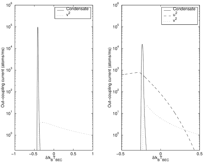
Figure 2: Out-coupling atom current for $a\simeq 5\,nm$ and $q=2/a_{HO}$. The detuned frequency $\delta$ is defined in (94). The plot on the left is at $T=0$. The plot on the right is at $T=0.9T_{BEC}$. In Figs. 2-5, we take $N=10^{6}$ atoms, $\omega_{0}=2\pi\times 60\,Hz$ and $\gamma=0.2\omega_{0}$.

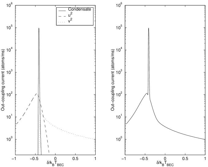
Figure 3: Out-coupling atom current for $a\simeq 5\,nm$ and $q=2/a_{HO}$. The plot on the left shows each component contributing to the out-coupling atom current. The plot on the right shows the total out-coupling atom current. In both plots $T=0.2T_{BEC}$.

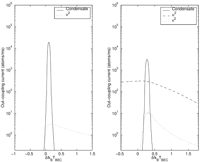
Figure 4: Out-coupling current for $a\simeq 5\,nm$ and $q=10/a_{HO}$. The plot on the left is at $T=0$. The plot on the right is at $T=0.9T_{BEC}$.

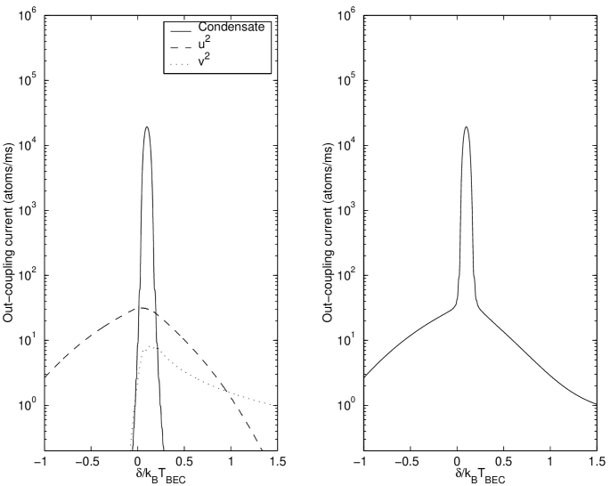
Figure 5: Out-coupling atom current for $a\simeq 5\,nm$ and $q=10/a_{HO}$. The plot on the left shows each component contributing to the out-coupling atom current. The plot on the right shows the total out-coupling atom current. In both plots $T=0.2T_{BEC}$.

We next consider the behavior of the three out-coupling current contributions in (90) as a function of temperature. For $T_{1}=0$, since $N_{1}^{0}(E_{1j})\rightarrow 0$, (i.e. no thermally excited quasiparticles) the second channel ($u^{2}$) has zero weight. Thus, at $T_{1}=0$, only the first and third processes occur. When gas 1 is at a finite temperature ($T_{1}\neq 0$), the second channel ($u^{2}$) begins to contribute to the out-coupling current, taking weight away from the pair-breaking channel ($v^{2}$). All these features are shown explicitly in the numerical results given in Section VI (see Figs. 2-5).

The out-coupling current derived in Ref. burnett-2 is given as the rate of atoms excited out of gas 1 with energy $\tilde{\varepsilon}_{\mathbf{k}2}$ and may be written as (where we use a notation more consistent with our own)

$$\frac{\mathrm{d}n_{\mathbf{k}}}{\mathrm{d}t} = \gamma^{2}\int\mathrm{d}\mathbf{r}\int\mathrm{d}\mathbf{r}^{\prime}\mathrm{e}^{i\mathbf{q}\cdot(\mathbf{r}-\mathbf{r}^{\prime})}\varphi^{*}_{\mathbf{k}2}(\mathbf{r})\varphi_{\mathbf{k}2}(\mathbf{r}^{\prime})$$ (91)

$$\qquad\times\Biggl{\{}\Phi^{*}_{10}(\mathbf{r}^{\prime})\Phi_{10}(\mathbf{r})\delta\left(k^{2}/2m-(\omega-\Delta\varepsilon+\mu_{1})\right)$$

$$+2\pi\sum_{j}\biggl{[}N^{0}_{1}(E_{1j})u^{*}_{1j}(\mathbf{r}^{\prime})u_{1j}(\mathbf{r})\delta\left(k^{2}/2m-(\omega-\Delta\varepsilon+\mu_{1})-E_{1j}\right)$$

$$\qquad+[1+N^{0}_{1}(E_{1j})]v_{1j}(\mathbf{r}^{\prime})v^{*}_{1j}(\mathbf{r})\delta\left(k^{2}/2m-(\omega-\Delta\varepsilon+\mu_{1})+E_{1j}\right)\biggr{]}\Biggr{\}},$$

where $\varphi_{\mathbf{k}2}(\mathbf{r})$ is the wavefunction for the out-coupled excitation with energy $\tilde{\varepsilon}_{\mathbf{k}2}$. We can make a direct comparison between the integrands of (90) and (91). Indeed taking $\varphi_{2\mathbf{k}}(\mathbf{r})=e^{i\mathbf{k}\cdot\mathbf{r}}$ (a free atom with momentum $\mathbf{k}$) reduces (91) to the integrand of (90). Thus our result for the out-coupling current reduces to that derived in Refs. burnett-1 ; burnett-2 , where the out-coupled atoms were in free-particle states.

VI The Local Density Approximation (LDA)

In this section, we evaluate the out-coupling current in (90) and estimate the magnitude and temperature-dependence of the quantum evaporation and pair-breaking effects discussed in Section V. In previous work burnett-1 ; burnett-2 , these noncondensate processes were found to be a few percent, relative to the dominant contribution of atoms tunneling out of the high density condensate. It has also been found unpublished-structure-factor-finite-T that in current Bose gas experiments, the contribution of the noncondensate atoms to the dynamic structure factor $S(\mathbf{q},\omega)$ at $T=0.9T_{BEC}$ is about $5\,\%$ of the contribution from the condensate fluctuations (the latter has been studied in Refs. structure-factor-phonons-exp ; structure-factor-phonons-houches-exp ; trento-dynamic-structure-factor at $T=0$). This small amplitude is, of course, a direct reflection of the strongly peaked condensate at the centre of the trap compared to the broad, low density profile of the noncondensate atoms. However, while small, the tunneling current from the noncondensate atoms gives direct information about the Bose-induced correlations and thus is a worthwhile goal for future Bragg scattering and Raman experiments.

The condensate current in (90) can be rewritten in the form

$$\delta I_{out}^{c}(\mathbf{q},\delta)\equiv\gamma^{2}\int\frac{\mathrm{d}\mathbf{k}}{(2\pi)^{3}}\left|\Phi_{10}(\mathbf{q}-\mathbf{k})\right|^{2}\delta(\nu_{\mathbf{k}}),$$ (92)

where $\Phi_{10}(\mathbf{q}-\mathbf{k})$ is the Fourier transform of the Bose order parameter

$$\Phi_{10}(\mathbf{q}-\mathbf{k})\equiv\int\mathrm{d}\mathbf{r}\mathrm{e}^{i(\mathbf{q}-\mathbf{k})\cdot\mathbf{r}}\Phi_{10}(\mathbf{r})$$ (93)

and we have introduced the abbreviation $\nu_{\mathbf{k}}\equiv k^{2}/2m-(\omega-\Delta\varepsilon)-\mu_{1TF}$. It is also useful to introduce a “detuned frequency”

$$\delta\equiv\omega-\Delta\varepsilon.$$ (94)

The noncondensate contribution in (90) is more conveniently written in terms of the trapped gas Bogoliubov spectral density in (80),

$$\delta I_{out}^{nc}(\mathbf{q},\delta)=\gamma^{2}\int\mathrm{d}\mathbf{r}\int\mathrm{d}\mathbf{r}^{\prime}\int\frac{\mathrm{d}\mathbf{k}}{(2\pi)^{3}}\mathrm{e}^{i(\mathbf{q}-\mathbf{k})\cdot(\mathbf{r}-\mathbf{r}^{\prime})}N_{1}^{0}(\nu_{\mathbf{k}})A_{\tilde{\psi}_{1}^{\dagger}\tilde{\psi}_{1}}(\mathbf{r}^{\prime},\mathbf{r},\nu_{\mathbf{k}}).$$ (95)

In the rest of this section, for notational simplicity, we shall drop the index “1” on the quantities associated with the trapped gas. Equations (92) and (95) summarize our main results for the tunneling currents into the vacuum, showing very clearly which properties of the trapped Bose gas they depend on.

VI.1 Condensate contribution

In the standard Thomas-Fermi approximation, the condensate density profile is given by rmp-bose-gas-review

$$n_{c0}(\mathbf{r})=\left\{\begin{array}[]{ccc}\biggr{(}\mu_{TF}-U_{ext}(\mathbf{r})\biggl{)}/g,&r\leq R_{TF}&\\ 0,&r>R_{TF}\end{array}\right.,$$ (96)

where the chemical potential is

$$\mu_{TF}=\frac{1}{2}m\omega_{0}^{2}R_{TF}^{2},$$ (97)

and

$$R_{TF}=a_{HO}\left(15N_{c}(T)\frac{a}{a_{HO}}\right)^{1/5}.$$ (98)

The Thomas-Fermi radius $R_{TF}$ defines the size of the condensate, with $N_{c}(T)$ the total number of particles in the Bose-condensate at temperature $T$ and $a_{HO}=\sqrt{\hbar/m\omega_{0}}$ is the oscillator length. The $T=0$ Thomas-Fermi results have been extended to finite temperature by adjusting $N_{c}$ according to the noninteracting trapped gas result rmp-bose-gas-review

$$\frac{N_{c}(T)}{N}=1-\left(\frac{T}{T_{BEC}}\right)^{3},$$ (99)

where $k_{B}T_{BEC}\equiv 0.94\hbar\omega_{0}N^{1/3}$ is the noninteracting trapped gas Bose-condensation temperature. Using (96) for the order parameter $\Phi_{0}(\mathbf{r})=\sqrt{n_{c0}(\mathbf{r})}$, the Fourier transform in (93) can be calculated analytically

$$\Phi_{0}(\mathbf{k}) = 4\pi\int_{0}^{\infty}\mathrm{d}r\,r\sqrt{n_{c0}(r)}\frac{\sin(kr)}{k}$$ (100)

$$= \frac{2\pi^{2}R_{TF}^{2}}{\sqrt{2g}k^{2}}J_{2}(kR_{TF}),$$

where $J_{2}$ is the ordinary Bessel function of order 2. This result is the same as previously obtained baym-momentum-condensate-tf ; trento-dynamic-structure-factor , taking into account that we use harmonic oscillator units (length is measured in units of $a_{HO}=\sqrt{\hbar/m\omega_{0}}$ and energy is measured in terms of $\hbar\omega_{0}$).

Writing the integral in (92) in terms of spherical coordinates, we obtain using (100)

$$\delta I_{out}^{c}(\mathbf{q},\delta) = \frac{\gamma^{2}}{2\pi\omega_{0}}\frac{\big{(}gn_{c0}(\mathbf{r}=0)\big{)}^{7/2}}{g}$$ (101)

$$\times\frac{1}{q}\int^{x_{+}}_{x_{-}}\mathrm{d}x\frac{J_{2}^{2}(x)}{x^{4}}\theta(\delta+\mu_{TF}),$$

where $x_{\pm}=\sqrt{2gn_{c0}(\mathbf{r}=0)}\bigg{(}q\pm\sqrt{2(\delta+\mu_{TF})}\bigg{)}^{2}$. The result (101) may be easily generalized to asymmetric harmonic traps, having trapping potential

$$U_{ext}(\mathbf{r})=\frac{1}{2}m\bigg{(}\omega_{x}^{2}x^{2}+\omega^{2}_{y}y^{2}+\omega_{z}^{2}z^{2}\bigg{)},$$ (102)

by introducing the coordinate transformation

$$x=\frac{\bar{\omega}}{\omega_{x}}x^{\prime},\quad y=\frac{\bar{\omega}}{\omega_{y}}y^{\prime},\quad z=\frac{\bar{\omega}}{\omega_{z}}z^{\prime},$$ (103)

where $\bar{\omega}\equiv(\omega_{x}\omega_{y}\omega_{z})^{1/3}$. The same procedure as used above follows through with the same final expressions, apart from $\omega_{0}$ being replaced by $\bar{\omega}$. In addition, any wavevector $\mathbf{k}$ in our tunneling expressions such as (92) needs to be interpreted as $\mathbf{k}\rightarrow\left(\frac{\bar{\omega}}{\omega_{x}}k_{x},\frac{\bar{\omega}}{\omega_{y}}k_{y},\frac{\bar{\omega}}{\omega_{z}}k_{z}\right)$ in an anisotropic trap trento-dynamic-structure-factor .

The total out-coupling current from the condensate given by (92), as a function of the detuning parameter $\delta$ in (94), is shown by the solid lines in Figs. 2 and 3. In all our numerical calculations, for the two-photon Rabi coupling we have used $\gamma=0.2\omega_{0}$. Note the logarithmic scale for the out-coupled atom current. The current magnitude only decreases as a function of increasing temperature by about $20\,\%$. From Fig. 4, it can be seen that the maximum condensate tunneling current amplitude is sensitive to the magnitude of the momentum transfer $\mathbf{q}$. The decrease in the maximum tunneling current with increasing values of $q$ is a result of the fact that the momentum distribution of atoms in the condensate is peaked at zero momentum, decreasing for increasing momentum. For an asymmetric trap, this means that the directions of strongest confinement (largest trap frequency) will out-couple most efficiently. We observe also that the peak of the condensate tunneling current shifts toward positive $\delta$ as $q$ increases.

VI.2 Noncondensate contribution

The out-coupling current (95) from the noncondensate atoms will be estimated using a simple local density approximation (LDA). The LDA has also been recently used to calculate $S(\mathbf{q},\omega)$ in trapped gases timmermans-tommasini-structure-factor-lda ; trento-dynamic-structure-factor . We first introduce a new coordinate system defined in terms of the relative coordinate

$$\bar{\mathbf{r}}=\mathbf{r}-\mathbf{r}^{\prime}$$ (104)

and the center-of-mass coordinate

$$\mathbf{R}=\frac{\mathbf{r}+\mathbf{r}^{\prime}}{2}.$$ (105)

Writing the single-particle spectral density function $A_{\tilde{\psi}^{\dagger}\tilde{\psi}}(\mathbf{r},\mathbf{r}^{\prime},\omega)$ in (95) in terms of these new coordinates, we note that for large condensates and quasiparticle energies much larger than $\hbar\omega_{0}$, the spectral density will vary slowly as a function of $\mathbf{R}$. It is thus plausible to approximate $A_{\tilde{\psi}^{\dagger}\tilde{\psi}}$ by its homogeneous form, but adjusted so that at each point $\mathbf{R}$ the appropriate condensate density $n_{c0}(\mathbf{R})$ is used. Thus, in the LDA, the single-particle spectral density function in (95) is approximated by

$$A_{\tilde{\psi}^{\dagger}\tilde{\psi}}(\mathbf{r},\mathbf{r}^{\prime},\omega)=A_{\tilde{\psi}^{\dagger}\tilde{\psi}}(\bar{\mathbf{r}},\mathbf{R},\omega)\simeq A_{\tilde{\psi}^{\dagger}\tilde{\psi}}^{LDA}(\bar{\mathbf{r}},\omega;n_{c0}(\mathbf{R})),$$ (106)

where $A_{\tilde{\psi}^{\dagger}\tilde{\psi}}^{LDA}$ denotes the uniform gas expression for the spectral density function for a condensate density $n_{c0}$.

In the Bogoliubov-Popov approximation, the LDA form (106) for the spectral density in energy-momentum space is giorgini-popov-and-semiclassical

$$A_{\tilde{\psi}^{\dagger}\tilde{\psi}}^{LDA}(\mathbf{p},\omega;n_{c0}(\mathbf{R})) = 2\pi\Biggl{[}u^{2}(\mathbf{p};n_{c0}(\mathbf{R}))\delta\biggl{(}\omega-E(\mathbf{p};n_{c0}(\mathbf{R}))\biggr{)}$$ (107)

$$-v^{2}(\mathbf{p};n_{c0}(\mathbf{R}))\delta\biggl{(}\omega+E(\mathbf{p};n_{c0}(\mathbf{R}))\biggr{)}\Biggr{]}.$$

Thus, in the LDA the quasiparticle energies become

$$E(\mathbf{p};n_{c0}(\mathbf{R}))=\left\{\begin{array}[]{ccc}\sqrt{\varepsilon_{\mathbf{p}}^{2}+2\mu_{eff}(\mathbf{R})\varepsilon_{\mathbf{p}}},&R\leq R_{TF}&\\ \varepsilon_{\mathbf{p}}-\mu_{eff}(\mathbf{R}),&R>R_{TF}\end{array}\right.,$$ (108)

while the Bogoliubov quasiparticle mode amplitudes are given by

$$u^{2}(\mathbf{p};n_{c0}(\mathbf{R})) = \left\{\begin{array}[]{ccc}\frac{\varepsilon_{\mathbf{p}}-\mu_{eff}(\mathbf{R})}{2E(\mathbf{p};n_{c0}(\mathbf{R}))}+\frac{1}{2},&R\leq R_{TF}&\\ 1,&R>R_{TF}\end{array}\right.$$ (111)

$$v^{2}(\mathbf{p};n_{c0}(\mathbf{R})) = \left\{\begin{array}[]{ccc}\frac{\varepsilon_{\mathbf{p}}-\mu_{eff}(\mathbf{R})}{2E(\mathbf{p};n_{c0}(\mathbf{R}))}-\frac{1}{2},&R\leq R_{TF}&\\ 0,&R>R_{TF}\end{array}\right..$$ (114)

We have introduced the free atom energy $\varepsilon_{\mathbf{p}}\equiv p^{2}/2m$ and

$$\mu_{eff}(\mathbf{R})\equiv\mu_{TF}-U_{ext}(\mathbf{R})-2gn_{c0}(\mathbf{R}),$$ (115)

plays the role of an “effective” local chemical potential, modifying the chemical potential $\mu_{TF}$ as a result of the inhomogeneity of the trap.

Within the LDA, the noncondensate contribution (95) to the out-coupling current is given by

$$\delta I_{out}^{nc}(\mathbf{q},\delta)=\frac{\gamma^{2}}{\omega_{0}}\int\frac{\mathrm{d}\mathbf{k}}{(2\pi)^{3}}N^{0}(\nu_{\mathbf{k}})\int\mathrm{d}\mathbf{R}A^{LDA}_{\tilde{\psi}^{\dagger}\tilde{\psi}}(\mathbf{q}-\mathbf{k},\nu_{\mathbf{k}};n_{c0}(\mathbf{R})),$$ (116)

where as before we have introduced the variable $\nu_{\mathbf{k}}\equiv\varepsilon_{\mathbf{k}}-\delta-\mu_{TF}$ for notational simplicity. Using the identity

$$\delta(f(x))=\sum_{i}\frac{1}{\left|f^{\prime}(x_{i})\right|}\delta(x-x_{i}),$$ (117)

where $f(x_{i})=0$, we may evaluate the integral over $\mathbf{R}$ in (116) assuming a spherically symmetric trap. After some algebra, one obtains the following expression for the noncondensate contribution to the out-coupling current

$$\delta I_{out}^{nc}(\mathbf{q},\delta)=\frac{2\pi\gamma^{2}}{\omega_{0}}\int\frac{\mathrm{d}\mathbf{k}}{(2\pi)^{3}}N^{0}(\nu_{\mathbf{k}})\bar{A}^{LDA}_{\tilde{\psi}^{\dagger}\tilde{\psi}}(\mathbf{q}-\mathbf{k},\nu_{\mathbf{k}}),$$ (118)

where we have introduced the LDA spatially averaged spectral density function in energy-momentum space

$$\bar{A}^{LDA}_{\tilde{\psi}^{\dagger}\tilde{\psi}}(\mathbf{k},\omega) \equiv \int\mathrm{d}\mathbf{R}A^{LDA}_{\tilde{\psi}^{\dagger}\tilde{\psi}}(\mathbf{k},\omega;n_{c0}(\mathbf{R}))$$ (119)

$$= 2\pi\sqrt{2\bigg{(}\mu_{TF}-\mu(\mathbf{k},\omega)\bigg{)}}\left(\frac{\varepsilon_{\mathbf{k}}^{2}+\omega^{2}}{2\varepsilon_{\mathbf{k}}^{2}}+\frac{\left|\omega\right|}{\varepsilon_{\mathbf{k}}}\right)\theta(\omega)\theta\Biggl{(}\mu(\mathbf{k},\omega)\biggl{(}\mu_{TF}-\mu(\mathbf{k},\omega)\biggr{)}\Biggr{)}$$

$$+2\pi\sqrt{2\bigg{(}\mu_{TF}-\mu(\mathbf{k},\omega)\bigg{)}}\left(-\frac{\varepsilon_{\mathbf{k}}^{2}+\omega^{2}}{2\varepsilon_{\mathbf{k}}^{2}}+\frac{\left|\omega\right|}{\varepsilon_{\mathbf{k}}}\right)\theta(-\omega)\theta\Biggl{(}\mu(\mathbf{k},\omega)\biggl{(}\mu_{TF}-\mu(\mathbf{k},\omega)\biggr{)}\Biggr{)}$$

$$+4\pi\sqrt{2(\omega-\varepsilon_{\mathbf{k}}+\mu_{TF})}\theta(\omega-\varepsilon_{\mathbf{k}}),$$

where

$$\mu(\mathbf{k},\omega)\equiv\frac{\omega^{2}-\varepsilon_{\mathbf{k}}^{2}}{2\varepsilon_{\mathbf{k}}}$$ (120)

and harmonic oscillator units are used. Note that the noncondensate out-coupling current in (118) may be generalized to an asymmetric trap in the same manner as discussed earlier for the condensate out-coupling current (see remarks below (103)).

The formula in (118) has a simple physical interpretation. The integrand gives the number of emitted atoms with momentum $\mathbf{k}$ per second. The first term in (119) is associated with the positive energy pole in (80), with amplitude $u^{2}$, and only occurs for positive frequency $\omega>0$. The second term in (119) arises from the negative energy pole in (80), with amplitude $v^{2}$, and only occurs for negative frequency $\omega<0$. These first two terms are associated with quasiparticles in the region of the (Thomas-Fermi) condensate, i.e. for $R\leq R_{TF}$. The third term, in contrast, is associated with quasiparticles lying outside of the condensate region. These quasiparticles comprise a Hartree-Fock gas in our simple model calculation. The dominant weight in (119) comes from small $\varepsilon_{\mathbf{k}}$ and $\omega$. The quasiparticles with $u^{2}$ and $v^{2}$ weights in the region where there is a condensate are the dominant contribution. For $\omega>\varepsilon_{\mathbf{k}}(>0)$, one also finds a contribution from the normal Hartree-Fock gas of atoms existing outside of the condensate. As the temperature increases toward $T_{BEC}$, this contribution from the normal Hartree-Fock gas becomes more significant relative to the Bogoliubov quasiparticles. Of course, for $T>T_{BEC}$, it is the sole contribution.

We have evaluated the integral appearing in (118) numerically. Some results, as a function of the detuning parameter $\delta$ for various temperatures, are shown in Figs. 2 and 3. Note the logarithmic scale for the out-coupled atom current. As a function of detuning, the out-coupling current separates into two regions. From (118) and (119), we observe that for $\delta<-\mu_{TF}$ (or $\omega+\varepsilon_{1}+\mu_{TF}<\varepsilon_{2}$), we have $\nu_{\mathbf{k}}>0$ for all values of the wavevector $\mathbf{k}$. In this region, we find a contribution from the $u^{2}$ Bogoliubov modes, in addition to a smaller contribution from the atoms coming from outside the condensate region, at finite temperatures. This contribution to the out-coupling current $\delta I_{N}^{nc}$ represents the “quantum evaporation” process discussed at the end of Section V, being associated with positive energy poles of the single-particle noncondensate Green’s function. It is only present at finite temperatures. In Fig. 3, we have plotted the total out-coupling current as a function of the detuning $\delta$ at an intermediate temperature of $T=0.2T_{BEC}$.

However, for $\delta>-\mu_{TF}$ (or $\omega+\varepsilon_{1}+\mu_{TF}>\varepsilon_{2}$), $\nu_{\mathbf{k}}$ can be less than zero for a restricted set of wavevectors $\mathbf{k}$. In this case, there are two contributions to the out-coupling current $\delta I_{N}^{nc}$. One arises from the $v^{2}$ Bogoliubov modes and hence represents the so-called pair-breaking process associated with the negative energy poles of the single-particle noncondensate spectral density function (i.e., a tunneling atom creates a Bogoliubov excitation in the trapped gas). This is the only process which contributes to the noncondensate out-coupling current at zero temperature. At finite temperature, a second process arises which is associated with quantum evaporation from high momentum states. This involves the positive energy poles of the single-particle noncondensate spectral density function. This second contribution decays more quickly as the detuning is increased, compared with the $v^{2}$ contribution. We note that these two regions will be Doppler shifted toward positive $\delta$ by the nonzero momentum kick $\mathbf{q}$ from the laser fields. The overall behavior of our LDA results in Figs. 2-5 is similar to that reported in Refs. burnett-1 ; burnett-2 , which were based on solving a one-dimensional Gross-Pitaevskii equation for an isotropic trap.

We have also evaluated the noncondensate contribution to the out-coupling current for $q=10/a_{HO}$, with the results shown in Figs. 4 and 5. We observe that the point at which there is no longer any contribution from the $v^{2}$ Bogoliubov modes shifts increasingly toward positive $\delta$ as $q$ is increased. However, unlike for the case of $q=2/a_{HO}$, the contribution at finite temperatures from the $u^{2}$ Bogoliubov modes dominates that from the $v^{2}$ Bogoliubov modes for the range of $\delta$ considered. This results from the fact that the higher momentum quasiparticles have greater spectral weight. We have plotted the total out-coupling current at a temperature of $T=0.2T_{BEC}$ in Fig. 5.

Because of the strength of the condensate contribution, some comment is required about the observability of the noncondensate contribution in the total out-coupling current. Since the contribution from the condensate is smallest at high $q$, we compare the condensate and noncondensate contributions at a momentum kick of $q=10/a_{HO}$ (see Fig. 4). Since the out-coupling current as a function of $\delta$ is much broader for the noncondensate contribution than the condensate contribution, there are regions in which the strong contribution from the condensate will not dwarf that from the noncondensate. At $T=0.9T_{BEC}$, the maximum contribution from the quantum evaporation process is about $10\,\%$ of the maximum contribution from the condensate (see Fig. 4). The small but interesting $v^{2}$ Bogoliubov contribution is perhaps more visible as a “distinct contribution” in the limit of very low temperatures (see the $T=0$ results in Figs. 2 and 4).

The unique features associated with the out-coupled atoms coming from the noncondensate can also be enhanced by working with larger values of the s-wave scattering length $a$. In particular, one can “tune” the scattering length $a$ significantly by the use of Feshbach resonances stoof-feshbach-resonance-2 ; ketterle-feshbach-1 . The amplification of the out-coupling current of atoms associated with the negative energy poles of the single-particle noncondensate Green’s function could be looked for in trapped gases near a Feshbach resonance. Out-coupling experiments may thus provide important information about the Bose-condensed gas excitation spectrum if we can increase the s-wave scattering length substantially. In this case, of course, we expect observable changes from the simple Bogoliubov-Popov approximation we introduced in Section IV for the single-particle spectral density. Such many-body effects can thus be probed “directly” using the out-coupling kind of experiment we have been discussing.

VII Conclusions

This paper has studied the weak coupling of two trapped dilute Bose gases using a tunneling Hamiltonian approach. When considering tunneling between two trapped condensates, we obtained a coherent Josephson-type time-dependent contribution given in (31), with a frequency $\Omega\equiv\omega-\Delta\varepsilon-\Delta\mu$ (see also Ref. finite-T-josephson ). The expression in (31), which corresponds to coherent transfer of atoms between two condensates, is first order in the coupling $\gamma$. In addition, we found that two types of quasiparticle currents emerge from treating a perturbation of the kind shown in (3) to second order: a static, time-independent current given by (40) and (41) involving only regular correlation functions of the form $\left\langle\widetilde{\psi}^{\dagger}\widetilde{\psi}\right\rangle$, and a time-dependent current given by (59) and (60) involving a second harmonic with frequency $2\Omega$. The latter is associated with anomalous correlation functions of the kind $\left\langle\widetilde{\psi}\widetilde{\psi}\right\rangle$, and is reminiscent of the Josephson current carried by Cooper pairs in superconductors mahan . These tunneling currents were written in terms of single-particle spectral density functions that contain all the details of the microscopic correlations of the Bose-condensed gases. In this manner, the tunneling dynamics is cleanly separated from the specific approximation used for the many-body description of the Bose-condensed gas. This separation was one of the main goals of our work.

Our paper further serves to unify and extend the work of Ref. finite-T-josephson on Josephson-type and other kinds of tunneling phenomena in trapped Bose gases, as well as recent work burnett-1 ; burnett-2 dealing with out-coupling from a single Bose-condensed gas. It provides a transparent way of expressing the various contributions to the tunneling processes involving an inhomogeneous trapped Bose gas, before any specific approximation is introduced. The present paper thus provides a foundation upon which one can study the details of different tunneling processes within various many-body approximations for the dynamics of a Bose gas. Our work re-emphasizes the potential usefulness of the kind of out-coupling experiments discussed in Refs. burnett-1 ; burnett-2 as a probe of the many-body physics of a Bose-condensed gas, including systems of reduced dimensionality.

As we have noted in the text, our present study contrasts with the work reported in Refs. structure-factor-phonons-exp ; structure-factor-phonons-houches-exp ; timmermans-tommasini-structure-factor-lda ; trento-dynamic-structure-factor ; otago-bragg-structure-factor . The latter deal with the density fluctuation spectrum while our present paper (see also Ref. burnett-1 ; burnett-2 ) probes the single-particle Green’s function of a trapped Bose gas, which is perhaps a more basic measure of the condensate-induced correlations between atoms.

For illustration, we have used our formalism in Sections IV and V to find a general expression for the out-coupling atom current using the Bogoliubov-Popov quasiparticle approximation. Our results exhibit the same three processes obtained by the Oxford group burnett-1 ; burnett-2 . The first process is the tunneling of an atom out of the condensate of the trapped gas. The second process is the “quantum evaporation” of an atom from the trapped gas, destroying a quasiparticle excitation in the trapped gas and creating an atom in the out-coupled gas. The third process, referred to as a “pair-breaking” process in Ref. burnett-1 , involves an atom tunneling out of the trapped gas concurrently with the creation of a quasiparticle excitation in the trapped gas (see also Ref. svg ).

In Section VI, we have numerically evaluated the relative contributions of these three processes as a function of the laser detuning parameter $\delta=\omega-\Delta\varepsilon=\omega_{a}-\omega_{b}-\Delta\varepsilon$, for various values of the wavevector difference between the two laser beams $\mathbf{q}=\mathbf{k}_{a}-\mathbf{k}_{b}$ and the temperature $T$. This kind of experiment would be especially promising as a probe of the correlations in a Bose gas in the case of a large scattering length $a$ made possible by working near a Feshbach resonance. This enhances the tunneling contribution from the noncondensate atoms and moreover requires the use of an improved single-particle correlation function which includes quantum depletion of the condensate (such as the second order Beliaev approximation).

The tunneling currents from the noncondensate atoms are admittedly small and will require high precision experiments. We argue that the unique information that can be obtained justifies the effort. In future work, we plan on using the formalism set up in this paper to discuss the case when the trapped Bose condensate is in a vortex state. In addition, information about the single-particle correlation functions in a one dimensional Bose gas shlyapnikov-1d is already present in the out-coupled tunneling current.

References

• (1) G.M. Moy and C.M. Savage, Phys. Rev. A 56, R1087 (1997).
• (2) R.J. Ballagh, K. Burnett, and T.F. Scott, Phys. Rev. Lett. 78, 1607 (1997).
• (3) Y. Japha, S. Choi, K. Burnett, and Y.B. Band, Phys. Rev. Lett. 82, 1079 (1999).
• (4) S. Choi, Y. Japha, and K. Burnett, Phys. Rev. A 61, 063606 (2000).
• (5) D.M. Stamper-Kurn, A.P. Chikkatur, A. Gorlitz, S. Inouye, S. Gupta, D.E. Pritchard, and W. Ketterle, Phys. Rev. Lett. 83, 2876 (1999).
• (6) D. Stamper-Kurn and W. Ketterle, in Coherent Atomic Matter Waves, Proceedings of Les Houches 1999 Summer School, Session LXXII, edited by R. Kaiser, C. Westbrook, and F. David (Springer-Verlag, New York, 1999).
• (7) E. Timmermans and P. Tommasini (1997), cond-mat/9707322.
• (8) F. Zambelli, L. Pitaevskii, D.M. Stamper-Kurn, and S. Stringari, Phys. Rev. A 61, 063608 (2000).
• (9) P.B. Blakie, R.J. Ballagh, and C.W. Gardiner, Phys. Rev. A, in press; cond-mat/0108480 (2001).
• (10) A. Griffin, Excitations in a Bose-Condensed Liquid (Cambridge University Press, New York, 1993).
• (11) G. Mahan, Many-Particle Physics (Plenum, New York, 1990), 2nd ed.
• (12) A. Barone and G. Paterno, Physics and Applications of the Josephson Effect (John Wiley and Sons, New York, 1982).
• (13) F. Meier and W. Zwerger, cond-mat/9904147 (1999); a more detailed account is given by F. Meier and W. Zwerger, Phys. Rev. A 64, 033610 (2001).
• (14) A. Griffin, Phys. Rev. B 53, 9341 (1996).
• (15) H. Shi, G. Verechaka, and A. Griffin, Phys. Rev. B 50, 1119 (1994).
• (16) A. Brunello, F. Dalfovo, L. Pitaevskii, and S. Stringari, Phys. Rev. Lett. 85, 4422 (2000).
• (17) J.M. Vogels, K. Xu, C. Raman, J.R. Abo-Shaeer, and W. Ketterle, Phys. Rev. Lett, in press; cond-mat/0109205 (2001).
• (18) A. Fetter and J. Walecka, Quantum Theory of Many-Particle Systems (McGraw-Hill, New York, 1971).
• (19) M. Edwards, D.A. Griggs, P.L. Holman, C.W. Clark, S.L. Rolston, and W.D. Phillips, J. Phys. B 32, 2935 (1999).
• (20) N.N. Bogoliubov, Quantum Statistical Mechanics, vol. 2 (Gordon and Breach, New York, 1970).
• (21) J. Williams, R. Walser, J. Cooper, E. Cornell, and M. Holland, Phys. Rev. A 59, R31 (1999).
• (22) A. J. Leggett, in Bose-Einstein Condensation: From Atomic Physics to Quantum Fluids, edited by C. M. Savage and M. P. Das (World Scientific, Singapore, 2000), p. 1.
• (23) L. Kadanoff and G. Baym, Quantum Statistical Mechanics: Green’s Function Methods in Equilibrium and Nonequilibrium Problems (Addison–Wesley, Redwood City, Calif., 1989).
• (24) N. Ashcroft and N. Mermin, Solid State Physics (Saunders College, Fort Worth, 1976).
• (25) F. Dalfovo, S. Giorgini, L. Pitaevskii, and S. Stringari, Rev. Mod. Phys. 71, 463 (1999).
• (26) M. Imamovic-Tomasovic and A. Griffin, paper given at DAMOP APS meeting, June, 2001, London, Ontario, Canada; in preparation.
• (27) G. Baym and C.J. Pethick, Phys. Rev. Lett. 76, 6 (1996).
• (28) S. Giorgini, L. Pitaevskii, and S. Stringari, J. Low Temp. Phys. 109, 309 (1997).
• (29) E. Tiesinga, B.J. Verhaar, and H.T.C. Stoof, Phys. Rev. A 47, 4114 (1993).
• (30) J. Stenger, S. Inouye, M.R. Andrews, H.-J. Miesner, D.M. Stamper-Kurn, and W. Ketterle, Phys. Rev. Lett 82, 2422 (1999).
• (31) See, for example, G.V. Shlyapnikov, Comptes Rendus Acad. Sci. Paris, Série IV, Vol. 2, 407 (2001)