Dynamics of a Josephson Array in a Resonant Cavity

Abstract

We derive dynamical equations for a Josephson array coupled to a resonant cavity by applying the Heisenberg equations of motion to a model Hamiltonian described by us earlier [Phys. Rev. B 63, 144522 (2001); Phys. Rev. B 64, 179902 (E)]. By means of a canonical transformation, we also show that, in the absence of an applied current and dissipation, our model reduces to one described by Shnirman et al [Phys. Rev. Lett. 79, 2371 (1997)] for coupled qubits, and that it corresponds to a capacitive coupling between the array and the cavity mode. From extensive numerical solutions of the model in one dimension, we find that the array locks into a coherent, periodic state above a critical number of active junctions, that the current-voltage characteristics of the array have self-induced resonant steps (SIRS’s), that when $N_{a}$ active junctions are synchronized on a SIRS, the energy emitted into the resonant cavity is quadratic in $N_{a}$, and that when a fixed number of junctions is biased on a SIRS, the energy is linear in the input power. All these results are in agreement with recent experiments. By choosing the initial conditions carefully, we can drive the array into any of a variety of different integer SIRS’s. We tentatively identify terms in the equations of motion which give rise to both the SIRS’s and the coherence threshold. We also find higher-order integer SIRS’s and fractional SIRS’s in some simulations. We conclude that a resonant cavity can produce threshold behavior and SIRS’s even in a one-dimensional array with appropriate experimental parameters, and that the experimental data, including the coherent emission, can be understood from classical equations of motion.

]

I Introduction.

A long-standing goal of experimental [3, 4, 5, 6] and theoreti-cal [7, 8, 9, 10, 11, 12, 13, 14] research on Josephson junction arrays has been to develop sources of coherent microwave radiation. The basic idea underlying this work is that a Josephson junction is a simple way of converting a d. c. current into an a. c. voltage. Thus, an array of $N$ Josephson junctions oscillating in phase should produce a signal with $N$ times the voltage amplitude, and hence $N^{2}$ times the emitted a. c. power, of a single junction. Arrays of overdamped junctions have seemed most promising for coherent emission, since junctions of this type have, at any given applied current, only a single voltage state, and thus have none of the multistability and chaotic behavior which could inhibit coherent emission. However in practice, it has proved very difficult to achieve an efficient a. c. to d. c. conversion in such systems; thus far the highest conversion efficiency is only about 1% [15, 16, 17]. The low efficiency may result from the high degree of neutral stability which has been shown to exist in such overdamped arrays in the absence of an applied magnetic field [18].

Recently, a remarkably high conversion efficiency has been achieved in an underdamped Josephson array, by coupling the junctions in that array electromagnetically to a mode in a resonant microwave cavity [19]. The high emission is a manifestation of the so-called self-induced resonant steps (SIRS’s) that appear on the current-voltage (IV) characteristics of these arrays. It is thought such arrays emit strongly because every junction is coupled to the same electromagnetic mode, and hence, effectively to every other junction. This same coupling is presumed to lead to the observed threshold effect, in which the strong emission occurs only above a certain array length.

A number of models have been proposed which produce some aspects of this behavior. In the original model, which inspired the measurements, an analogy was drawn between junctions in a voltage-biased series Josephson array and a collection of two-level atoms where population inversion and laser emission could be achieved [20]. Several authors have introduced various kinds of impedance loads across groups of junctions or a one-dimensional array, in order to achieve a global coupling and hence, to investigate coherence among the junctions in the array [14, 21, 22, 23]. None of these models have yet produced both the self-induced resonant steps and the threshold junction number seen in the experiments. The coupling of propagating modes in Josephson ladders and other structures to electromagnetic radiation has also been studied theoretically [24, 25]. A simple Hamiltonian to treat the equilibrium properties of a one-dimensional, voltage-driven array in the weak-coupling regime has recently been proposed and studied within a mean-field approximation which should be very accurate in the limit of large numbers of junctions [26]. Within this approach, it was found that the array developed coherence only above a threshold number of junctions, in agreement with experiment. In a recent paper [27], the present authors proposed a similar model to treat array dynamics for any strength of coupling; they also briefly described a few numerical results obtained from the model, including both a thresh-

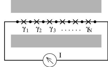
FIG. 1.: Sketch of the array geometry considered in our model. There are $N$ junctions (crosses), labeled by their gauge-invariant phase differences $\gamma_{j}$, and $N+1$ superconducting islands. A current $I$ is injected into one end of the array and extracted from the other. The array is placed in an electromagnetic cavity which supports a single resonant photon mode of frequency $\Omega$.

old for coherence and self-induced resonant steps.

In the present paper, we give a more complete derivation of the model equations of motion of Ref. [25] for a one-dimensional array of underdamped Josephson junctions coupled to a single-mode electromagnetic cavity. Starting from a suitable Hamiltonian, we obtain the Heisenberg equations of motions for the phase differences and the photon creation and annihilation operators. We account for dissipation in the junctions by the standard procedure of coupling each junction to a reservoir of phonon variables with a density of states constructed so as to produce ohmic damping. In the limit of large numbers of photons, the equations can be treated classically and solved numerically. We also correct the treatment of Ref. [25] of the junction damping and the coupling of the array to an external current. Finally, we carry out a canonical transformation of our Hamiltonian to show that the interaction between the array and the cavity mode has the form of a capacitive coupling.

We also present much more extensive numerical results than those of Ref. [25], based on solutions to the model equations. Our numerical results show all the principal features of the measurements, including SIRS’s, a coherence threshold, and a quadratic dependence of the photon energy in the cavity upon number of active junctions. Plots of the IV characteristics and other calculated features closely resemble the corresponding experimental plots. This agreement is especially noticeable since the calculation is one-dimensional, while most experiments have been conducted on two-dimensional arrays. In addition, we find that by tuning the initial conditions, we can cause the array to lock into a variety of different integer SIRS’s, again in agreement with experiment. We conclude that these equations do indeed describe the experiment, and that a one-dimensional array is sufficient to achieve this type of coherent behavior.

The remainder of this paper is organized as follows. In Section II, we derive the Heisenberg equations of motion for the phase and photon variables, starting from a model Hamiltonian. We also apply a canonical transformation which shows that the Hamiltonian involves a kind of distributed capacitive coupling between the Josephson array and the cavity mode. In Section III, we give a detailed description of our numerical results. Section IV presents a comparison between our results and experiment, gives a qualitative discussion of the numerical results, and makes some concluding remarks about the model.

II Derivation of the Equations of Motion

A Hamiltonian

We consider a one-dimensional array of N Josephson junctions placed in a resonant cavity, which we assume supports only a single photon mode of frequency $\Omega$ (the geometry is sketched in Fig. 1). The array is to be driven by an applied current $I$. We write the Hamiltonian in the form

$$H=H_{photon}+H_{J}+H_{C}+H_{curr}+H_{diss}.$$ (1)

Here, $H_{photon}$ is the energy of the cavity mode, which we express as

$$H_{photon}=\hbar\Omega\left(a^{\dagger}a+\frac{1}{2}\right),$$ (2)

with $a^{\dagger}$ and $a$ as the usual photon creation and annihilation operators. $H_{J}$ is the Josephson Hamiltonian, and is assumed to take the form

$$H_{J}=-\sum_{j=1}^{N}E_{Jj}\cos\gamma_{j},$$ (3)

where $E_{Jj}$ is the Josephson energy of the j^th junction, and $\gamma_{j}$ is the gauge-invariant phase difference across the j^th junction (defined more precisely below). $E_{Jj}$ is related to $I_{cj}$, the critical current of the j^th junction, by $E_{Jj}=\hbar I_{cj}/q$, where $q=2|e|$ is the Cooper pair charge. $H_{C}$ is the capacitive energy of the N junctions, which we approximate as

$$H_{C}=\sum_{j=1}^{N}E_{Cj}n_{j}^{2}.$$ (4)

Here, $E_{Cj}=q^{2}/(2C_{j})$ is the capacitive energy of the j^th junction, $C_{j}$ is the capacitance of that junction, and $n_{j}$ is the difference between the number of Cooper pairs on the j^th and $(\mbox{j}+1)^{th}$ superconducting island.

The gauge-invariant phase difference, $\gamma_{j}$, is the term which couples the Josephson junctions to the cavity. It may be written as

$$\gamma_{j}=\phi_{j}-[(2\pi)/\Phi_{0}]\int_{j}{\bf A}\cdot{\bf ds}\equiv~{}\phi_{j}-A_{j},$$ (5)

where $\phi_{j}$ is the phase difference across the j^th junction in a particular gauge, ${\bf A}$ is the vector potential in that same gauge, $\Phi_{0}=hc/q$ is the flux quantum, and the line integral is taken across the junction. We assume that ${\bf A}$ arises from the electromagnetic field of the normal mode of the cavity. In Gaussian units, this vector potential takes the form[28, 29]

$${\bf A}({\bf x},t)=\sqrt{(hc^{2})/(\Omega)}\left(a(t)+a^{\dagger}(t)\right){\bf E}({\bf x}),$$ (6)

where ${\bf E}({\bf x})$ is a vector proportional to the local electric field of the mode, normalized such that $\int_{V}d^{3}x|{\bf E}({\bf x})|^{2}=1$, where $V$ is the cavity volume. Given this representation for ${\bf A}$, the phase factor $A_{j}$ can be written

$$A_{j}=\sqrt{g_{j}}(a+a^{\dagger}),$$ (7)

where $g_{j}$ takes the form

$$g_{j}=\frac{\hbar c^{2}}{\Omega}\frac{(2\pi)^{3}}{\Phi_{0}^{2}}\left[\int_{j}{\bf E}({\bf x})\cdot{\bf ds}\right]^{2}.$$ (8)

Clearly, $g_{j}$ is an effective coupling constant describing the interaction between the j^th junction and the cavity[30].

The terms discussed so far need to be supplemented by the effects of a driving current and of damping within the junctions. A driving current is easily included within the Hamiltonian formalism via a “washboard potential,” H_curr, of the form

$$H_{curr}=-\frac{\hbar I}{q}\sum_{i=1}^{N}\gamma_{j},$$ (9)

with $I$ as the driving current.

The inclusion of dissipation can be done in a standard way [32, 33, 34] by coupling each gauge-invariant phase difference, $\gamma_{j}$, to a separate collection of harmonic oscillators with a suitable spectral density. Thus, we write the dissipative term in the Hamiltonian as

$$H_{diss}=\sum_{j=1}^{N}H_{diss,j},$$ (10)

where

$$H_{diss,j} = \sum_{\alpha}\left[f_{\alpha,j}~{}\gamma_{j}u_{\alpha,j}+\frac{p_{\alpha,j}^{2}}{2m_{\alpha,j}}\right.$$ (11)

$$+ \left.\frac{1}{2}~{}m_{\alpha,j}~{}\omega_{\alpha,j}^{2}~{}u_{\alpha,j}^{2}+\frac{(f_{\alpha,j})^{2}}{2m_{\alpha,j}~{}\omega_{\alpha,j}^{2}}(\gamma_{j})^{2}\right].$$ (12)

The variables $u_{\alpha,j}$ and $p_{\alpha,j}$, describing the $\alpha^{th}$ oscillator in the j^th junction, are canonically conjugate, and $m_{\alpha,j}$ and $\omega_{\alpha,j}$ are the mass and frequency of that oscillator. The last term in Eq. (12) must be added in order to prevent the original potential from being shifted by the coupling to the j^th phase degree of freedom [33]. The spectral density of the harmonic oscillators in the j^th junction, denoted $J_{j}(\omega)$, is defined by

$$J_{j}(\omega)\equiv(\frac{\pi}{2})\sum_{\alpha}\frac{(f_{\alpha,j})^{2}}{m_{\alpha}\omega_{\alpha}}~{}\delta(\omega-\omega_{\alpha}).$$ (13)

If $J_{j}(\omega)$ is linear in $|\omega|$, it can be shown that the dissipation in the junction is ohmic [32, 33, 34]. We write such a linear spectral density as

$$J_{j}(\omega)=\frac{\hbar}{2\pi}~{}\alpha_{j}~{}|\omega|~{}\Theta(\omega_{c}-\omega),$$ (14)

where $\omega_{c}$ is a high-frequency cutoff (at which the assumption of ohmic dissipation begins to break down), $\Theta(\omega_{c}-\omega)$ is the usual step function, and $\alpha_{j}$ is a dimensionless constant, which we write as $\alpha_{j}=R_{0}/R_{j}$, where $R_{0}=h/(4e^{2})$ and $R_{j}$ is a constant with dimensions of resistance (actually, the effective shunt resistance of the junction, as discussed below).

B Equations of Motion

It is now convenient to introduce the operators $a_{R}$ and $a_{I}$ by

$$a=a_{R}+ia_{I};$$ (15)

$$a^{\dagger}=a_{R}-ia_{I}.$$ (16)

The free photon part of the Hamiltonian can be expressed in terms of $a_{R}$ and $a_{I}$ as follows:

$$H_{photon}=\hbar\Omega(a_{R}^{2}+a_{I}^{2}),$$ (17)

where we have used the additional commutation relations $[a_{R},a_{I}]=i/2$, which follows from the usual relation $[a,a^{\dagger}]=1$. The gauge-invariant phase difference, $\gamma_{j}$, is related to $\phi_{j}$ by

$$\gamma_{j}=\phi_{j}-2\sqrt{g_{j}}a_{R}.$$ (18)

The time-dependence of the various operators appearing in the Hamiltonian (1) is now obtained from the Heisenberg equations of motion. For a general operator ${\cal O}$, these take the form

$$\dot{{\cal O}}=\frac{1}{i\hbar}[{\cal O},H].$$ (19)

These equations of motion can be evaluated for the various operators entering $H$, using the commutation relation $[A,F(B)]=[A,B]F^{\prime}(B)$, where $F$ is any function of an operator B, and $F^{\prime}(B)$ is the derivative of that function. One also needs the commutation relations for the various operators in the Hamiltonian (1). Besides the relations already given, these are as follows:

$${[}n_{j},\gamma_{k}{]} = -i\delta_{jk};$$ (20)

$${[}p_{\alpha,j},u_{\beta,k}{]} = -i\hbar~{}\delta_{\alpha,\beta}~{}\delta_{j,k}.$$ (21)

Note that $\gamma_{k}$, unlike $\phi_{j}$, no longer commutes with $a_{I}$; instead, it satisfies

$${[}\gamma_{j},a_{R}{]} = 0;$$ (22)

$${[}\gamma_{j},a_{I}{]} = -i\sqrt{g_{j}}.$$ (23)

Using all these relations, we find, after a little algebra, the following equations of motion for the operators $\gamma_{j}$, $n_{j}$, $a_{R}$, and $a_{I}$:

$$\dot{\gamma}_{j} = 2~{}\frac{E_{Cj}}{\hbar}~{}n_{j}-2~{}\Omega~{}\sqrt{g_{j}}~{}a_{I},$$ (24)

$$\dot{n}_{j} = -\frac{E_{Jj}}{\hbar}\sin(\gamma_{j})+\frac{I}{q}$$ (26)

$$-\frac{1}{\hbar}\sum_{\alpha}\left(f_{\alpha,j}~{}u_{\alpha,j}+\frac{(f_{\alpha,j})^{2}}{m_{\alpha,j}\omega_{\alpha,j}^{2}}~{}\gamma_{j}\right),$$

$$\dot{a}_{R} = \Omega~{}a_{I},$$ (27)

$$\dot{a}_{I} = -\Omega~{}a_{R}+\sum_{j}\sqrt{g_{j}}~{}\frac{E_{Jj}}{\hbar}~{}\sin(\gamma_{j})-\frac{I}{q}\sum_{j}\sqrt{g_{j}}$$ (29)

$$+\sum_{j}\frac{\sqrt{g_{j}}}{\hbar}~{}\sum_{\alpha}\left(f_{\alpha,j}~{}u_{\alpha,j}+\frac{(f_{\alpha,j})^{2}}{m_{\alpha,j}\omega_{\alpha,j}^{2}}~{}\gamma_{j}\right).$$

These are equations of motion for the operators $a_{R}$, $a_{I}$, $n_{j}$, and $\phi_{j}$ (or $\gamma_{j}$). Note that they do not depend on the particular choice of gauge, but only on the form of the Hamiltonian and the commutation relations for the various operators. We will study these general equations within the limit of large number of photons in the cavity and large number of charges in the junctions, and in this “classical” limit, we will regard the operators as $c$-numbers [31].

We also have the equations of motion for the harmonic oscillator variables. Since we have no explicit interest in these variables for themselves, we instead eliminate them in order to incorporate the dissipative term into the equations of motion. Such a replacement is possible provided that the spectral density of each junction is linear in frequency, as noted above. In that case [32, 33, 34], the oscillator variables can be integrated out. The effect of carrying out this procedure is that one should make the replacement

$$\sum_{\alpha}\left(f_{\alpha,j}~{}u_{\alpha,j}+\frac{(f_{\alpha,j})^{2}}{m_{\alpha,j}\omega_{\alpha,j}^{2}}~{}\gamma_{j}\right)\rightarrow\frac{\hbar}{2\pi}\frac{R_{0}}{R_{j}}~{}\dot{\gamma}_{j}$$ (30)

wherever this sum appears in the equations of motion.

Making the replacement (30) in Eqs. (26) and (29), we obtain the equations of motion for $n_{j}$ and $a_{I}$ with damping:

$$\dot{n}_{j} = -\frac{E_{Jj}}{\hbar}\sin(\gamma_{j})+\frac{I}{q}-\frac{\bar{\omega}_{p}}{2\omega_{Cj}Q_{Jj}}~{}\dot{\gamma}_{j}$$ (31)

$$\dot{a}_{I} = -\Omega~{}a_{R}+\sum_{j}\sqrt{g_{j}}~{}\frac{E_{Jj}}{\hbar}~{}\sin(\gamma_{j})$$ (33)

$$-\frac{I}{q}\sum_{j}\sqrt{g_{j}}+\sum_{j}\sqrt{g_{j}}~{}\frac{\bar{\omega}_{p}}{2\omega_{Cj}Q_{Jj}}~{}\dot{\gamma_{j}}.$$

Here, we have introduced the parameters $\omega_{Cj}=E_{Cj}/\hbar$, which is a frequency associated with the capacitive energy of the j^th junction; $\bar{\omega}_{p}=\frac{1}{N}\sum_{j=1}^{N}\omega_{pj}$, the average of the Josephson plasma frequencies $\omega_{pj}=\sqrt{2E_{Cj}E_{Jj}}/\hbar$; and $Q_{Jj}$, the dimensionless junction quality factor (or damping parameter) for the j^th junction, which is related to the capacitance $C_{j}$ and the shunt resistance $R_{j}$ by

$$Q_{Jj}=\bar{\omega}_{p}R_{j}C_{j}.$$ (34)

Eqs. (24), (27), (31), and (33) can be combined, with a little algebra, into two coupled second-order differential equations:

$$\frac{1}{2\omega_{Cj}}~{}\ddot{\gamma}_{j}+\frac{\bar{\omega}_{p}}{2\omega_{Cj}Q_{Jj}}~{}\dot{\gamma}_{j} + \omega_{Jj}~{}\sin\gamma_{j}$$ (35)

$$= \frac{I}{q}-\frac{\sqrt{g_{j}}}{\omega_{Cj}}~{}\ddot{a}_{R}$$ (36)

and

$$\left(1+\Omega\sum_{j}\frac{g_{j}}{\omega_{Cj}}\right)\ddot{a}_{R}+\Omega^{2}~{}a_{R}=-\frac{\Omega}{2}~{}\sum_{j}\frac{\sqrt{g_{j}}}{\omega_{Cj}}~{}\ddot{\gamma}_{j}.$$ (37)

where we have defined $\omega_{Jj}=E_{Jj}/\hbar$. Note that in the absence of coupling between the junctions and the cavity, $\gamma_{j}=\phi_{j}$, Eq. (36) reduces to the usual equation of motion for a resistively and capacitively shunted junction[35] driven by a current $I$, and Eq. (37) reduces to that of a simple harmonic oscillator which represents the cavity mode. Note that we have not included any damping due to the cavity walls. While such damping is undoubtedly present, we find that good agreement with experiment can be obtained without including it.

C Canonical Transformation

The physics behind the coupling between the Josephson junctions and the resonant cavity, and hence the physics of Eqs. (24) - (29), can be made clearer by a canonical transformation. For simplicity, we describe this transformation including only the terms H_phot, H_J, and $H_{C}$ from the Hamiltonian (1), and omitting $H_{curr}$ and $H_{diss}$. The same transformation has previously been used for a single junction coupled to a resonant cavity by Buisson and Hekking[36]; and, for two voltage-driven junctions coupled to a resonant cavity, by Shnirman et al [37].

We begin by writing

$$H^{\prime} \equiv H_{phot}+H_{J}+H_{C}~{}=~{}\frac{1}{2}\hbar~{}\Omega~{}(p_{r}^{2}+q_{r}^{2})$$ (39)

$$~{}+~{}\sum_{j=1}^{N}\bigg{[}E_{Cj}n_{j}^{2}-E_{Jj}\cos(\phi_{j}-\sqrt{2g_{j}}~{}q_{r})\bigg{]},$$

where we have defined $p_{r}=\sqrt{2}~{}a_{I}$ and $q_{r}=\sqrt{2}~{}a_{R}$. With this choice, $p_{r}$ and $q_{r}$ satisfy the commutation relation $[p_{r},q_{r}]=-i$. Next, we make the canonical transformation

$$n^{\prime}_{j} = n_{j};$$ (40)

$$\phi^{\prime}_{j} = \phi_{j}-\sqrt{2g_{j}}~{}q_{r};$$ (41)

$$p^{\prime}_{r} = p_{r}+\sum_{j=1}^{N}\sqrt{2g_{j}}~{}n_{j};$$ (42)

$$q^{\prime}_{r} = q_{r}.$$ (43)

The only nonvanishing commutators of the primed variables are easily shown to be $[n^{\prime}_{j},\phi^{\prime}_{j}]=[p^{\prime}_{r},q^{\prime}_{r}]=-i$. Re-expressing the Hamiltonian (39) in terms of the primed variables, we obtain

$$H^{\prime} = \frac{1}{2}\hbar\Omega\left(p^{\prime}_{r}-\sum_{j}\sqrt{2g_{j}}n_{j}^{\prime}\right)^{2}+\frac{1}{2}\hbar\Omega(q^{\prime}_{r})^{2}$$ (45)

$$+~{}\sum_{j=1}^{N}\bigg{[}E_{Cj}(n^{\prime}_{j})^{2}-E_{Jj}\cos\phi^{\prime}_{j}\bigg{]}$$

Thus, $H^{\prime}$ is the sum of four terms: the sum $(\hbar\Omega/2)[(p_{r}^{\prime})^{2}+(q_{r}^{\prime})^{2}]$ describes the cavity resonator; the last sum describes the $N$ independent junctions; and the remaining terms represent the interaction between the junctions and the resonator, and an indirect interaction between the junction variables $n_{j}^{\prime}$ mediated by the cavity.

To interpret this interaction, we note that the junction-cavity system has two places in which charge can be stored: the variables $n_{j}^{\prime}$ of the junctions and the variables $p_{r}^{\prime}$ of the cavity. The cavity behaves much like an $LC$ circuit, with capacitive energy $(\hbar\Omega/2)(p_{r}^{\prime})^{2}$ and inductive energy $(\hbar\Omega/2)(q_{r}^{\prime})^{2}$. The dominant interaction is a capacitive coupling between the charge variables $n_{j}^{\prime}$ of the junction and the charge variable $p_{r}^{\prime}$ of the cavity[38].

In further support of this interpretation, we now show that $H^{\prime}$, in the form (45), is equivalent to that given by Shnirman et al [37] in the case of zero applied voltage. Fig. 1 of Ref. [35] depicts each junction contained between the plates of a capacitor with capacitance $C$. The junction itself has capacitance $C_{J}$. The system of junction and capacitor is then shunted by a parallel inductance, $L$, which acts to couple all the junctions together [39]. The equivalence is established by noting the correspondence between the variables used in the present paper and the variables $\phi$, $q$, $n_{j}$ and $\theta_{j}$ of Ref. [35]. The correspondence is as follows (assuming that the coupling constants $g_{j}$, $E_{Cj}$, and $E_{Jj}$ are independent of $j$):

$$q_{r}^{\prime} \leftrightarrow [L/(2C_{t})]^{-1/4}\phi;$$ (46)

$$p_{r}^{\prime} \leftrightarrow [L/(2C_{t})]^{1/4}q;$$ (47)

$$n_{j}^{\prime} \leftrightarrow n_{j}$$ (48)

$$\phi_{j}^{\prime} \leftrightarrow \theta_{j},$$ (49)

where $C_{t}=CC_{J}/(C+2C_{J})$. In order to complete the correspondence, we also give the correspondence between the remaining parameters and the quantities $L$, $C$, $C_{t}$,and $C_{J}$:

$$\sqrt{2g} = \left(\frac{L}{2C_{t}}\right)^{1/4}\frac{C_{t}}{C_{J}};$$ (50)

$$\Omega = \frac{1}{\sqrt{2LC_{t}}};$$ (51)

$$E_{C} = \frac{1}{C+2C_{J}},$$ (52)

If we make the replacements and identifications given above, then our Hamiltonian, for the case of two junctions, is identical to that considered in [35] in the absence of an applied voltage. The main differences between the two models are the boundary conditions: constant current bias in our model, and fixed voltage bias in that of Ref. [35].

D Dimensionless Form

In order to write these equations of motion in a simpler form, we now introduce the dimensionless time $\tau=\bar{\omega}_{p}t$. Also, although we allow disorder in the parameters of the different Josephson junctions, we assume that the coupling constants between the junctions and the cavity are all the same, i. e., that $g_{j}=g$ for all $j$. In addition, for simplicity, we assume that the products $R_{j}C_{j}$ and $I_{cj}/C_{j}$, and hence $\omega_{pj}$, are independent of $j$. Then $Q_{Jj}$ is also $j$-independent, and we may introduce the dimensionless coupling constant

$$\tilde{g}=g~{}\frac{E_{J}}{\hbar\bar{\omega}_{p}},$$ (53)

which is also independent of $j$. Similarly, we introduce a scaled number variable $\tilde{n}_{j}$ by

$$\tilde{n}_{j}=\frac{2E_{Cj}}{\hbar\bar{\omega}_{p}}~{}n_{j},$$ (54)

a dimensionless frequency $\tilde{\Omega}$ by $\tilde{\Omega}=\Omega/\bar{\omega}_{p}$, and scaled photon variables $\tilde{a}_{R}$ and $\tilde{a}_{I}$ by

$$\tilde{a}_{R} = \sqrt{g}~{}a_{R};$$ (55)

$$\tilde{a}_{I} = \sqrt{g}~{}a_{I}.$$ (56)

Finally, we assume that the critical currents $I_{cj}$ are random and uniformly distributed between $I_{c}(1-\Delta)$ and

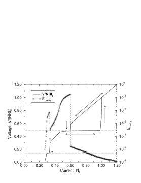
FIG. 2.: Left-hand scale and solid line: current-voltage (IV) characteristics of a one dimensional array of $N=40$ junctions, with disorder parameter $\Delta=0.05$ and coupling constant $\tilde{g}=0.001$. The resonant frequency of the cavity is $\tilde{\Omega}=2.2$, and the damping parameter of the junctions is $Q_{J}=\sqrt{20}$. Right-hand scale and stars : scaled total energy $\tilde{E}=gE/(\hbar\Omega)$ carried by the resonant mode of the cavity, plotted as a function of decreasing current $I/I_{c}$. The vertical dashed lines are guides to the eye. The upper dashed horizontal line indicate the expected position of the integer self-induced resonant steps (SIRS’s) for the particular resonant frequency $\tilde{\Omega}$ of the cavity (all junctions in the $n=1$ SIRS). For the lower dashed horizontal line, 23 junctions are on the $n=1/2$ SIRS, and 17 junctions are in the $\langle V_{j}\rangle_{\tau}=0$ state. Branches corresponding to increasing and decreasing current are shown by arrows. Double-headed arrows on this and subsequent Figures denote that the curve can be obtained by sweeping the current in either direction.

$I_{c}(1+\Delta)$, where $\Delta$ is a measure of the degree of disorder. After some algebra, we eventually obtain the following equations of motion:

$$\dot{\gamma}_{j} = \tilde{n}_{j}-2~{}\tilde{\Omega}~{}\tilde{a}_{I};$$ (57)

$$\dot{\tilde{n}}_{j} = \frac{I}{I_{c}(1+\Delta_{j})}-\frac{\tilde{n}_{j}}{Q_{J}}-\sin(\gamma_{j})+2~{}\frac{\tilde{\Omega}}{Q_{J}}~{}\tilde{a}_{I};$$ (58)

$$\dot{\tilde{a}}_{R} = \tilde{\Omega}~{}\tilde{a}_{I};$$ (59)

$$\dot{\tilde{a}}_{I} = -\tilde{\Omega}~{}\tilde{a}_{R}-2~{}\tilde{\Omega}~{}\tilde{g}~{}\frac{\tilde{a}_{I}}{Q_{J}}~{}\sum_{j}(1+\Delta_{j})-N~{}\tilde{g}~{}\frac{I}{I_{c}}$$ (60)

$$+ \tilde{g}~{}\sum_{j}(1+\Delta_{j})\sin(\gamma_{j})+\frac{\tilde{g}}{Q_{J}}~{}\sum_{j}(1+\Delta_{j})~{}\tilde{n}_{j}.$$ (61)

In these equations, the dot refers to differentiation with respect to $\tau$, and the j^th critical current is $I_{c}(1+\Delta_{j})$.

These equations can be combined into two more compact equations, with the result

$$\ddot{\gamma}_{j}+\frac{1}{Q_{J}}~{}\dot{\gamma}_{j}+\sin(\gamma_{j}) = \frac{I}{I_{c}(1+\Delta_{j})}-2~{}\ddot{\tilde{a}}_{R};$$ (62)

$$\ddot{\tilde{a}}_{R}+(\Omega^{\prime})^{2}~{}\tilde{a}_{R} = -\tilde{g}~{}\frac{\Omega^{\prime}}{\tilde{\Omega}}~{}\sum_{j=1}^{N}(1+\Delta_{j})~{}\ddot{\gamma}_{j},$$ (63)

where we have defined $(\Omega^{\prime})^{2}~{}=~{}\tilde{\Omega}^{2}/[1+2~{}\tilde{g}~{}\tilde{\Omega}\sum_{j}(1+\Delta_{j})]$. Eqs. (62) and (63) are the analogs of Eqs. (36) and (37), expressed in terms of dimensionless reduced variables.

III Numerical Results

We have solved Eqs. (62) and (63) for the variables $\tilde{n}_{j}$, $\gamma_{j}$, $\tilde{a}_{R}$ and $\tilde{a}_{I}$ numerically using the same approach as in Ref. [25], namely, by implementing the rapid and accurate adaptive Bulrisch-Stoer method [40]. We initialize the simulations with all the phases randomized between $[0,2\pi]$, and usually $\tilde{a}_{R}=\tilde{a}_{I}=\tilde{n}_{j}=0$. We then let the system equilibrate for a time interval $\Delta\tau=10^{4}$, after which we evaluate averages over a time interval $\Delta\tau=2\cdot 10^{3}$, using $2^{16}$ evenly spaced sampling points.

A Typical IV Characteristics, Power Spectrum, and Coherence Transition

In Fig. 2, we show a representative current-voltage (IV) characteristic calculated for an array of $N=40$ junctions with $\Delta=0.05$ and $\tilde{g}=0.001$. The time-averaged voltage $\langle V\rangle_{\tau}$ [left-hand scale] is obtained from

$$\langle V\rangle_{\tau}=\sum_{j=1}^{N}\langle V_{j}\rangle_{\tau},$$ (64)

where $\langle...\rangle_{\tau}$ denotes a time average and $V_{j}$ is obtained from the Josephson relation,

$$\frac{V_{j}}{RI_{c}}=\frac{\hbar}{qRI_{c}}\frac{d\gamma_{j}}{dt}=\frac{1}{Q_{J}}~{}\dot{\gamma}_{j}.$$ (65)

A striking feature of this plot is the self-induced resonant steps (SIRS), at which $\langle V\rangle_{\tau}$ remains approximately constant over a range of applied current. For this particular choice of parameters and initial conditions, we see these steps at $\langle V\rangle_{\tau}/(NRI_{c})=n\tilde{\Omega}/Q_{J}$. These steps corresponds to voltages at which the condition

$$2e\langle V_{j}\rangle_{t}=n\hbar\Omega$$ (66)

is satisfied for the individual junctions, with $n=1$ (upper horizontal dashed line) and $n=1/2$ (lower horizontal dashed line). Thus, the lower step is at 23/80 the voltage of the upper step. For the latter case, the driving current is smaller than the retrapping currents of $17$ of the junctions; thus, only $23$ out of the $40$ junctions are oscillating on this step. (The retrapping current is the minimum current for which an underdamped junction is bistable.) The steps occur at exactly the voltages where the first integer and half-integer steps would appear in

FIG. 3.: Power spectrum, $P(\omega)$ (Eq. 68), of the a. c. voltage across the array, plotted versus frequency, $\tilde{\Omega}$, at two driving currents: (a) and (b) $I/I_{c}=0.58$, corresponding to the first integer SIRS, and (c) and (d) $I/I_{c}=0.65$, slightly off a SIRS. Other parameters are the same as in Fig. 2. Panels (b) and (d) are the same as (a) and (c) except that the effective coupling to the resonant cavity, $\tilde{g}=0$. In each panel, the left vertical dashed line shows the resonant frequency of the cavity, and the right vertical, dashed line shows the average resonant frequency of the junctions for the case of no coupling to the cavity.

these junctions, if the junctions were driven by an a. c. current of frequency $\tilde{\Omega}$. Thus, the radiated energy in the cavity seems to behave like an a. c. drive which acts back to induce these steps in the junctions of the array. Similar steps were seen experimentally in a two-dimensional array of underdamped Josephson junctions coupled to a resonant cavity [19], and in more recent experiments in 1D arrays [41].

Fig. 2 also shows the time-averaged scaled total energy, $\tilde{E}$, contained in the cavity, [right-hand scale of the Figure]. $\tilde{E}$ is defined as

$$\tilde{E}=\langle\tilde{a}_{R}^{2}+\tilde{a}_{I}^{2}\rangle_{\tau}=g~{}\langle a_{R}^{2}+a_{I}^{2}\rangle_{\tau}=\frac{g}{\hbar\Omega}E,$$ (67)

where $E=\langle H_{photon}\rangle_{\tau}$ is the cavity energy; it is plotted as a function of $I/I_{c}$ for the same array. As is evident, $\tilde{E}$ increases dramatically when the array is on a SIRS, and is very small otherwise. This sharp increase signals the onset of coherence within the array, and can be qualitatively understood from the equations of motion. Specifically, when the array sits on one of the integer SIRS, all the junctions are oscillating in phase. Hence, the term driving $\tilde{a}_{R}$ [the right-hand side of Eq. (63)], and thus $\tilde{a}_{R}$ itself, are both proportional to the number $N_{a}$ of active junctions.

Before proceeding further, we briefly review the concept of active junction number $N_{a}$, as discussed in Refs. [12] and [25]. This concept has meaning only for underdamped junctions. Such a junction is bistable and hysteretic in certain ranges of current - that is, it can have either zero or a finite time-averaged voltage across it, depending on the initial conditions. In the present case, $N_{a}$ denotes the number of junctions (out of $N$ total) which have a finite time-averaged voltage drop. It is possible to tune $N_{a}$ by suitably choosing the initial conditions, $\gamma_{i}$ and $\dot{\gamma}_{i}$, in simulations[14, 27].

Fig. 3 shows the calculated voltage power spectrum of the a. c. component of the total voltage across the array

$$P(\omega)=2~{}\lim_{T\rightarrow\infty}\left|\frac{1}{T}\int_{0}^{T}V(\tau)~{}e^{i\omega\tau}d\tau\right|^{2},$$ (68)

for two values of the driving current: $I/I_{c}=0.58$ [Fig. 3(a) and (b)] and $I/I_{c}=0.65$ [Fig. 3(c) and (d)]; all other parameters are the same as in Fig. 2. In (a), all the junctions are on the first SIRS, while in (c), the array is tuned off this step. In Fig. 3(b) and 3(d), we show the same case as in Fig. 3(a) and (c) respectively, except that the coupling constant, $\tilde{g}$, is artificially set equal to zero. Note that in 3(a), the power spectrum has peaks at the scaled cavity frequency, $\tilde{\Omega}$, and its harmonics. This is evidence that the junctions are all oscillating at frequency $\tilde{\Omega}$. In case (b), the junctions are still coupled by the indirect interaction via the cavity, but the power spectrum shows that the array is not synchronized in this case; instead, the individual junctions oscillate approximately at their individual resonant frequencies and their harmonics and subharmonics. Hence, the power spectrum has a spread of frequencies, all of which differ from that of the cavity. In cases (b) and (d), the junctions are, of course, independent of one another, and the power spectrum is that of a disordered one-dimensional Josephson array with no coupling between the junctions.

We have also calculated the response of a disordered array ($\Delta=0.05$) of fixed length ($N=40$ junctions), and a driving current $I/I_{c}=0.58$, when the number of active junctions, $N_{a}$ is varied. This current not only lies well within the bistable region, but also leads to a voltage on the first integer SIRS. In Fig. 4(a), we plot the time-averaged scaled energy of the cavity, $\tilde{E}(N_{a})$ [Eq. (67)], as a function of $N_{a}$. For $N_{a}<17$, the active junctions are unsynchronized, and $\tilde{E}$ is correspondingly small and only weakly dependent on $N_{a}$. There is a sudden jump in $\tilde{E}$ at a critical number of active junctions $N_{c}=17$. Above this value $\tilde{E}$ increases as a quadratic function of $N_{a}$, and we have fitted $\tilde{E}(N_{a})$ to the form $\tilde{E}=c_{0}+c_{1}N_{a}+c_{2}N_{a}^{2}$. The constants which give the best fit are $c_{0}=-0.00163$; $c_{1}=0.00125$; and $c_{2}=6.868\cdot 10^{-5}$. This curve is shown as a full line in Fig. 4(a); the fit is clearly excellent. As a contrast, we also show the best linear fit to the same data set (dashed line); the fit is plainly less good. The magnitude of the jump in $\tilde{E}$ at $N_{a}=N_{c}$ is nearly a factor of $\sim 10^{3}$, as shown in the inset to figure.

To measure the degree of synchronization among the Josephson junctions, we have also calculated the Kuramoto order parameter [42], $\langle r\rangle_{\tau}$, for the same parameters,

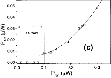
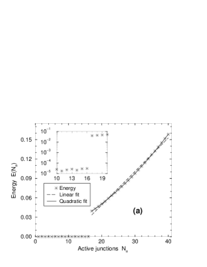
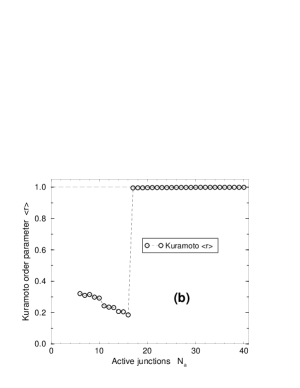
FIG. 4.: (a) Asterisks: Scaled photon energy $\tilde{E}=gE/(\hbar\Omega)$ in the resonant cavity when the array is current driven on a SIRS, plotted versus number of active junctions, $N_{a}$. The array parameters are $N=40$, $\tilde{\Omega}=2.2$, $Q_{J}=\sqrt{20}$, $\Delta=0.05$, $\tilde{g}=0.001$, and $I/I_{c}=0.58$ [cf. Fig. 3 (a)]. Full curve shows the best fit of $\tilde{E}$ to the function $c_{2}N_{a}^{2}+c_{1}N_{a}+c_{0}$ for $N_{a}>17$, the threshold for synchronization. The fitting parameters are $c_{0}=-0.00163$, $c_{1}=0.00125$, and $c_{2}=6.868\cdot 10^{-5}$. We contrast this fit to the best linear fit (dashed line). Inset: $\tilde{E}(N_{a})$ near $N_{c}=17$, showing jump near synchronization threshold. (b) Open circles: Kuramoto order parameter, $\langle r\rangle_{\tau}$ [Eq. (69)], for the same array. Dots connecting circles are guides to the eye. The sharp increase in $\langle r\rangle_{\tau}$ and the quadratic increase in $\tilde{E}$ both begin at $N_{c}=17$. (c) Measured a. c. power as a function of the input d. c. power, as obtained in Ref. [17] for a $3\times 36$ array. The d. c. power is proportional to the number of active rows in their array, while the a. c. power is proportional to the energy $\tilde{E}$ in the cavity.

as a function of number of active junctions, $N_{a}$. $\langle r\rangle_{\tau}$ is defined by

$$\langle r\rangle_{\tau}=\langle|\frac{1}{N_{a}}\sum_{j=1}^{N_{a}}\exp(i\gamma_{j})|\rangle_{\tau}.$$ (69)

The results are shown in Fig. 4(b). Note that $\langle r\rangle_{\tau}=1$ represents perfect synchronization among the active junctions, while $\langle r\rangle_{\tau}=0$ would correspond to no correlations between the different phase differences, $\phi_{i}$. Just as for $\tilde{E}(N_{a})$, there is an abrupt increase in $\langle r\rangle_{\tau}$ at $N_{a}=N_{c}$, indicative of a dynamical transition from an unsynchronized to a synchronized state (with all active junctions locked to the same frequency and having a common phase), as $N_{a}$ is increased keeping all other parame-

ters fixed. As with similar transitions in other models [43], this transition is not inhibited by the finite disorder in the $I_{c}$’s. Instead, $\langle r\rangle_{\tau}$ approaches unity, representing perfect synchronization. $\langle r\rangle_{\tau}$ remains finite even for $N_{a}<N_{c}$, because even in this regime there is still some residual correlation among the phases in different active junctions. This transition is the dynamic analog of that analyzed by an equilibrium mean-field theory in Ref. [24].

Finally, in Fig. 4(c), we show an experimental plot of the detected a. c. power as a function of the input d. c. power, as measured by Barbara et al[19] for a $3\times 36$ array. These quantities are, of course, not equivalent to the calculated results which are plotted in Fig. 4 (a). The input d. c. power is equal to the power dissipated in the active junctions; so it is proportional to $N_{a}$. The detec-

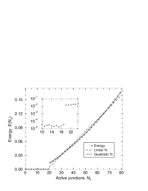
FIG. 5.: Same as Fig. 4(a), except that $N=80$. In this case, the synchronization threshold is $N_{c}=20$, and the quadratic fit to the energy above synchronization has different fitting parameters: $c_{0}=-0.01576$, $c_{1}=0.001149$, and $c_{2}=1.441\cdot 10^{-5}$.

ted a. c. power is that measured by a pickup junction in the cavity, and thus should be proportional to $\tilde{E}(N_{a})$ in our notation. Despite the differences, our calculated plot (for a one-dimensional array) appears strikingly similar to their measured plot, especially as regards the discontinuity at the threshold and the quadratic dependence on $N_{a}$ for $N_{a}$ above the threshold.

In Fig. 5, we show the synchronization transition for an array of $N=80$ junctions, keeping the other parameters the same as in Fig. 4(a). In this case, the critical threshold is $N_{c}=20$, somewhat larger than for the $N=40$ junction array. The inset shows that the cavity energy still has a discontinuity by a factor of $\sim 10^{3}$. However, the quadratic function which best fits $\tilde{E}(N_{a})$ for $N_{a}\geq N_{c}$ is now described by the different fitting parameters: $c_{0}=-0.01576$, $c_{1}=0.001149$, and $c_{2}=1.441\cdot 10^{-5}$. Thus, the total length of the array alters the details but not the qualitative features of $\tilde{E}(N_{a})$.

These calculations were carried out for an array tuned to the first SIRS. If, instead, we carry out the same calculation when the array is tuned to the bistable region but not tuned to a SIRS, we find that $\tilde{E}$ does not increase quadratically with $N_{a}$. Instead, $\tilde{E}(N_{a})$ shows no threshold behavior, and, indeed, varies little with $N_{a}$. A plot of $E(N_{a})$ in this case is shown in Fig. 6. The parameters are the same as for the calculation in Fig. 4(a), except that the driving current in this case is $I/I_{c}=0.65$, which is not on a SIRS [cf. Figs. 2 and 3 ].

B Effects of Varying the Number of Active Junctions

In Fig. 7(a), we show a series of IV characteristics for a 10-junction array ($N=10$), calculated by varying the

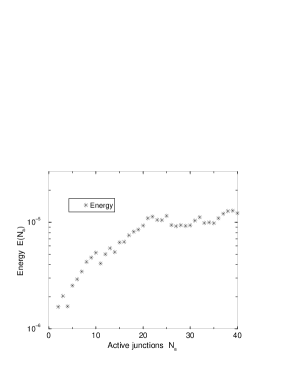
FIG. 6.: Total scaled cavity energy $\tilde{E}$ as a function of the number $N_{a}$ of active junctions, for the same array parameters as in Fig. 4(a) except that the current is tuned off any self-induced resonant step: $I/I_{c}=0.65$ [cf. Fig. 3(c)]. In this case, $\tilde{E}$ does not increase quadratically with $N_{a}$ above a critical threshold; instead, it shows no threshold behavior, is only weakly dependent on $N_{a}$, and is much smaller than in Fig. 4(a).

number $N_{a}$ of active junctions from $1$ to $10$. Each solid vertical line segment corresponds to the IV characteristic for a different $N_{a}$, and represents $N_{a}$ junctions sitting on the first integer SIRS. The width of each segment represent the current height for that step, as found in our calculation. The dashed vertical lines show the expected voltages for the integer SIRS’s, and are good matches for the calculated voltages for the various $N_{a}$’s. The long straight diagonal line segment, which is common to all the different $N_{a}$’s, represents the ohmic part of the IV characteristic with all junctions active. The nearly horizontal dashed line in the upper right hand corner of the Figure shows the IV characteristic for increasing voltage with $N_{a}=10$. The very short vertical segments within this dashed line correspond to several junctions which have been excited to higher steps, specifically the $n=2$ (second integer step) while the remaining junctions are on the $n=1$ step. The horizontal dashed line on the lower left represents the low-voltage end of the $N_{a}=10$ IV characteristic (on decreasing current). The short vertical segment within this dashed line corresponds to fractional SIRS’s – specifically, three of the junctions have slipped from the $n=1$ to the $n=1/2$ step, while the rest are in the $\langle V_{j}\rangle_{\tau}=0$ state (the driving current is smaller than their individual retrapping currents). Thus, we see both the higher integer and the fractional SIRS’s in these one-dimensional arrays.

In Fig. 7(a), although we show the full hysteresis loop only for $N_{a}=10$, the IV curves for other values of $N_{a}$ are also hysteretic. In all cases for which $N_{c}\leq N_{a}<10$, the number of active junctions increases when the SIRS becomes unstable, and individual junctions jump into the

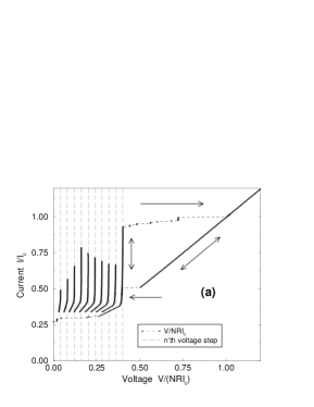
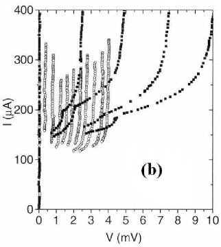
FIG. 7.: (a) Current $I/I_{c}$ versus time-averaged voltage $\langle V\rangle_{\tau}/(NRI_{c})$ for an array containing $N=10$ junctions, and with damping parameter $Q_{J}=\sqrt{20}$, disorder $\Delta=0.05$, cavity coupling $\tilde{g}=0.003$, and cavity resonance frequency of $\tilde{\Omega}=1.8$. By properly choosing the initial conditions, one can select the number $N_{a}$ of active junctions to be any integer between $0$ and $10$. Each vertical line segment corresponds to a portion of the $IV$ characteristic for a particular choice of $N_{a}$, as obtained with increasing current (although the same result would be obtained with decreasing current). The ohmic (straight diagonal line) segment is found for $N_{a}=10$ with decreasing current. The dashed vertical lines indicate the voltages of the expected integer SIRS’s. The dashed, nearly horizontal line corresponds to increasing the voltage on the $N_{a}=10$ IV characteristic; the dots and very short vertical line segments within this dashed line corresponds to currents at which several of the active junctions jump to the $n=2$ SIRS. The short, nearly horizontal dashed line in the lower left-hand corner occurs on the decreasing current branch with $10$ active junctions. The very short vertical line segments within this dashed region correspond to several active junctions synchronizing on the $n=1/2$ SIRS, while the remainder are in the state of $\langle V_{j}\rangle_{\tau}=0$. (b). Measured IV characteristics for a $3\times 36$ array [19]. The open circles represent self-induced resonant steps corresponding to different numbers of active rows. Full squares are believed to be examples of resistance steps[44].

$n=2$ SIRS state; ohmic behavior is not attained until $I/I_{c}>1$. For $N_{a}<N_{c}$, the array behaves somewhat differently: when the SIRS becomes unstable, $N_{a}$ is unchanged, and the IV curve immediately becomes ohmic. When $I/I_{c}\sim 1$ in this regime, the remaining junctions become active and the IV characteristic also becomes ohmic. For this particular array, $N_{c}=4$.

As a comparison, we also show, in Fig. 7(b), the IV characteristics as measured for a $3\times 36$ underdamped array, by Barbara et al[19]. The open circles correspond to the steps observed for different numbers of active rows (from $1$ to $10$ in this instance), which are produced when an in-plane magnetic field reduces the critical current of the individual junctions. The more widely spaced dark rows are believed to be examples of resistance steps [44]. The steps (open circles) very much resemble those of Fig. 7(a), even including the low-current falloff (though the shapes of the curves are slightly different).

We have also calculated $\tilde{E}$, the energy in the cavity, as a function of injected d. c. power, $P_{dc}$, when the array is biased on a SIRS, for several choices of array parameters. A typical example of our results is shown in Fig. 8(a), where $\tilde{E}$ is plotted versus $P_{dc}\equiv(I/I_{c})[\langle V\rangle_{\tau}/(NRI_{c})]$ for an array of ten junctions, using the same parameters as in Fig. 7(a) and varying the values of $N_{a}$. Each curve corresponds to a different number $N_{a}$ of active junctions, and, for each $N_{a}$, we sweep current across the $n=1$ SIRS

(leftmost curve corresponds to $N_{a}=1$, and rightmost to $N_{a}=10$). The curves end when the SIRS’s become unstable. Each curve is quadratic at low $P_{dc}$ and approximately linear at higher $P_{dc}$. For comparison we also show the corresponding experimental plots [45] for a $4\times 36$ array for $N_{a}=16$, $21$, and $23$ active rows [Fig. 8(b)]. In all cases the experimental array is above $N_{c}$, the coherence threshold. The similarity between the experimental and calculated curves is strikingly apparent.

C Effects of Changing Model Parameters

Finally, we have studied how our numerical results depend on the parameters of our model. There are several parameters of interest: the number of junctions $N$, the disorder parameter $\Delta$, the damping parameter $Q_{J}$, the coupling constant $\tilde{g}$, and the normalized cavity mode frequency $\tilde{\Omega}$. Clearly, a thorough numerical investigation of all these parameters is out of the question. We have therefore varied only two parameters in the present paper: $Q_{J}$ and $\tilde{g}$.

Fig. 9 shows the total time-average voltage $\langle V\rangle_{\tau}$ across the array, and the total time-averaged energy $\tilde{E}$ in the array as a function of driving current $I/I_{c}$, for $Q_{J}=\sqrt{100}$, $\sqrt{20}$, $\sqrt{2}$, $\sqrt{0.1}$, and $\sqrt{0.05}$, all for $\tilde{g}=4\times 10^{-4}$, $N=10$, and $\Delta=0.05$. In each case, the resonant frequency of

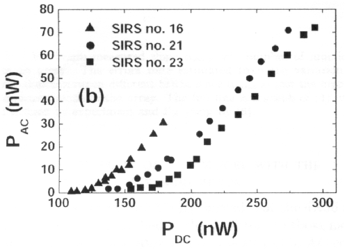
FIG. 8.: (a) Calculated total energy $\tilde{E}$ within the cavity, plotted versus d. c. power, $P_{dc}$, for $N_{a}$ active junctions synchronized on the $n=1$ SIRS, for an array of 10 junctions ($N=10$), using the same parameters as in Fig. 7. Each curve segment corresponds to a different value of $N_{a}$ between $1$ (leftmost curve) and $10$ (rightmost curve). $P_{dc}=(IV)/(NRI_{c}^{2})$ represents the power per junction fed into the array by the d. c. current. For each $N_{a}$, the curve segment ends when the array leaves the SIRS. Note that the active junctions in the array synchronize on the SIRS when $N_{a}\geq 4$, i. e. $N_{c}=4$ for this array. Inset: An enlargement of the calculated curve for $N_{a}=6$ (filled circles). (b) Experimental results for a $4\times 36$ array as reported in Ref. [43]. From left to right, these results correspond to $N_{a}=16$, $N_{a}=21$, and $N_{a}=23$ active rows (all in the coherently radiating state with $N_{a}>N_{c}$).

of the cavity $\tilde{\Omega}$ is chosen such that the scaled voltage $\tilde{\Omega}/Q_{J}=0.9$. This choice insures that the voltage lies within the bistable region of the $IV$ characteristic for the underdamped junctions. The arrows in the upper panel indicate the direction in which the current is swept. We show only the energy in the cavity for the decreasing current branch.

Several features of these curves are apparent. First, the SIRS’s are wider on the increasing than the decreasing branches. For the most underdamped case (a), there are no visible SIRS’s on decreasing the current. Secondly, the cavity energy shows clear signs of a resonant interaction between the array and the cavity in cases (a)-(c). Finally, there are strong indications of an integer SIRS even for the overdamped case (d), where there is no bistable region in the uncoupled IV characteristics. [We find an even clearer integer SIRS in case (d) if we increase $\tilde{g}$ by a factor of 10. In this case, a SIRS also develops in (e) (not shown in the Figure)].

In Fig. 10 (a) - (d), we plot $\langle V\rangle_{\tau}$ and cavity energy $\tilde{E}$ versus $I/I_{c}$ for several values of the coupling constant $\tilde{g}$, all for $Q_{J}=\sqrt{20}$, $N=10$, $\Delta=0.05$, and $\tilde{\Omega}/Q_{J}=0.9$. Once again, the arrows in the upper panels denote direction of current sweep. As discussed in the next section, we believe that experiments have been carried out for $\tilde{g}$ somewhere in the range of panels (a) and (b). For (a), there is a very wide first integer SIRS on the upward sweep but none visible the downward direction. In (b) and (c), there are SIRS’s in both directions, but wider on the upward sweep. In case (d), which we show for completeness but believe to correspond to an

unattainable large coupling, there are no detectable steps but several discontinuities in the IV characteristic which are discussed below. The cavity energy $\tilde{E}$ is calculated on the decreasing sweep. It shows a resonant enhancement even when the IV’s (on this downward sweep) show no indication of a SIRS. [This enhancement is also visible on the upward sweep, which we have not shown.] In panel (a), $\tilde{E}$ shows a resonance at a current corresponding to a half-integer SIRS, but the IV characteristics themselves show no clear evidence of such a SIRS. In cases (b) and (c), we find that at these currents some fraction of the junctions have phase-locked onto the $n=1/2$ step while the others are in the $\langle V_{j}\rangle_{\tau}=0$ state. Another noteworthy feature is that as $\tilde{g}$ increases, the integer steps in Fig. 10 (a) - (d) acquire a noticeable nonzero slope, and also become more and more rounded near their lower edge.

In order to shed some light on the IV characteristics of Fig. 10 (d), we have looked at the $\langle V_{i}\rangle_{\tau}$’s across the individual junctions. Depending on $I/I_{c}$, all the $\langle V_{i}\rangle_{\tau}$’s may be different, they may all be equal, or they fall into two or three groups. For certain $I$’s, some of the $\langle V_{i}\rangle_{\tau}$’s are nonzero while others vanish. This last behavior presumably arises from the disorder in the critical currents.

IV Discussion

A Comparison Between Calculated Results and Experiment

We now compare the present results to experi-ment [19, 41, 45]. Most of the published experiments thus far

FIG. 9.: This Figure illustrates the effects of changing the damping parameter $Q_{J}$ while holding other array parameters fixed. Note that (d) and (e) correspond to overdamped junctions. Panels (a) - (e) show results for $Q_{J}^{2}=100$, $20$, $2$, $0.1$, and $0.05$ for an array of 10 junctions ($N=10$), with coupling strength $\tilde{g}=4.\times 10^{-4}$ and disorder parameter $\Delta=0.05$. In all cases, the cavity resonant frequency is chosen such that the expected voltage for the SIRS is $\tilde{\Omega}/Q_{J}=0.9$. The top panels show the time averaged voltage $\langle V\rangle_{\tau}/(NRI_{c})$ across the array as a function of driving current $I/I_{c}$. Note the absence of clear hysteresis in (d) and (e), which correspond to overdamped junctions. The arrows indicate whether the trace is calculated for increasing or decreasing current. Lower panels show the time-averaged total energy $\tilde{E}=\langle a_{R}^{2}+a_{I}^{2}\rangle_{\tau}$ in the cavity, calculated as a function of decreasing current only.

have been carried out on two-dimensional arrays. Their main features include the following:

(a). When the array is driven by a current, the IV characteristics show self-induced resonant steps.

(b). These steps are reported for any number of active junctions $N_{a}$.

(c). Above a critical threshold number $N_{c}$ of active junctions, the a. c. power output (i. e., the energy in the cavity) increases quadratically with $N_{a}$. When the $N_{a}$ is increased through the threshold, the detected a. c. power in the cavity jumps by several orders of magnitude at the threshold.

(d). The array can be experimentally tuned so that different numbers of rows (i. e., different numbers of active junctions) are on the $n=1$ SIRS.

(e). When $N_{a}$ junctions are on a SIRS and the current drive is varied, the $P_{ac}$ versus $P_{dc}$ curve is quadratic for low $P_{ac}$ and linear for high $P_{dc}$.

Our numerical results show all five of these features for a one dimensional array. Thus, they suggest that the behavior seen in the 2D experiments should be visible even for a 1D system. Indeed, a recent report [41] suggests that all the features (a) - (e) are indeed experimentally observable in 1D.

We now elaborate on some of these points. The SIRS’s emerge naturally from our equations of motion [Eqs. (62) and (63)]. Another notable point is that we can numerically control the number of active junctions $N_{a}$ by tuning the initial conditions. This tuning is possible because the junctions are underdamped and have an applied current regime within which they are bistable. The chosen $N_{a}$

determines whether the array is above or below the coherence threshold $N_{c}$. If $N_{a}>N_{c}$, then we usually find that, when the junctions lock onto a SIRS, they all lock onto the same, n = 1 step (first integer step). The voltage drop across the array is then $\langle V\rangle_{\tau}/(NRI_{c})=N_{a}\tilde{\Omega}/Q_{J}$. Thus, the same array can produce an IV characteristic with multiple branches, each corresponding to a different number of SIRS’s. This behavior is in agreement with the behavior seen in Ref. [17].

If $N_{a}<N_{c}$, then our calculations still produce integer SIRS’s, but these steps are not coherent with one another. That is, although each junction is individually locked onto the same fundamental frequency, which is close to the frequency $\tilde{\Omega}$ of the cavity, the active junctions are out of phase with one another, and hence do not generate an energy in the cavity which varies quadratically with $N_{a}$. Also, even above the coherence threshold ($N_{a}>N_{c}$), if the junctions are not locked on the steps, the array is not coherent at the coupling constant which produces the steps – that is, the power spectrum is reminiscent of that of an array of independent junctions, and does not show a series of multiples of a single fundamental frequency. Under these off-step conditions, the array can be made coherent, but only if the coupling constant is increased by several orders of magnitude above that needed to produce the SIRS’s.

Under some conditions, our calculations yield not only the first integer SIRS’s but also overtone steps (higher integer steps), and fractional steps. The widths of our fractional steps are extremely small, and the steps are obtainable only by a delicate tuning of the current, initial

FIG. 10.: This Figure illustrates the effects of changing the coupling parameter $\tilde{g}$ while holding the other parameters fixed. Panels (a) - (d) correspond to $\tilde{g}=1.5\times 10^{-6}$, $4\times 10^{-5}$, $4\times 10^{-3}$, and $4\times 10^{-1}$, all with $Q_{J}=\sqrt{20}$, $N=10$, and $\Delta=0.05$. Top panels: Time-averaged total voltage across the array, $\langle V\rangle_{\tau}/(NRI_{c})$, versus current $I/I_{c}$. Arrows indicate the direction of current sweep. Bottom panels: total time-averaged energy $\tilde{E}$ in the cavity as a function of $I/I_{c}$, all calculated for decreasing current bias.

conditions, and current sweep rate. This sensitivity may explain why these fractional steps have not, as yet, been detected experimentally, though the overtone steps have been found [46].

Not only the general features but even some of the details of our calculations seem to agree well with experiment. For example, the results in Fig. 8(a) show the variation of a. c. power (that is, the electromagnetic energy in the cavity) with the input d. c. power. The different curves correspond to distinct number of active junctions, $N_{a}$, for this particular array. All the curves show a gradual, nearly parabolic onset but become nearly linear at higher input power (that is, near the high-current edge of the step). The main difference between the cases $N_{a}>N_{c}$ and $N_{a}<N_{c}$, is the behavior of the energy in the cavity after the SIRS becomes unstable (for increasing $I/I_{c}$). When $N_{a}<N_{c}$, we find that $\tilde{E}\sim 10^{-5}$ at such input powers, while in the opposite case $\tilde{E}\sim 0.1$. (This behavior is not shown in the Figure.) Very similar behavior to that shown in Fig. 8(a) has recently been reported experimentally in Ref. [43], and is shown in Fig. 8(b). The similarity between the results of Ref. [43] and the present work is apparent. A related experiment has also been reported in which a 30% d. c. to a. c. conversion rate was achieved [47].

B Qualitative Discussion of Underlying Physics

We now briefly discuss the physics behind the present numerical results. First, the existence of a transition

from incoherence to coherence, as a function of $N_{a}$, results from the “mean-field-like” nature of the interaction between the junctions and the cavity. Specifically, because each junction is effectively coupled to every other junction via the cavity, the strength of the effective coupling increases with $N_{a}$. Thus, for any $\tilde{g}$, a transition to coherence is to be expected for sufficiently large $N_{a}$. A similar argument was made in the equilibrium case in Ref. [24].

Above the coherence transition, the self-induced resonant steps can also be qualitatively understood by referring to the underlying equations (62) and (63). When a current is applied, it sets all the $\gamma_{i}$’s into motion, according to Eq. (62). If these $\gamma_{i}$’s all oscillate at the same fundamental frequency, they act as a driving term which causes $\tilde{a}_{R}$, and hence $\ddot{\tilde{a}}_{R}$, to oscillate at the same frequency, according to Eq. (63). This $\ddot{\tilde{a}}_{R}$ then behaves like an a. c. current drive in Eq. (62). The combined d. c. and a. c. drives in Eq. (62) produce SIRS’s, just as a combined d. c. and a. c. current produce Shapiro steps in a conventional Josephson junction. This same picture also makes it clear why the cavity energy increases quadratically with $N_{a}$ above the threshold: in this regime, the “inhomogeneous” term on the right-hand side of Eq. (63) is proportional to $N_{a}$ and, therefore, so is $a_{R}$. The whole process occurs self-consistently because the two equations are coupled. The effective “a. c. driving current” $\ddot{\tilde{a}}_{R}$ in Eq. (62) is also proportional to $N_{a}$. Since the height of the first integer Shapiro step in a conventional junction is proportional to $J_{1}(\alpha I_{ac})$ where $I_{ac}$ is the amplitude of the a. c. driving current and $\alpha$ is a constant related to the frequency, one might expect that the width of the SIRS’s would have an oscillatory dependence on $N_{a}$. There are some slight hints of this behavior in our numerical results [cf. Fig. 7(a)].

This description also suggests why the steps occur even in one-dimensional arrays. Their occurrence depends, not on the dimensionality of the array, but only on the existence of a suitable induced a. c. drive. Indeed, such steps have recently been reported in 1D arrays [41], consistent with the present model. The in-plane magnetic field used in the earlier experiments is apparently needed only to lower the Josephson critical currents sufficiently that the resonant frequency $\Omega$ occurs in the bistable region of the IV characteristics.

All the numerical results in the present paper are obtained in the “semi-classical” regime, where the various operators are regarded as $c$-numbers. It would be of interest to study the array dynamics of the array in the quantum regime, where the number of photons is small. A recent numerical study of this kind (but only for the equilibrium properties) has been carried out for a SQUID in a resonant cavity (without resistively-shunted damping) [48].

In summary, we have derived the Heisenberg equations of motion for a model Hamiltonian which describes a one-dimensional array of underdamped Josephson junctions coupled to a resonant cavity. We have numerically solved these equations in the classical limit, valid in the limit of large numbers of photons in the cavity. In the presence of a d. c. current drive, we find numerically that (i) the array exhibits self-induced resonant steps (SIRS), similar to Shapiro steps in conventional arrays; (ii) there is a transition between an unsynchronized and a synchronized state as the number of active junctions is increased while other parameters are held fixed; and (iii) when the array is biased on the first integer SIRS, the total energy increases quadratically with number of active junctions. Our results are in quite detailed agreement with experiment, even though the experiments are largely carried out in 2D. Thus, the present model strongly suggests that a 2D array is not necessary in order to obtain the observed SIRS’s. The results also strongly suggest that the experimental data considered here can be understood in terms of a model involving strictly classical equations of motion, without the necessity of introducing new, non-classical physics.

V Acknowledgments.

We are most grateful for support from NSF through grants DMR97-31511 and DMR01-04987. Computational support was provided by the Ohio Supercomputer Center, and the Norwegian University of Science and Technology (NTNU). We thank C. J. Lobb, P. Barbara, and B. Vasilic for useful conversations.

REFERENCES

- [1] Electronic address: Almaas.1@osu.edu
- [2] Electronic address: stroud@mps.ohio-state.edu
- [3] See, e. g. P. A. A. Booi and S. P. Benz, Appl. Phys. Lett. 68, 3799 (1996).
- [4] S. Han, B. Bi, W. Zhang, and J. E. Lukens, Appl. Phys. Lett. 64, 1424 (1994).
- [5] V. K. Kaplunenko, J. Mygind, N. F. Pedersen, and A. V. Ustinov, J. Appl. Phys. 73, 2019 (1993).
- [6] K. Wan, A. K. Jain, and J. E. Lukens, Appl. Phys. Lett. 54, 1805 (1989).
- [7] P. Hadley, M. R. Beasley, and K. Wiesenfeld, Phys. Rev. B 38, 8712 (1988).
- [8] M. Octavio, C. B. Whan, and C. J. Lobb, Appl. Phys. Lett. 60, 766 (1992).
- [9] K. Wiesenfeld, S. P. Benz, and P. A. A. Booi, J. Appl. Phys. 76, 3835 (1994).
- [10] Y. Braiman, W. L. Ditto, K. Wiesenfeld, and M. L. Spano, Phys. Lett. A 206, 54 (1995).
- [11] M. Darula, S. Beuven, M. Siegel, A. Darulova, P. Seidel, Appl. Phys. Lett. 67, 1618 (1995).
- [12] C. B. Whan, A. B. Cawthorne, and C. J. Lobb, Phys. Rev. B 53, 12340 (1996).
- [13] G. Filatrella, N. F. Pedersen, and K. Wiesenfeld, Appl. Phys. Lett. 72, 1107 (1998).
- [14] G. Filatrella, N. F. Pedersen, and K. Wiesenfeld, Phys. Rev. E 61, 2513 (2000).
- [15] A. K. Jain, K. K. Likharev, J. E. Lukens, and J. E. Sauvageau, Phys. Rep. 109, 309 (1984).
- [16] S. P. Benz and C. J. Burroughs, Appl. Phys. Lett. 58, 2162 (1991).
- [17] A. B. Cawthorne, P. Barbara, and C. J. Lobb, IEEE Trans. Appl. Supercond. 7, 3403 (1997).
- [18] K. Wiesenfeld and P. Hadley, Phys. Rev. Lett. 62, 1335 (1989); S. Nichols and K. Wiesenfeld, Phys. Rev. A 45, 8430 (1992); K. Wiesenfeld, S. P. Benz, and P. A. A. Booi, J. Appl. Phys. 76, 3835 (1994).
- [19] P. Barbara, A. B. Cawthorne, S. V. Shitov, and C. J. Lobb, Phys. Rev. Lett. 82, 1963 (1999).
- [20] L. A. Lugiato and M. Milani, Nuovo Cimento B 55 417 (1980); R. Bonifacio, F. Casagrande, and L. A. Lugiato, Opt. Comm. 36, 159 (1981); R. Bonifacio, F. Casagrande, and G. Casati, Opt. Comm. 40, 219 (1982); R. Bonifacio, F. Casagrande, and M. Milani, Lett. Nuovo Cimento 34, 520 (1982).
- [21] K. Wiesenfeld, P. Colet, and S. H. Strogatz, Phys. Rev. Lett. 76, 404 (1996).
- [22] A. B. Cawthorne, P. Barbara, S. V. Shitov, C. J. Lobb, K. Wiesenfeld, and A. Zangwill, Phys. Rev. B 60, 7575 (1999).
- [23] F. K. Abdullaev, A. A. Abdumalikov, Jr., O. Buisson, and E. N. Tsoy, Phys. Rev. B 62, 6766 (2000).
- [24] P. Caputo, M. V. Fistul, B. A. Malomed, S. Flach, and A. V. Ustinov, Phys. Rev. B 59, 14050 (1999).
- [25] N. Grønbech-Jensen, R. D. Parmentier, and N. F. Pedersen, Phys. Lett. A 142, 427 (1989); N. Grønbech-Jensen, N. F. Pedersen, A. Davidson, and R. D. Parmentier, Phys. Rev. B 42, 6035 (1990); R. Monaco, N. Grønbech-Jensen, and R. D. Parmentier, Phys. Lett. A 151, 195 (1990); G. Filatrella, G. Rotoli, N. Grønbech-Jensen, R. D. Parmentier, and N. F. Pedersen, J. Appl. Phys. 72, 3179 (1992).
- [26] J. K. Harbaugh and D. Stroud, Phys. Rev. B 61, 14765 (2000).
- [27] E. Almaas and D. Stroud, Phys. Rev. B 63, 144522 (2001); Phys. Rev. B64, 179902(E) (2001). As the Erratum notes, this paper includes a mistake in the damping and current-drive terms of the Hamiltonian, which leads to numerical results inferior to those in the present paper.
- [28] J. C. Slater, Microwave Electronics (D. Van Nostrand, New York, 1950).
- [29] A. Yariv, Quantum Electronics, 2nd Ed. (J. Wiley & Sons, New York, 1975).
- [30] In Eq. (5), depends on the gauge choice and the factor also depends on this choice. While is gauge-dependent, the operator is not. Since it is the operator commutation relations, and not the specific form of , which are relevant, our final equations of motion are properly gauge invariant.
- [31] Alternatively, in this limit, we could calculate the equations of motion from Hamilton’s equations, regarding the Hamiltonian (1) as classical, and expressing all variables as conjugate pairs. The resulting equations of motion would then be identical to Eqs. (23) - (26).
- [32] S. Chakravarty, G.-L. Ingold, S. Kivelson, and A. Luther, Phys. Rev. Lett. 56, 2303 (1986).
- [33] A. O. Caldeira and A. J. Leggett, Ann. Phys. (N. Y.) 149, 374 (1983).
- [34] V. Ambegaokar, U. Eckern, and G. Schön, Phys. Rev. Lett. 48, 1745 (1982).
- [35] M. Tinkham, Introduction to Superconductivity, 2nd Ed. (McGraw-Hill, New York, 1996).
- [36] O. Buisson and F. W. J. Hekking, cond-mat/0008275, August 18, 2000.
- [37] A. Shnirman, G. Schön, and Z. Hermon, Phys. Rev. Lett. 79, 2371 (1997).
- [38] The form of Eq. (45) appears asymmetric, in that the coupling between cavity and junction involves the variable but not the canonically conjugate variable . In principle, a coupling through could also be present. For such a coupling, we believe that the term would be replaced by a term of the form , where is the appropriate coupling strength for this type of interaction. This extra term would behave as a kind of inductive coupling between the current in the cavity (represented by the variable ) and the phase variables of the junction. We have chosen not to include this term in the present work; the close resemblance between our results and experiment suggests that this neglect is justified, though this coupling could be significant in some experimental circumstances.
- [39] This same picture of capacitive coupling suggests a simple interpretation of Eq. (24). This equation basically expresses the voltage as a linear combination of two charge variables, and . This linear relation has the standard electrostatic form for a system of voltages, , linearly related to charges, , by an inverse capacitance matrix, .
- [40] W. H. Press, S. A. Teukolsky, W. T. Vetterling, and B. P. Flannery, Numerical Recipes, (Cambridge University Press, NY, 1992).
- [41] B. Vasilic, P. Barbara, S. V. Shitov, E. Ott, T. M. Antonsen, and C. J. Lobb, Abstract Y27.001 of the APS March Meeting, Seattle, WA, 2001.
- [42] Y. Kuramoto, in International Symposium on Mathematical Problems in Theoretical Physics, edited by H. Araki, Lecture Notes in Physics Vol. 39 (Springer, Berlin, 1975), pp. 420 – 422.
- [43] See e. g., S. H. Strogatz, Physica D 143, 1 (2000); K. Wiesenfeld, P. Colet, and S. H. Strogatz, Phys. Rev. Lett. 76, 404 (1996).
- [44] See, for example, H. S. J. Van der Zant, C. J. Muller, L. J. Geerligs, C. J. P. M. Harmans, and J. E. Mooij, Phys. Rev. B 38, 5154 (1988); T. S. Tighe, A. T. Johnson, and M. Tinkham, Phys. Rev. B 44, 10286 (1991); H. S. J. Van der Zant, F. C. Fritschy, T. P. Orlando, and J. E. Mooij, Phys. Rev. Lett. 66, 2531 (1991).
- [45] B. Vasilic, P. Barbara, S. V. Shitov, and C. J. Lobb, in the proceedings of Applied Superconductivity Conference 2000.
- [46] P. Barbara, private communication.
- [47] B. Vasilic, S. V. Shitov, C. J. Lobb, P. Barbara, Appl. Phys. Lett. 78, 1137 (2001).
- [48] M. J. Everitt, P. Stiffel, T. D. Clark, A. Vourdas, J. F. Ralph, H. Prance, and R. J. Prance, Phys. Rev. B 63, 144530 (2001).