Stripe and bubble phases in quantum Hall systems

Abstract

We present a brief survey of the charge density wave phases of a two-dimensional electron liquid in moderate to weak magnetic fields where several higher Landau levels are occupied. The review follows the chronological development of this new and emerging field: from the ideas that led to the original theoretical prediction of the novel ground states, to their dramatic experimental discovery, to the currently pursued directions and open questions.

Department of Physics, Massachusetts Institute of Technology, 77 Massachusetts Avenue, Cambridge, MA 02139, USA

1 Historical background

Until recently, the quantum Hall effect research effort has been focused on the case of very high magnetic fields where electrons occupy only the lowest and perhaps, also the first excited Landau levels (LL). Investigation of the weak magnetic field regime where higher LLs are populated, was not considered a pressing matter because no particularly interesting quantum features could be discerned in the magnetotransport data. The experimental situation has changed around 1992, when extremely high purity two-dimensional (2D) electron systems became available. At low temperatures, $T<30{\rm mK}$, such samples would routinely demonstrate very deep resistance minima at integral filling fractions down to magnetic fields of the order of a tenth of a Tesla [1]. This indicated that the quantum Hall effect could persist up to very large LL indices, such as $N\sim 100$, and called for the theoretical treatment of the high LL problem. Although the integral quantum Hall effect could be explained without invoking electron-electron interaction, two other experimental findings strongly suggested that the interaction is important at large $N$. One was the prominent enhancement of the bare electron $g$-factor [2] and the other was a pseudogap in the tunneling density of states [3]. Surprisingly, no interaction-induced fractional quantum Hall effect has ever been observed at higher $N$ in contrast to the case of the lowest and the first excited LLs ($N=0$ and $1$). An effort to understand this puzzling set of facts led A. A. Koulakov, B. I. Shklovskii, and the present author to the theory of charge density wave phases in partially filled $N\geq 2$ LLs [4, 5]. When this theory received a dramatic experimental support [6, 7], a broad interest to the high LL physics has emerged. Below we give a brief review of this new and exciting field. Some of the ideas presented here are published for the first time. For previous short reviews on the subject see Refs. [8, 9].

2 Landau quantization in weak magnetic fields

Consider a 2D electron system with the areal density $n$ in the presence of a transverse magnetic field $B$. For the case of Coulomb interaction, at zero temperature and without disorder, the properties of such a system are determined by exactly three dimensionless parameters: $r_{s}$, $\nu$, and $E_{Z}/\hbar\omega_{c}$. The first of these, $r_{s}=(\pi na_{B}^{2})^{-1/2}$, measures the average particle distance in units of the effective Bohr radius $a_{B}=\hbar^{2}\kappa/me^{2}$. The properties of the electron gas are very different at large and small $r_{s}$. In these notes will focus exclusively on the case $r_{s}\lesssim 10$. This is roughly the condition under which the electron gas in zero magnetic field behaves as a Fermi-liquid [10]. As we discuss below, the system is no longer a Fermi-liquid at any finite $B$; however, the basic structure of LLs separated by the gaps $\hbar\omega_{c}$, where $\omega_{c}=eB/mc$ is the cyclotron frequency, survives at arbitrary low $B$. In this situation, the second dimensionless parameter, $\nu=2\pi l^{2}n$, specifies how many LL subbands are occupied. Here $l=(\hbar c/eB)^{1/2}$ is the magnetic length. The lower LLs are fully occupied, while the topmost level is, in general, partially filled. Therefore, $\nu=2N+\nu_{N}$, where the factor of two accounts for the spin degree of freedom and $\nu_{N}$ is the filling fraction of the topmost ($N$th) LL, $0<\nu_{N}<2$ (see a cartoon in Fig. 1a).

The remaining dimensionless parameter $E_{Z}/\hbar\omega_{c}$ introduced above is the ratio of the Zeeman and the cyclotron energy. It affects primarily the dynamics of the spin degree of freedom, which is beyond the scope of these notes. Suffices to say that in the ground state the topmost $N$th LL is thought to be fully spin-polarized for $N>0$ [11] with a sizeable spin gap. In the important case of GaAs, the spin gap greatly exceeds $E_{Z}$ due to many-body effects.

Because of the spin and the cyclotron gaps, the low-energy physics is dominated by the electrons residing in the single spin subband of a single (topmost) LL. All the other electrons play the role of an effective dielectric medium, which merely renormalizes the interaction among the “active” electrons of the $N$th LL. This elegant physical picture was first put forward in an explicit form by Aleiner and Glazman [12].

The validity of such a picture in weak magnetic fields is certainly not obvious. Naively, it seems that as $B$ and $\hbar\omega_{c}$ decrease, the LL structure should eventually be washed out by the electron-electron interaction. The following reasoning shows that this does not occur (see also Ref. [12] for somewhat different arguments). Let us divide all the interactions into three groups: (a) intra-LL interaction within $N$th level, (b) interaction between the electrons of $N$th level and its near neighbor LLs, and (c) interaction between $N$th and remote LLs (with indices $N^{\prime}$ significantly different from $N$). The last group of interactions is characterized by frequencies much larger than $\omega_{c}$. It is not sensitive to the presence of the magnetic field and leads only to Fermi-liquid renormalizations of the quasiparticle properties. Interactions within the groups (a) and (b) have roughly the same matrix elements but the latter are suppressed because of the cyclotron gap. Hence, it is the interactions among its own quasiparticles that are the most “dangerous” for the existence of a well-defined $N$th LL. It is crucial that the intra-LL interaction energy scale does not exceed the typical value of

$$E_{\rm ex}\sim 0.1e^{2}/\kappa R_{c},$$ (1)

where $R_{c}=\sqrt{2N+1}\,l$ is the classical cyclotron radius [12, 4]. The ratio $E_{\rm ex}/\hbar\omega_{c}\sim 0.1r_{s}$ is $B$-independent; thus, there is a good reason to think that the validity domain of the proposed single-Landau-level approximation extends down to arbitrary small $B$’s and, in fact, is roughly the same as that of the Fermi-liquid ($r_{s}\lesssim 10$). This is certainly borne out by all available magnetoresistance data [1, 2, 6, 7]. Henceforth we focus exclusively on the quasiparticles residing at the topmost LL.

The inequality $E_{\rm ex}<\hbar\omega_{c}$ means that the cyclotron motion is the fastest motion in the problem, and so on the timescale at which the ground-state correlations are established, quasiparticles behave as clouds of charge smeared along their respective cyclotron orbits, see Fig. 1b. The only low-energy degrees of freedom are associated with the guiding centers of such orbits. In the ground state they must be correlated in such a way that the interaction energy is the lowest. This prompts a quasiclassical analogy between the partially filled LL and a gas of interacting “rings” with radius $R_{c}$ and the areal density $\nu_{N}/(2\pi l^{2})$. Note that for $\nu_{N}>1/N$ the rings overlap strongly in the real space.

Strictly speaking, the guiding center can not be localized a single point, and so our analogy is not precise. However, the quantum uncertainty in its position is of the order of $l$. At large $N$, where $l\ll R_{c}$, the proposed analogy becomes accurate and useful. For example, it immediately clarifies the physical meaning of $E_{\rm ex}$ as a characteristic interaction energy of two overlapping rings.

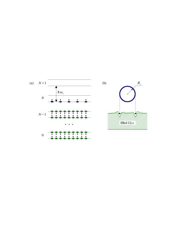
Figure 1: (a) Landau levels. Darkened ellipses symbolize electrons and arrows — their spins (b) A quasiparticle at the $N$th LL viewed as a ring-shaped object immersed into a medium formed by the filled lower LLs.

Technically, the high LL problem is equivalent to the more studied $N=0$ case if the bare Coulomb interaction $\tilde{v}_{0}(q)$ is replaced by the renormalized interaction

$$\tilde{v}(q)=\frac{\tilde{v}_{0}(q)}{\epsilon(q)}\left[L_{N}\left(\frac{q^{2}l^{2}}{2}\right)\right]^{2},$$ (2)

where $\epsilon(q)$ is the dielectric constant due to the screening by other LLs [13, 12] and the bracketed expression compensates for the difference in the form-factor

$$F_{N}(q)=L_{N}\left(\frac{q^{2}l^{2}}{2}\right)e^{-q^{2}l^{2}/4}$$ (3)

of the cyclotron orbit at $N$th and at the lowest LLs, with $L_{N}(z)$ being the Laguerre polynomial. In the next section we will discuss the consequences of having such an unusual interaction.

3 Charge density wave instability

The mean-field treatment of a partially filled LL amounts to the Hartree-Fock approximation, first examined in the present context by Fukuyama et al. It is worth pointing out the differences between their paper [14] and our own work [4] reviewed below in this section. The pioneering work of Fukuyama et al. [14] appeared in 1979. A few years later, after the discoveries of integral and fractional quantum Hall effects, it became clear that for the exception of dilute limit, the Hartree-Fock approximation is manifestly incorrect for the lowest LL case [15]. By 1995 when we started to work on the high LL problem, Ref. [14] has been effectively shelved away. In contrast to Ref. [14], who did not try to assess the validity of the Hartree-Fock approximation, our theory of a partially filled high LL [4] was based on this kind of approximation because it is the correct tool for the job. This point is elaborated further in Sec. 5. Another important difference from Ref. [14] is a parametric dependence of the wavevector $q_{*}$ of the CDW instability on the magnetic field: we find $q_{*}\propto B^{-1}$ instead of $\propto B^{-1/2}$ in the theory of Fukuyama et al. Finally, the physical picture of ring-shaped quasiparticles that guided our intuition is quite novel and applies only for high LLs.

Within the Hartree-Fock approximation, the free energy of the system is given by

$$F_{\rm HF}=\frac{1}{4\pi l^{2}}\sum_{q}\tilde{u}_{\rm HF}(q)|\langle\tilde{\Delta}(q)\rangle|^{2}+k_{B}T\sum_{X}\langle n_{X}\ln n_{X}+(1-n_{X})\ln(1-n_{X})\rangle,$$ (4)

where $\tilde{\Delta}(q)=(2\pi l^{2}/L_{x}L_{y})\sum_{X}e^{-iq_{x}X}a^{\dagger}_{X+q_{y}l^{2}/2}a_{X-q_{y}l^{2}/2}$ are guiding center density operators, $L_{x}$ and $L_{y}$ are system dimensions, $a^{\dagger}_{X}$ ($a_{X}$) are creation (annihilation) operators of Landau basis states $|X\rangle$, and $n_{X}=a^{\dagger}_{X}a_{X}$ are their occupation numbers subject to the constraint $\sum_{X}\langle n_{X}\rangle=L_{x}L_{y}\nu_{N}/(2\pi l^{2})$. Here and below we assume that $0<\nu_{N}<1$ because the states with $1<\nu_{N}<2$ are the particle-hole transforms of the states with $2-\nu_{N}$ and do not require a special consideration. The Hartree-Fock interaction potential is defined by $\tilde{u}_{\rm HF}(q)=(1-\delta_{q,0})\tilde{u}_{H}(q)-\tilde{u}_{F}(q)$, where

$$\tilde{u}_{H}(q)=\tilde{v}(q)e^{-q^{2}l^{2}/2},\quad\tilde{u}_{\rm ex}(q)=2\pi l^{2}u_{H}(ql^{2})$$ (5)

are its direct and exchange components (tildes denote Fourier transforms) [4]. Their $q$-dependence is illustrated in Fig. 2.

Figure 2: Direct, exchange, and the total Hartree-Fock potentials in $q$-space for $N=5$ and $r_{s}=0.5$. [Reproduced with permission from Fig. 2 of Ref. [4] (a)].

The inherent feature of $\tilde{u}_{HF}(q)$ is a global minimum at

$$q_{*}\approx 2.4/R_{c},$$ (6)

where it is negative, $\tilde{u}_{\rm HF}(q_{*})<0$. Within the Hartree-Fock theory, it leads to a charge density wave (CDW) formation at low enough temperatures $T$ [14]. Indeed, at high temperatures the entropic term dominates and the equilibrium state is a uniform uncorrelated liquid with $\langle n_{X}\rangle=\nu_{N}$ and $\langle\tilde{\Delta}(q)\rangle=\delta_{q,0}\nu_{N}$. At lower $T$, it is more advantageous to forfeit some entropy but gain some interaction energy by creating a guiding center density modulation $\langle\tilde{\Delta}_{q}\rangle\neq 0$ with wavevector $q=q_{*}$.

Since the quasiparticles are extended ring-shaped objects, the actual quasiparticle density modulation in any of our states is given by the product of the amplitude $\tilde{\Delta}(q)$ of the guiding center density wave and the cyclotron orbit form-factor:

$$\tilde{\rho}(q)=\tilde{\Delta}(q)F_{N}(q).$$ (7)

The physical electric charge modulation in the system is further suppressed by the additional factor of $\epsilon(q)$ due to the screening by the lower LLs. A peculiarity of the $N\gg 1$ case is that $q_{*}$ is very close to the first zero $q_{0}$ of $\tilde{u}_{H}(q)$, which it inherits from the form-factor $F_{N}(q)$.  On the one hand, this means that the physical electric charge modulation is always rather small — a few percent in realistic experimental conditions. On the other hand, it explains why this instability develops in the first place. Indeed, usually the direct electrostatic interaction is repulsive and dominates over a weak attraction due to exchange. In our system $\tilde{u}_{H}(q)$ vanishes at the “magic” wavevector $q_{0}$ because no charge density is induced, $\rho(q_{0})=0$. As a result, the exchange part dominates and gives rise to a range of $q$’s around $q_{0}$ where the net effective interaction $\tilde{u}_{\rm HF}(q)$ is attractive, which leads to the instability.

The nodes of $F_{N}(q)$ responsible for the vanishing of $\rho(q)$ exist for a purely geometric reason that the quasiparticle orbitals are extended objects of a specific ring-like shape. The size of the orbitals is uniquely defined by the total density and the total filling factor. These two facts make the position of the global minimum $q_{*}$ very insensitive to approximations contained in the Hartree-Fock approach as well as many microscopic details, e.g., the functional form of $\epsilon(q)$, thickness of the 2D layer, which affects $\tilde{v}_{0}(q)$, etc. At asymptotically large $N$ where the rings are very narrow, $F_{N}(q)$ is closely approximated by a Bessel function $J_{0}(qR_{c})$; hence, Eq. (6). Surprisingly, Eq. (6) is quite accurate even at $N\sim 1$.

The mean-field transition temperature $T_{c}^{\rm mf}$ can be estimated as the point where the stability criterion $1/\epsilon_{\rm tot}(q)<1$ of the uniform liquid state is first violated. Here $\epsilon_{\rm tot}(q)$ is the total dielectric function, including both the lower and the topmost LLs. A simple derivation [16] within the (time-dependent) Hartree-Fock approximation gives

$$\epsilon_{\rm tot}(q)=\epsilon(q)\left\{1+\tilde{u}_{H}(q)\left[\frac{2\pi l^{2}k_{B}T}{\nu_{N}(1-\nu_{N})}-\tilde{u}_{\rm ex}(q)\right]^{-1}\right\}.$$ (8)

The $T$-dependence of this function at $q=q_{*}$ is sketched in Fig. 3.

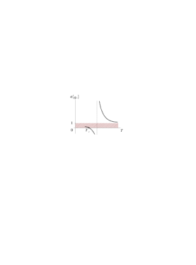
Figure 3: $T$-dependence of the dielectric function of the liquid state. The unstable region is hatched.

The stability criterion leads to the estimate

$$k_{B}T_{c}^{\rm mf}=\frac{\nu_{N}(1-\nu_{N})}{2\pi l^{2}}|\tilde{u}_{HF}(q_{*})|.$$ (9)

For $r_{s}\sim 1$, $N\gg 1$, and $\nu_{N}=1/2$, it can be approximated by

$$k_{B}T_{c}^{\rm mf}(\nu_{N}=1/2)\approx 0.02\hbar\omega_{c}.$$ (10)

Compared to the expression originally given in Ref. [4](b), a certain $1/N$ term is omitted here, out of precaution that the Hartree-Fock approximation, which is valid in the large-$N$ limit, may not have enough accuracy to describe $1/N$-corrections. This caveat should always be kept in mind when using numerical estimates of $k_{B}T_{c}^{\rm mf}$, such as those reported in Ref. [17]. For the typical experimental situation [6, 7], Eq. (9) gives $T_{c}^{\rm mf}\sim 1{\rm K}$.

4 Mean-field phase diagram

4.1 Charge density wave transition

A more systematic way to study the CDW transition is via a Landau expansion of the free energy $F$ in powers of the order parameters $\langle\tilde{\Delta}({\bf q})\rangle$ where ${\bf q}$ are restricted to the locus of the soft modes, $|{\bf q}|=q_{*}$:

$$F=\sum\limits_{n=2}^{\infty}a_{n}(T)\sum\limits_{{\bf q}_{1}+{\bf q}_{2}+\ldots+{\bf q}_{n}=0}\prod\limits_{i=1}^{n}\langle\tilde{\Delta}({\bf q}_{i})\rangle.$$ (11)

Note that in the quasiclassical large-$N$ limit, the order parameter $\langle\Delta({\bf r})\rangle$ is proportional to the local filling factor, $\langle\Delta({\bf r})\rangle=\nu_{N}({\bf r})/2\pi l^{2}$.

The above linear stability criterion is equivalent to the condition $a_{2}>0$. At $\nu_{N}=\frac{1}{2}$ where the cubic term vanishes by symmetry, $a_{3}=0$, the Landau theory’s estimate for $T_{c}$ coincides with Eq. (9). It predicts a second-order transition [14, 18], which occurs by a condensation of a single pair of harmonics, whose direction is chosen spontaneously, e.g., ${\bf q}=\pm q_{*}\hat{\bf x}$. The resultant low-temperature state is a unidirectional CDW or the stripe phase. Away from the half-filling, $a_{3}\neq 0$. Hence, at $\nu_{N}\neq\frac{1}{2}$ the transition is of the first order, takes place at a temperature somewhat higher than predicted by Eq. (9), and is from the uniform liquid into a CDW phase with the triangular lattice symmetry [14, 18], the bubble phase, see Fig. 4 (left).

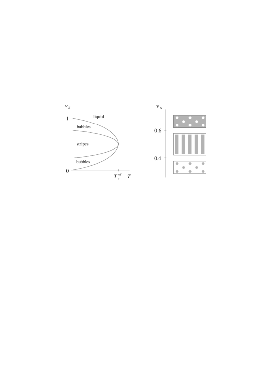
Figure 4: Left: Mean-field phase diagram. Right: Guiding center density domain patterns at $T=0$. Shaded and blank areas symbolize filled and empty regions, respectively.

Near its onset, the CDW order brings about only a small modulation of the local filling factor, so that the topmost LL remains partially filled everywhere. As $T$ decreases, the amplitude of the guiding center density modulation increases and eventually forces expulsion of regions with partial LL occupation. The system becomes divided into (i) depletion regions where $\langle\Delta({\bf r})\rangle=0$ and local filling fraction is equal to $2N$, and (ii) fully occupied areas where $\langle\Delta({\bf r})\rangle=(2\pi l^{2})^{-1}$ and local filling fraction is equal to $2N+1$ (however, see Ref. [4] for a discussion of truly small $r_{s}$). At these low temperatures the bona fide stripe and bubble domain shapes become evident, see Fig. 4 (right).

4.2 Stripe to bubble transition

Near $T_{c}$, the Landau theory [18] predicts the stripe-bubble transition to be of the first order. This seems to be the case at $T=0$ as well, at least at large $N$, where the this transition occurs at $\nu_{N}\approx 0.39$ [4], see Fig. 5a. In systems with only short-range interactions a density-driven first order transition is accompanied by a global phase separation. An example is the usual gas-liquid transition. The densities $n_{s}$ and $n_{b}$ of the two co-existing phases are determined by Maxwell’s tangent construction, Fig. 5b.

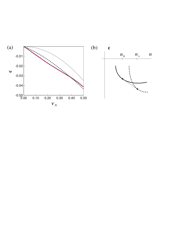
Figure 5: (a) The energy density $\epsilon$ in units of $\hbar\omega_{c}/2\pi l^{2}$ as a function of $\nu_{N}$ for the bubbles (thick solid line), the stripes (dashed line), and the uniform liquid (thin solid line) for $r_{s}=1$, $N\gg 1$, and $T=0$. (b) Schematics of the conventional tangent construction. As explained in the main text, it is too crude to account for the specifics of the long-range Coulomb interaction. For example, for the graph on the left, such a construction would give a vanishing $n_{b}$ and the maximum possible $n_{s}$, which is misleading.

In the present case the long-range Coulomb interaction changes the situation drastically. The macroscopic phase separation into two phases of different charge density is forbidden by an enormous Coulomb energy penalty. Only a phase separation on a finite lengthscale, i.e., domain formation may occur. Since stripes and bubbles are two the most common domain shapes in nature [20], it opens an intriguing possibility that bubble- or stripe-shaped domains of the stripe phase inside of the bubble phase may appear, i.e., the “superbubbles” (Fig. 6) or the “superstripes”. Their size would be determined by the competition between the Coulomb energy and the domain wall tension $\gamma$. The superbubbles would have a diameter

$$a\sim\frac{1}{n_{s}-n_{b}}\left(\frac{\gamma\kappa}{e^{2}}\right)^{1/2}$$ (12)

and increase the net energy density by $\sim\gamma p/a$, $p$ being the fraction of the minority phase. It turns out that this additional energy cost shrinks the range of the phase co-existence considerably compared to that in the conventional tangent construction. It may totally preclude the phase co-existence if

$$\frac{e^{2}\gamma}{\kappa}>(n_{s}-n_{b})^{2}\frac{d^{2}f_{s}}{dn^{2}}\frac{d^{2}f_{b}}{dn^{2}},$$ (13)

where $f_{s(b)}(n)$ is the free energy density of stripes (bubbles).

Incidentally, these considerations are also relevant for the main transition from the uniform state into the CDW one at $T=T_{c}$. We can think of the primary stripe and bubble phases as examples of a frustrated phase separation. At $\nu_{N}=1/2$ the conventional tangent construction would predict $k_{B}T_{c}=E_{\rm ex}/4$, whereas the actual (mean-field) transition temperature is lower [Eq. (10)] because of the extra energy density associated with the edges of the stripes.

Returning to the case of superbubbles, we estimate $d^{2}f_{s(b)}/dn^{2}\sim f_{s(b)}/n^{2}\sim E_{\rm ex}/n^{2}$ and $\gamma\sim E_{\rm ex}R_{c}n_{s}$ at $T=0$. The criterion (13) becomes $(n_{s}-n_{b})/n_{s}\lesssim R_{c}\sqrt{n_{s}}\sim\sqrt{N}$. Thus, we can be certain that the superstructures do not appear at high LLs. The cases of small $N$ or high temperatures require further study [16].

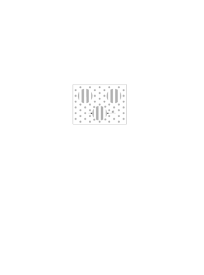
Figure 6: A cartoon of the conjectured superbubble phase.

4.3 Transitions caused by particle discreteness

With the periodicity of the bubble phase set by the preferred wavevector $q_{*}$, the area of unit cell of the bubble lattice is equal to $S_{0}=2\sqrt{3}\,\pi^{2}/q_{*}^{2}$. The number of particles per bubble is therefore $M=S_{0}\nu_{N}/2\pi l^{2}$. Using Eq. (6) we obtain [4]

$$M\approx 3\nu_{N}N,\quad N\gg 1.$$ (14)

It is natural to ask whether this formula should be taken literally, even when it predicts a nonintegral $M$. Strictly speaking, CDWs with a fractional number of particles per unit cell are not ruled out. However, we choose to ignore such an exotic possibility because early Hartree-Fock studies for the lowest Landau level [19] concluded that only the phases with integer-valued $M$ are stable. In our own numerical studies only integral $M$ were examined. The results are reproduced in Fig. 7 (see Ref. [5] for details). We found that the ground state value of $M$ never deviates from the prediction of Eq. (14) by more than unity at $N\leq 10$ and all $\nu_{N}$. This confirms the robustness of the optimal period $q_{*}$. It also suggests a practical rule for calculating the optimal $M$: one should evaluate the right-hand side of Eq. (14) and round it to the nearest integer.

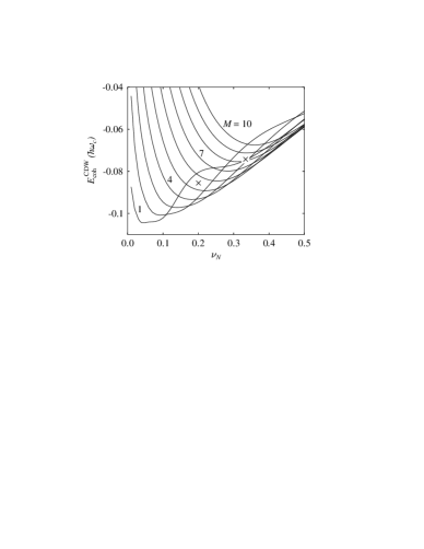
Figure 7: Cohesive energy $E_{\rm coh}^{\rm CDW}$ in a set of bubble phases with different number of particles per bubble $M$. $E_{\rm coh}^{\rm CDW}$ is defined as the interaction energy per particle $E_{\rm int}$ relative to the uncorrelated liquid [where $E_{\rm int}=-(\nu_{N}/2)E_{\rm ex}$]. Calculation parameters: $N=5$, $r_{s}=\sqrt{2}$, $T=0$. The crosses represent the Laughlin liquid energies. (Reproduced with permission from Fig. 2 of Ref. [5]).

Under the assumptions we made, $M$ exhibits a step-like behavior with unit jumps at a finite set of filling fractions. They correspond to the first-order transitions between distinct bubble phases. Everything said earlier about the possible phase co-existence near the first-order transitions applies here as well. For example, we do not expect any “bubbles of bubbles” at large $N$ although at moderate $N$ there is such a possibility. As $\nu_{N}$ decreases, the lattice constant of the bubble phase changes smoothly in between- and discontinuously at the transitions, but always remains close to $4\pi/\sqrt{3}\,q_{*}\approx 3.0R_{c}$. Only in the Wigner crystal state ($M=1$) the lattice constant is no longer tied to the cyclotron radius but is equal to $(4\pi/\sqrt{3}\,\nu_{N})^{1/2}l$, which is much larger than $R_{c}$ at $\nu_{N}\ll 1/N$.

One warning is in order here. While very useful, the Hartree-Fock approximation and the Landau theory of the phase transitions do not properly account for thermal and quantum fluctuations in 2D. A preliminary attempt to include these effects reveals additional phases and phase transitions of different order. The revised phase structure will be discussed in Sec. 7 below.

5 Validity of the Hartree-Fock theory

It has been mentioned above that the Hartree-Fock ground state of a partially filled LL is always a CDW. In particular, for $N=0$ it is a Wigner crystal [19]. It is well established by now that the latter prediction is in error at most filling fractions $\nu_{N}$. Instead, Laughlin liquids and other fractional quantum Hall states appear [15]. The Wigner crystal is realized only when $\nu_{N}$ is very small (dilute particles) or very close to $1$ (dilute holes). Below we present heuristic arguments and numerical calculations, which together make a convincing case that the situation at large $N$ is different, so that the ground state has a CDW order at all $\nu_{N}$ and not just in the dilute limit.

5.1 Quantum Lindenmann criterion

A heuristic criterion of the stability of periodic lattices is the smallness of the fluctuations about the lattice sites compared to the lattice constant. Unless $r_{s}$ is extremely small, the stripes and bubbles are contiguous completely filled (or completely depleted) regions of the topmost LL. In this situation the fluctuating objects are the edges of the stripes and bubbles. Using the suitably modified theory of the quantum Hall edge states (see Sec. 9), one can estimate their fluctuations $\delta r$ to be of the order of the magnetic length, $\delta r\sim l$. Since the period $\Lambda$ of the stripe and bubble lattices is at least a few $R_{c}=\sqrt{2N+1}\,l$, the Lindenmann criterion $\delta r\ll\Lambda$ is well satisfied, and so the CDW states should be stable at any $\nu_{N}$ and sufficiently large $N$. Basically, when the amplitude of the local filling factor modulation is appreciable and the stripes (bubbles) are so wide, they are very “heavy,” quasiclassical objects and quantum fluctuations are unable to induce a quantum melting of their long-range crystalline order. This is in contrast to the small $N$ case where the quantum fluctuations in the real space are of the order of the lattice constant except in the dilute limit.

5.2 Diagrammatic arguments

In a work [18] published soon after our original papers [4], Moessner and Chalker systematically analyzed the perturbation theory series for the partially filled high LL problem. They were able to achieve definitive results under two simplifying assumptions: (a) there is no translational symmetry breaking and (b) the range $R$ of the quasiparticle interaction is smaller than $l$. [This interaction is given by the inverse Fourier transform of $\tilde{v}_{0}(q)/\epsilon(q)$]. Under such conditions the Hartree-Fock diagrams were shown to dominate in the $N\gg 1$ limit. This is a very important result. Even though it enables us to make controlled statements only about the high-temperature uniform state, it certainly enhances the credibility of the Hartree-Fock results at all $T$. Due to the screening by the lower LLs embodied in the dielectric function $\epsilon(q)$ [Eq. (2)], the effective range $R$ of interaction turns out to be of the order of [12] $a_{B}=\hbar^{2}\kappa/me^{2}=l\sqrt{2/\nu r_{s}^{2}}$; thus, condition (b) is satisfied at $N\gg r_{s}^{-2}$, which is not too restrictive in practice.

There is still an interesting albeit academic question of what happens at truly small $r_{s}$ and intermediate filling factors where $1\ll N\ll r_{s}^{-2}$, so that $R\gg l$. It will be discussed shortly below.

5.3 CDW vs Laughlin liquids

Obvious competitors of the CDW states at simple odd-denominator fractions $\nu_{N}=1/(2k+1)$ are the Laughlin liquids. The interaction energy per particle in a Laughlin liquid can be found summing a rapidly converging series [21]

$$E_{\rm LL}=-\frac{\nu_{N}}{2}E_{\rm ex}+\frac{\nu_{N}}{\pi}\sum_{K=1}^{\infty}c_{K}V_{K},$$ (15)

where $V_{K}$ are Haldane’s pseudopotentials

$$V_{K}=\frac{1}{2\pi}\int\!d^{2}q\,\tilde{u}_{\rm H}(q)\,F_{K}(\sqrt{2}\,q),$$ (16)

$E_{\rm ex}$ (briefly introduced in Sec. 2 as a characteristic energy scale) is defined by

$$E_{\rm ex}=\tilde{u}_{\rm ex}(0)/(2\pi l^{2}),$$ (17)

and $c_{K}$ are coefficients calculable by the Monte-Carlo method [21, 5]. Numerically, about a dozen terms in the series (15) are needed to get an accurate value of $E_{\rm LL}$ at $\nu_{N}=\frac{1}{3}$ and $\nu_{N}=\frac{1}{5}$. In the large-$N$ limit we can also derive an analytical estimate, guided by the asymptotic relation

$$V_{K}\simeq\tilde{u}_{\rm ex}(2\sqrt{K}/l)/l^{2},\quad K\gg 1.$$ (18)

It indicates that $E_{\rm LL}$ is determined by the behavior of $\tilde{u}_{\rm ex}(q)$ at $q\sim l^{-1}$. Since the exchange and the direct interaction potentials are linked by the Fourier transform [cf. Eq. (5)], $\tilde{u}_{\rm ex}$ has the effective range of $R/l^{2}$ in the $q$-space [4]. Thus, two cases have to be distinguished.

1. $R\ll l$.— Physically, this corresponds to $N\gg\max\{1,r_{s}^{-2}\}$ (recall that the interaction range $R$ is of the order of $a_{B}$). Provided $R\ll l$, only first few terms in the series (15) are important, leading to the estimate $E_{\rm LL}\sim\tilde{u}_{\rm ex}(1/l)/l^{2}$. On the other hand, the interaction energy per particle in the CDW ground state, $E_{\rm CDW}\sim-\tilde{u}_{\rm ex}(q_{0})/l^{2}\sim-E_{\rm ex}$, is significantly lower, i.e., the CDW wins. In the practical case of $r_{s}\sim 1$, the CDW should be lower in energy than the Laughlin liquids at $N\geq N_{c}$ where $N_{c}$ is a small number. The numerical calculations reviewed below indicate that this “critical” number is $N_{c}=2$.

2. $R\gg l$.— This regime appears in the parameter window $1\ll N\ll r_{s}^{-2}$. It is mostly of academic interest because it can be realized only in very high density 2D systems where $r_{s}\ll 1$. Such systems are unavailable at present.

The theoretical analysis proceeds as follows. It turns out that Eq. (18) is correct with a relative accuracy $1/\ln N$ even for moderate $K$. With the same accuracy we can replace all $V_{K}$’s in Eq. (15) by $2\pi E_{\rm ex}$. Using the sum rule $\sum_{K}c_{K}=(1-\nu_{N}^{-1})/4$ [21], we arrive at the asymptotic formula

$$E_{\rm LL}\simeq-E_{\rm ex}/2,$$ (19)

which is of the same order as $E_{\rm CDW}$. To compare the energies of the two states, we have to exercise some care. Skipping the derivation, which relies heavily on another sum rule [19], for the Hartree-Fock states

$$\textstyle\sum|\langle\tilde{\Delta}({\bf q})\rangle|^{2}=\nu_{N},$$ (20)

we quote only the final result,

$$E_{\rm CDW}\simeq-E_{\rm ex}/2.$$ (21)

It signifies that the Laughlin liquid and the CDW have the same energy with a relative accuracy of $1/\ln N$. We may understand this surprising near equality as follows. Consider a system of particles interacting via a long-range two-body potential $v(r)$, which is nearly constant up to a distance $R$ and then gradually decays to zero at larger distances. The particles are presumed to be spread over a uniform substrate “of opposite charge” with which they interact via a potential $-n_{0}v(r)$. This fixes the average particle density to be $n_{0}$. It is easy to see that for any configuration of particles, which is uniform on the lenghscale of $R$, two potentials nearly cancel each other: (i) the total potential created at the location of a given particle by all the other particles of the system and (ii) the potential due to the substrate. The net potential is equal to $\Sigma=-v(0)$ because the particle does not interacts with itself. Due to the pairwise nature of the interaction, the interaction energy per particle (including the interaction with the substrate) is one half of $\Sigma$, i.e., $-v(0)/2$. Now we just need to recall from Sec. 2 that the energy of the self-interaction in our system is $E_{\rm ex}$ to recognize Eqs. (19) and (21) as particular cases of this general relation.

The above discussion has several implications. First, it clarifies the physics behind the arguments of Moessner and Chalker [18] that the CDW states are likely to face a strong competition from certain uniform states when the interaction is sufficiently long-range, $R\gg l$. Second, it leaves the nature of the ground state at $1\ll N\ll r_{s}^{-2}$ an open question at the moment. The CDW states seem to be favored in numerical calculations done for $2\leq N\leq 10$ and both $r_{s}\sim 1$ and $r_{s}\ll 1$ (see below). Truly high $N$ have not been investigated yet.

One intriguing possibility is the emergence of novel phases where the CDW ordering is not static but dynamic. One particular example is a quantum nematic phase, which can be visualized as a “soup” of fluctuating stripes. Such phases are actively discussed both in the context of the quantum Hall effect [22, 23, 24, 25, 26, 27] and the high-temperature superconductivity [28, 29, 30]. We would like to reiterate that an experimental search for these exotic phases would require very special samples, e.g., with $r_{s}$ much lower than presently available.

5.4 Numerical results

Trial wavefunctions.— The analytical estimates for $E_{\rm LL}$ and $E_{\rm CDW}$ derived above become accurate only at very large $N$. At moderate $N$ the comparison of trial states has to be done numerically. The procedure of calculating the energies of Laughlin liquids has been outlined above. It relies on the mapping of the $N$th LL problem onto a problem at the lowest LL with the modified interaction, Eq. (2). To compute the energy of a Hartree-Fock CDW state we use the same trick: the trial state is chosen from the Hilbert space of the lowest LL, but the interaction potential is appropriately modified.

The first step is to define the wavefunction of a single bubble:

$$\Psi_{0}\{{\bf r}_{k}\}=\prod\limits_{1\leq i<j\leq M}(z_{i}-z_{j})\times\exp\left(-\sum\limits_{i=1}^{M}\frac{|z_{i}|^{2}}{4l^{2}}\right),$$ (22)

where $z_{j}=x_{j}+iy_{j}$ are complex coordinates of $M$ quasiparticles that compose this bubble. A well-known property of the Vandermonde determinant indicates that $\Psi_{0}$ is in fact, a Hartree-Fock state. It is easy to see also that $\Psi_{0}$ defines the most compact arrangement of $M$ quasiparticles allowed at the lowest LL, i.e., a circular droplet of a completely filled LL centered at the point $x=y=0$.

The trial state we studied is composed of bubbles arranged in triangular lattice. It can be obtained by replicating the bubble (22) and translating its multiple copies to the appropriate lattice sites. This has to be followed by the antisymmetrization with respect to particle exchanges among different bubbles. The resulting wavefunction does not have a simple explicit form. Fortunately, to calculate the Hartree-Fock energy we do not need the wavefunction but only the particle density, see Eq. (4) and Ref. [19]. An excellent approximation for the latter is simply the sum of the densities of the individual bubbles. Strictly speaking, it is not a fully self-consistent solution of the nonlinear Hartree-Fock equations because of a small nonorthogonality among the wavefunctions of different bubbles. However, even the nearest bubbles are effectively so far away from each other that the deviations from the self-consistency are extremely small. If desired, the degree of self-consistency can be further improved using an iterative procedure of the relaxation type with the described density distribution as the initial guess. We have done this kind of calculations [5] and found that the iterations lower the energy of the state by less than one part in $10^{6}$, which does not affect the comparison with the Laughlin liquid energy (known much less accurately).

On the basis of such calculations, we concluded that the CDW becomes the ground state at $\nu_{N}=\frac{1}{3}$ for $N\geq 2$ and at $\nu_{N}=\frac{1}{5}$ for $N\geq 3$. For the latter fraction and $N=2$ the energies of the two trial states are so close that no definite conclusion could be made. Nevertheless, in practice the samples always contain some amount of disorder, which would favor the CDW state over the liquid state. Therefore, we established $N_{c}=2$ as the “critical” LL index where the transition from the Laughlin liquids to CDW phases occurs. $N_{c}$ turned out to be the same both for $r_{s}\sim 1$ and $r_{s}\ll 1$, and whether or not we included the effect of the finite-thickness of the 2D layer [5].

Since the fractional quantum Hall effect (FQHE) is traditionally associated with the Laughlin states while the CDW does not exhibit the FQHE, our results imply that the FQHE is restricted to the lowest and the first excited LLs, $N=0$ and $N=1$. It is in principle impossible to observe the FQHE at $N\geq 2$, and to date no one has. We are therefore led to propose the global phase diagram of the 2D electron systems shown in Fig. 8.

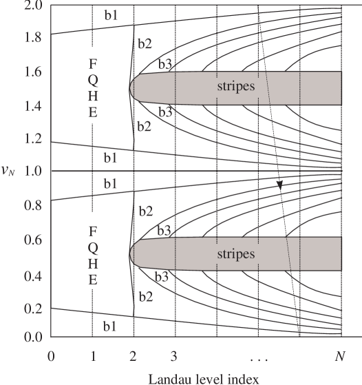
Figure 8: The global phase diagram of a 2D electron system in the axes $(N,\nu_{N})$ for the practical case $r_{s}\lesssim 1$ (schematically). The labels “b1”, “b2”, etc. denote the bubble phases with 1, 2, etc. particles per unit cell. As the magnetic field decreases, the system traces a zigzag path through this diagram, which starts at the lower left corner and proceeds along continuous segments $(N,0)\rightarrow(N,2)$ connected by discontinuous jumps $(N,2)\rightarrow(N+1,0)$. One such jump is shown by the dashed line with the arrow. In principle, points away from the zigzag path can also be sampled if the functional form of the bare interaction can be modified sufficiently strongly compared to the Coulomb law.

Exact diagonalization of small systems.— Strong evidence in favor of the CDW order in a partially filled $N\geq 2$ LL has been given by Rezayi, Haldane, and Yang [31], who studied systems up to 14 electrons by means of the direct numerical diagonalization of the Hamiltonian. Crucial for their success was employing periodical boundary conditions along the $\hat{\bf x}$ and $\hat{\bf y}$-directions (torus geometry). This setup avoids imposing the defects into the CDW lattice, aligns the CDW in a specific direction (which facilitates its detection), and enables to deduce the number of particles per unit cell simply from the multiplicity of the ground state manifold. Rezayi, Haldane, and Yang found no evidence of incompressible FQHE states at $2\leq N\leq 6$ and $\nu_{N}=\frac{1}{4},\frac{1}{3},\frac{2}{5}$, etc. Instead, they reported the ground state degeneracies and quasi-Bragg peaks in the structure factor fully consistent with the formation of the stripe phase near the half-filling and a bubble phase at $\frac{1}{3}$ and $\frac{1}{4}$. The periodicity deduced from the quasi-Bragg peak positions agreed with the Hartree-Fock prediction (6) within a few percent.

Density matrix renormalization group.— Shibata and Yoshioka [32] studied $N=2$ case using another powerful numerical technique, the density matrix renormalization group. Although not exact, it is presumed to be highly accurate both for the ground state energy and the ground state wavefunction. They were able to study larger systems, up to 18 electrons. Shibata and Yoshioka presented pair correlation functions unambiguously showing the stripe and bubble phases and pinpointed the transition point between them to be at $\nu_{N}\approx 0.38$.

6 Experimental evidence for stripes and bubbles

6.1 Resistance anisotropy

The existence of the stripe phase as a physical reality was evidenced by a conspicuous magnetoresistance anisotropy observed near half-integral fractions of high LLs [6, 7]. This anisotropy develops at low temperatures, $T\lesssim 0.1\,{\rm K}$, and only in very clean samples. The anisotropy is the largest at $\nu=9/2$ ($N=2$, $\nu_{N}=1/2$) and decreases with increasing LL index. At $T=25\,{\rm mK}$ it remains discernible up to $\nu\sim 11\frac{1}{2}$ whereupon it is washed out, presumably, due to residual disorder and/or finite temperature. The main anisotropy axes seem to be always oriented along the crystallographic axes of the GaAs crystal: $[1\bar{1}0]$ (the high-resistance direction) and $[110]$ (the low-resistance one). Especially striking are the data obtained using the square samples in the van-der-Pauw measurement geometry: at $\nu=9/2$ the resistances along the two principal directions differ by three orders of magnitude. However, one has to keep in mind that the van-der-Pauw measurements exaggerate the bare anisotropy of the resistivity tensor [33], due to current channeling along the easy (low-resistance) direction. Indeed, Hall-bar measurements, which provide a faithful representation of the resistivity tensor, show much smaller but still a very significant anisotropy up to 7:1. Once the current distribution effects are taken into account, the following picture emerges. At $T\gtrsim 0.1\,{\rm K}$, the transport is isotropic. As $T$ decreases, the resistivity along the $[110]$ direction ($\rho_{yy}$) decreases but only slightly. In contrast, the resistivity in the $[1\bar{1}0]$ direction ($\rho_{xx}$) rapidly increases, growing by almost an order of magnitude when $T$ drops down to $25\,{\rm mK}$. The anisotropy is the largest at $\nu_{N}=1/2$ but persists in a sizable interval $0.4<\nu_{N}<0.6$ of filling factors. Thus, as a function of $\nu_{N}$, $\rho_{xx}$ exhibits a peak resembling the quantum Hall transition peaks in dirtier samples at higher temperatures.

In contrast, the magnetotransport measurements near half-integral fillings of $N=0$ and $N=1$ LLs reveal no significant anisotropies and no peaks in the longitudinal resistance. Instead, the resistance exhibits a minimum as a function of $\nu_{N}$, which deepens at $T$ decreases [34]. Such unambiguous distinctions indicate that the electron ground states at high LLs $N\geq 2$ are qualitatively different from those in lower LLs. The $\nu=9/2$ is the fraction that demarcates the transition to the realm of novel high LL physics.

The emergence of the anisotropy is very natural once we assume that the stripe phase forms. It is based on two concepts: pinning of stripes by disorder and the edge-state transport. Each of these topics deserves a separate discussion, which will be given (in a brief form) in Secs. 10 and 9, respectively. Here we only sketch the basic ideas. The pinning serves the purpose of preventing the global sliding of the stripes. This singles out the edge-transport as the only viable mechanism of current propagation. The edges of the stripes can be visualized as metallic rivers, along which the transport is “easy.” The charge transfer among different edges, i.e., across the stripes, requires quantum tunneling and is “hard” because the stripes are effectively far away. Thus, if the stripes are preferentially oriented along the $[110]$ direction, the sample would exhibit the anisotropy of the kind observed in the experiment.

The physical mechanism responsible for the alignment of the stripes along the definite crystallographic direction is debated at present (see Sec. 12). In the absence of external aligning fields, the stripe orientation would be chosen spontaneously. On the other hand, due to enormous collective response of the stripe-ordered phase, the stripes can be easily oriented by a tiny bare anisotropy of the medium or the substrate.

6.2 New insulating states

The existence of the bubble phases at high LLs is supported by another striking experimental discovery: reentrant integral quantum Hall effect (IQHE) at $\nu\approx 4.25$ and $\nu\approx 4.75$. The Hall resistance at such filling factors is quantized at the value of the nearest IQHE plateau, while $\rho_{xx}$ and $\rho_{yy}$ show a deep minimum with an activated temperature dependence. The transport is isotropic in these novel insulating states, $\rho_{xx}\approx\rho_{yy}$. The current-voltage ($I$-$V$) characteristics exhibit pronounced nonlinearity, switching, and hysteresis. Such phenomena are hallmarks of the glassy behavior common for pinned crystalline lattices and conventional CDWs. Hence, these observations are fully consistent with the theoretical picture of a bubble lattice pinned by disorder. At $N=2$ we expect only two bubble phases: with two ($M=2$) and with one ($M=1$) particle per bubble. Both phases are subject to pinning and should be insulating at $T=0$. To understand the reentrancy phenomenon we have to take into account the finite-temperature effects. The $M=2$ bubble phase is more rigid than the $M=1$ (Wigner crystal) phase, and remains stable at temperatures where the Wigner crystal is already melted. As $\nu_{N}$ is varied towards the nearest integer, the insulating $M=2$ bubbles are replaced by a conducting plasma formed in place of the Wigner crystal. Close enough to the integer $\nu_{N}$, the plasma is so dilute that weakly interacting quasiparticles become localized by disorder and the conventional IQHE results.

Very recently, several more reentrant insulating states has been discovered also in the $N=1$ LL [35]. Their nature remains to be determined but it is tantalizing to suggest that these are also the bubbles phases.

6.3 Other experimental findings

It was shown in a set of remarkable experiments that the anisotropy near half-integral fillings can be strongly affected by an in-plane magnetic field $B_{\parallel}$. When applied along the easy resistance direction, the hard and the easy anisotropy axes interchange at $B_{\parallel}\gtrsim 0.5\,{\rm T}$ [36, 37]. When applied along the hard direction, the influence of $B_{\parallel}$ is much less pronounced and is to somewhat suppress the anisotropy. This intriguing behavior is thought to originate from the orbital effects of $B_{\parallel}$ in a finite-thickness 2D layer [17, 38]. They can be crudely described as squeezing of the cyclotron orbits in the direction perpendicular to $B_{\parallel}$. For such distorted orbits the stripe phase energy depends on the orientation of the stripes with respect to the in-plane magnetic field. Calculations based on a suitably generalized Hartree-Fock theory of the previous sections show that the preferred orientation of the stripes can be both parallel and perpendicular to the in-plane magnetic field, depending on microscopic details of the real systems [17, 38]. For the specific parameters believed to accurately describe the samples examined in Refs. [36, 37], the perpendicular orientation is preferred (in agreement with the experiment). However, further theoretical and experimental work is needed to fully understand these issues.

The magnetotransport anisotropy at high LLs was also observed for $p$-type GaAs samples [39].

The higher current transport regime near $\nu=9/2$ was investigated. Gradual increase in the differential resistance along the hard direction was reported. Compared to the strong nonlinearities at the reentrant IQHE states, it is a relatively weak effect.

Finally, the degree of anisotropy and the effect of the in-plane fields were found to be more pronounced in the lower spin subtend of the same Landau level. A possible explanation within the Hartree-Fock theory was recently suggested by Wexler and Dorsey [40].

7 Many faces of the stripe phase

In the wake of the experiments, a considerable amount of work has been devoted to the stripe phase in recent years [24, 43, 44, 45, 46, 47, 48, 49]. It led to the understanding that the “stripes” may appear in several distinct forms: an anisotropic crystal, a smectic, a nematic, and an isotropic liquid (Fig. 9). These phases succeed each other in the order listed as the magnitude of either quantum or thermal fluctuations increases. Thus, at small $N$ ($N=2,3$) or close to $T_{c}$ the phase diagrams of Fig. 4a and Fig. 8 need modifications to incorporate some (if not all) of those phases. The general structure of the revised phase diagram for the quantum ($T=0$) case was discussed in the important paper of Fradkin and Kivelson [24]. Pinpointing the new phase boundaries in terms of the conventional parameters $r_{s}$ and $\nu$ will require further analytical and numerical work. Once again, we wish to emphasize that at large $N$ these additional phases have very narrow regions of existence, if any. Let us now give the definitions of these intriguing phases and discuss their basic properties.

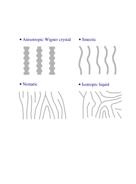
Figure 9: Sketches of possible stripe phases.

Stripe crystal.— This state may in principle be understood at the Hartree-Fock level. It was shown [44] that the initially proposed Hartree-Fock solution with smooth edges and a strictly 1D periodicity [4] is not the global energy minimum. A further gain in energy is attained once the stripes acquire a periodic modulation in the longitudinal direction, in antiphase on each pair of neighboring stripes. The resultant phase breaks the translational symmetry in both spatial directions and thus is equivalent to a 2D crystal. The unit cell of such a crystal is very anisotropic, with the aspect ratio of the order of $N:1$. However, there is only a single particle per unit cell; thus, this state is an anisotropic Wigner crystal. It is presumably the true ground state of the system at sufficiently large $N$ where the Hartree-Fock is deemed to be exact.

Smectic state.— The usual definition of the smectic is a “liquid with the 1D periodicity.” A smectic is less ordered than a crystal because the translational symmetry is broken only in one spatial direction. The rotational symmetry is of course broken as well. The smectic stripe phase can be thought of as a descendant of the stripe crystal where the longitudinal modulations on neighboring stripes persist locally, but have no long-range antiphase order because of dynamic phase slips. In other words, the neighboring stripes are unlocked [44]. In the thermodynamic limit this kind of state is equivalent to a stripe phase with no modulations (smooth edges), akin to the original Hartree-Fock solution [4]. The necessary condition for the smectic order is the continuity of the stripes. If the stripes are allowed to rupture, the dislocations are created. They destroy the 1D positional order and convert the smectic into the nematic.

Nematic state.— By definition, the nematic is an anisotropic liquid. There is no long-range positional order. As for the orientational order, it is long-range at $T=0$ and quasi-long-range (power-law correlations) at finite $T$. The nematic is riddled with dynamic dislocations. Other types of topological defects, the disclinations, may also be present but remain bound in pairs, much like vortices in the 2D $X$-$Y$ model.

Isotropic liquid.— Once the disclinations in the nematic unbind, all the spatial symmetries are restored. The resultant state is an isotropic liquid with short-range stripe correlations. As the fluctuations due to temperature or quantum mechanics increase further, it gradually crosses over to the “uncorrelated liquid” where even the local stripe order is obliterated.

8 Effective theories of the stripe phase

As often the case, the low-frequency long-wavelength physics of the system is governed by an effective theory involving a relatively small number of dynamical variables. The basic form of the effective theory is essentially fixed by the symmetry considerations. Let us outline how such theories are constructed for the various stripe states introduced in the previous section.

8.1 Stripe crystal

The low-energy dynamical variables of this state are the elastic deformation ${\bf u}=\{u_{x}({\bf r},t),u_{y}({\bf r},t)\}$ of the crystalline lattice and the effective description is basically the elasticity theory. In addition, we have to account for the long-range Coulomb interaction between the density fluctuations $n({\bf r},t)=-n_{0}\nabla{\bf u}$, where $n_{0}=\nu_{N}/(2\pi l^{2})$ is the average particle density at the $N$th LL. The symmetry arguments identify four nonvanishing elastic moduli: $c_{11}$, $c_{12}$, $c_{22}$, and $c_{44}$, so that the effective Hamiltonian takes the form

$$H = \frac{c_{11}}{2}(\partial_{x}u_{x})^{2}+\frac{c_{22}}{2}(\partial_{y}u_{y})^{2}+c_{12}\partial_{x}u_{y}\partial_{y}u_{x}+\frac{c_{44}}{8}(\partial_{x}u_{y}+\partial_{y}u_{x})^{2}$$ (23)

$$+ \frac{1}{2}n_{0}^{2}(\nabla{\bf u})u_{\rm H}(\nabla{\bf u}),$$

where $u_{\rm H}$ should be understood as the integral operator. The dynamics of the system is governed by the Lorentz force and can be studied with the help of the effective Lagrangean

$${\cal L}=mn_{0}\omega_{c}u_{y}\partial_{t}u_{x}-H.$$ (24)

Solving the corresponding equations of motion, we find the following excitation spectrum of lattice vibrations (magnetophonons):

$$\omega({\bf q})=\frac{\omega_{p}(q)}{\omega_{c}}q\left[\frac{c_{44}+(c_{11}+c_{22}-2c_{12}-c_{44})\sin^{2}2\theta}{4mn_{0}}\right]^{1/2}.$$ (25)

Here $\omega_{p}(q)=[n_{0}\tilde{u}_{\rm H}(q)q^{2}/m]^{1/2}$ is the plasma frequency and $\theta=\arctan(q_{y}/q_{x})$ is the angle between the propagation direction and the $\hat{\bf x}$-axis. For Coulomb interactions $\omega_{p}(q)\propto\sqrt{q}$ leading to the well-known dispersion relation [50] $\omega(q)\propto q^{3/2}$. In a strongly anisotropic stripe crystal, $c_{12},c_{44}\ll c_{11}$ causing the angular dependence $\omega({\bf q})\propto\sin 2\theta$ starting from relatively small $q$. All these results are valid for an idealized clean system. In reality the low-$q$ magnetophonon modes will be profoundly affected by disorder, which will be discussed in Sec. 10.

8.2 Smectic state

As mentioned above, the smectic state is most closely related to the original Hartree-Fock solution [4]. It may be visualized as Hartree-Fock stripes slightly decorrelated by phonon-like thermal fluctuations.

Harmonic approximation.— In the smectic only $u_{x}$ retains its direct meaning of the elastic displacement. On the other hand, the density fluctuations $n$ become an independent degree of freedom. For example, in the case of incompressible stripes, $n$ comes from the stripe width fluctuations, which are separate from the “shape” fluctuations described by $u_{x}$. The number of dynamical variables in the smectic and in the crystal is therefore the same. Moreover, the smectic can be thought of as a crystal that lost its shear rigidity because of phase slips between nearby crystalline rows. This intuitive picture enables us to deduce the effective theory for the smectic from Eqs. (23) and (24) by a certain reduction. Of course, at the end we should verify that we did not miss any terms allowed by symmetry. The first step is to formally reintroduce $u_{y}$ as a solution of the equation $\partial_{y}u_{y}=-n/n_{0}-\partial_{x}u_{x}$ and use it to replace all instances of $\partial_{y}u_{y}$ in Eq. (23). To ensure that the stripes are free to slide with respect to each other in the $\hat{\bf y}$-direction, the terms that depend on $\partial_{x}u_{y}$ should be dropped: $c_{12}\rightarrow 0$, $c_{44}\rightarrow 0$. Yet we need to be careful and recall that the complete elasticity theory always contains higher gradients such as $(\partial_{y}^{2}u_{x})^{2}$ [suppressed in Eq. (23)]. Once the coefficient in front of the first-order gradient term $(\partial_{y}u_{x})^{2}$ vanishes, higher gradients become dominant and must be included. The resultant effective Hamiltonian and the Lagrangean take the form

$$H=\frac{Y}{2}(\partial_{x}u)^{2}+\frac{K}{2}(\partial_{y}^{2}u)^{2}+\frac{1}{2}n(u_{\rm H}+\chi^{-1})n+Cn\partial_{x}u,$$ (26)

$${\cal L}=p\partial_{t}u-H,\quad\partial_{y}p=-m\omega_{c}(n+n_{0}\partial_{x}u).$$ (27)

Here we switched to notations more natural for the smectic: $u_{x}$ became $u$, $u_{y}$ was traded for the canonical momentum $p$, the sum $c_{11}+c_{22}$ became $Y$, etc. The physical meaning of new phenomenological coefficients is as follows. $Y$ and $K$ are the compression and the bending elastic moduli, $\chi$ is the compressibility, and $C=2\pi l^{2}Yd\ln\Lambda/d\nu_{N}$ accounts for the dependence of the mean interstripe separation $\Lambda$ on the average filling factor.

Since the number of dynamical variables in the smectic is the same as in the crystal state, the collective mode count is also unchanged. We will keep referring to them as magnetophonons. Solving the equations of motion for $n$ and $u$ we obtain the dispersion relation of such magnetophonons [45]:

$$\omega({\bf q})=\frac{\omega_{p}(q)}{\omega_{c}}\frac{q_{y}}{q}\left[\frac{Yq_{x}^{2}+Kq_{y}^{4}}{mn_{0}}\right]^{1/2}.$$ (28)

Unless propagate nearly parallel to the stripes, $\omega({\bf q})$ is proportional to $\sin 2\theta\,q^{3/2}$. Unlike in the stripe crystal, this relation is obeyed even at $q\rightarrow 0$ (again, in the absence of disorder or orienting fields). One immediate consequence of this dispersion is that the largest velocity of propagation for the magnetophonons with a given $q$ is achieved when $\theta=45^{\circ}$.

Thermal fluctuations and anharmonisms.— From Eq. (26) we can readily calculate the mean-square fluctuations of the stripe positions at finite $T$, e.g.,

$$\langle[u(0,0)-u(0,y)]^{2}\rangle=2\int\frac{d^{2}q}{(2\pi)^{2}}\frac{k_{B}T}{Yq_{x}^{2}+Kq_{y}^{4}}(1-e^{ik_{y}y})=\frac{k_{B}T}{2\sqrt{YK}}|y|.$$ (29)

This formula is valid if $y$ is large so that magnetophonons with wavevectors $q_{y}\lesssim 1/y$ can be treated classically [$\hbar\omega({\bf q})\ll k_{B}T$]. As one can see, at any finite temperature magnetophonon fluctuations are growing without a bound; hence, the positional order of a 2D smectic is totally destroyed [51] at sufficiently large distances along the $\hat{\bf y}$-direction, $|y|\gg\Lambda\sqrt{YK}/k_{B}T\equiv\xi_{y}$. Similarly, along the $\hat{\bf x}$-direction, the positional order is lost at lengthscales larger than $\xi_{x}=(Y/K)^{1/2}\xi_{y}^{2}$.

Another type of excitations, which decorrelate the stripe positions are the aforementioned dislocations. The dislocations in a 2D smectic have a finite energy $E_{D}\sim K$. At $k_{B}T\ll E_{D}$ the density of thermally excited dislocations is of the order of $\exp(-E_{D}/k_{B}T)$ and the average distance between dislocations is $\xi_{D}\sim\Lambda\exp(2k_{B}T/E_{D})$. At low temperatures $\xi_{x},\xi_{y}\ll\xi_{D}$; therefore, the following interesting situation emerges (Fig. 10). On the lengthscales smaller than $\xi_{y}$ (or $\xi_{x}$, whichever appropriate) the system behaves like a usual smectic where Eqs. (26–28) apply. On the lengthscales exceeding $\xi_{D}$ it behaves like a nematic [52]. In between the system is a smectic but with very unusual properties. It is topologically ordered (no dislocations) but possesses enormous fluctuations. In these circumstances the harmonic elastic theory becomes inadequate and anharmonic terms must be included. The most important anharmonisms are captured in the following elastic Hamiltonian, which should be substituted in place of the first two terms in Eq. (26) [51]:

$$H_{el}=\frac{Y}{2}\Bigl{[}\partial_{x}u-\frac{1}{2}(\nabla u)^{2}\Bigr{]}^{2}+\frac{K}{2}(\partial_{y}^{2}u)^{2}.$$ (30)

It can be easily checked that the expression inside the square brackets, which is the compressional strain, is invariant under rotations of the reference frame by an arbitrary angle $\phi$. For example, if in the initial reference frame $u=0$, then in the new frame $u(x,y)=(1-\cos\phi)x+\sin\phi\,y$ so that $\partial_{x}u-\frac{1}{2}(\nabla u)^{2}=0$.

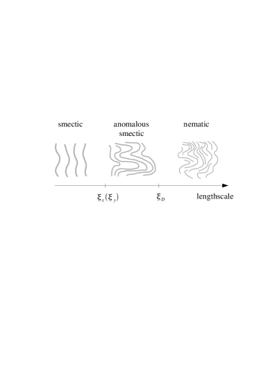
Figure 10: Portraits of the stripe phase on different lengthscales.

What is the role of anharmonisms? As shown by Golubović and Wang [53], they cause power-law dependence of the parameters of the effective theory on the wavevector ${\bf q}$:

$$Y\sim Y_{0}(\xi_{y}q_{y})^{1/2},\quad K\sim K_{0}(\xi_{y}q_{y})^{-1/2},$$ (31)

for $q_{x}\ll\xi_{x}^{-1}(q_{y}\xi_{y})^{3/2}$, $q_{y}\ll\xi_{y}^{-1}$, and

$$Y\sim Y_{0}(\xi_{x}q_{x})^{1/3},\quad K\sim K_{0}(\xi_{x}q_{x})^{-1/3},$$ (32)

for $q_{x}\ll\xi_{x}^{-1}$ and $q_{y}\ll\xi_{y}^{-1}(q_{x}\xi_{x})^{2/3}$. The lengthscale dependence of the parameters of the effective theory is a common feature of fluctuation-dominated phenomena. Other famous examples include the criticality near phase transitions and in systems at their lower critical dimension, such as the 2D $X$-$Y$ model. It should be mentioned that the lower critical dimension for the smectic order is $d=3$ [51], so that the 2D smectic is below its lower critical dimension. This is the reason why the scaling behavior (31) and (32) does not persist indefinitely but eventually breaks down above the lengthscale $\xi_{D}$ where the crossover to the thermodynamic limit of the nematic behavior commences.

Equations (31) and (32) indicate that the compression modulus decreases while the bending modulus increases as the lengthscale grows. This can be understood from the following qualitative reasoning. Thermal fluctuations create a lot of wiggles on the stripes. When an external compressional stress is applied, it can be relieved not just by compression but by flattening of the stripes. Since the latter involves unbending of the crumpled stripes and the bending costs less energy than the compression ($q^{4}$ instead of $q^{2}$), the apparent compressional modulus $Y$ is smaller than its bare value $Y_{0}$. Similarly, when one attempts to bend crumpled stripes, some compression is necessarily involved, and so the bending modulus $K$ appears larger.

The scaling shows up not only in the static properties such as $Y$ and $K$ but also in the dynamics. The role of anharmonisms in the dynamics of conventional 3D smectics has been investigated by Mazenko et al. [54] and also by Kats and Lebedev [55]. For the quantum Hall stripes the analysis had to be done anew because here the dynamics is totally different. It is dominated by the Lorentz force rather than a viscous relaxation in the conventional smectics. This task was accomplished in Ref. [45]. The calculation was based on the Martin-Siggia-Rose formalism combined with the $\epsilon$-expansion below $d=3$ dimensions. One set of results concerns the spectrum of the magnetophonon modes, which becomes

$$\omega({\bf q})\sim\sin\theta\cos^{7/6}\theta\,(\xi_{x}q)^{5/3}\frac{\omega_{p}(\xi_{x}^{-1})}{\omega_{c}\xi_{x}}\sqrt{\frac{Y_{0}}{mn_{0}}}.$$ (33)

Compared to the predictions of the harmonic theory, Eq. (28), the $q^{3/2}$-dispersion changes to $q^{5/3}$. Also, the maximum propagation velocity is achieved for the angle $\theta\approx 53^{\circ}$ instead of $\theta=45^{\circ}$. These modifications, which take place at long wavelengths, are mainly due to the renormalization of $Y$ in the static limit and can be obtained by combining Eqs. (28) and (32). Less obvious dynamical effects peculiar to the quantum Hall smectics include a novel dynamical scaling of $Y$ and $K$ as a function of frequency and a specific $q$-dependence of the magnetophonon damping [45].

The latter issue touches on an important point. Our effective theory defined by Eqs. (26) and (27) is based on the assumption that $u$ and $n$ are the only low-energy degrees of freedom. It is probably well justified at $T\rightarrow 0$ but becomes incorrect at higher temperatures. The point of view taken in Ref. [45] is that in the latter case thermally excited quasiparticles (“normal fluid”) should appear and that they should bring dissipation into the dynamics of the magnetophonons.

Another intriguing possibility is for quasiparticles or other additional low-energy degrees of freedom to exist even at $T=0$. Such more complicated smectic states are not ruled out and are interesting subjects for future study.

8.3 Nematic state

Much like loosing the shear rigidity due to phase slips converts a crystal to a smectic, loosing the compressional rigidity due to mobile dislocations can convert a 2D smectic into a nematic. The collective degree of freedom associated with the nematic ordering is the angle $\phi({\bf r},t)$ between the local normal to the stripes ${\bf N}$ and the $\hat{\bf x}$-axis orientation. Due to inversion symmetry, ${\bf N}$ and $-{\bf N}$, i.e., $\phi$ and $\phi+\pi$ are equivalent, that is why ${\bf N}$ is often referred to as the director rather than a vector [51]. The effective Hamiltonian for ${\bf N}$ is dictated by symmetry to be

$$H_{N}=\frac{K_{1}}{2}(\nabla{\bf N})^{2}+\frac{K_{3}}{2}|\nabla\times{\bf N}|^{2}.$$ (34)

The coefficients $K_{1}$ and $K_{3}$ are termed the splay and the bend Frank constants [51]. They control the cost of the two possible elementary types of director nonuniformity shown in Fig. 11. Note that in the smectic phase $\phi=-\partial_{y}u$. This entails the relation $K_{3}\simeq K$ between the parameters of the nematic and its parent smectic. On the other hand, the value of $K_{1}$ is expected to be determined largely by the properties of the dislocations [52]. The elastic part has a particularly simple form if $K_{1}=K_{3}$, in which case $H_{N}=(K_{3}/2)(\nabla\phi)^{2}$ just like in the $X$-$Y$ model.

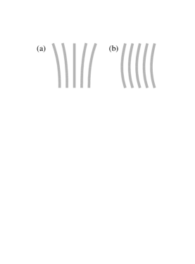
Figure 11: Splay (a) and bend (b) distortions in a nematic.

Another obvious degree of freedom in the nematic are the density fluctuations $n({\bf r},t)$. A peculiar fact is that in the static limit $n$ is totally decoupled from ${\bf N}$, and so it does not enter Eq. (34). However, since the nematic is less ordered than even a smectic, the question about extra low-energy degrees of freedom or additional quasiparticles become especially relevant. We believe that different types of quantum Hall nematics are possible in nature. In the simplest case scenario ${\bf N}$ and $n$ are the only low-energy degrees of freedom. This type of state has been studied by Balents [23] and recently by the present author [25]. It was essentially postulated that the effective Largangean takes the form

$${\cal L}=\frac{1}{2}\gamma^{-1}(\partial_{t}{\bf N})^{2}-H.$$ (35)

(As hinted above, the full expression contains also couplings between $\partial_{t}{\bf N}$ and mass currents but they become vanishingly small in the long-wavelength limit). The collective excitations are charge-neutral fluctuations of the director. They have a linear dispersion,

$$\omega({\bf q})=q\sqrt{{K_{1}}{\gamma}\cos^{2}\theta+{K_{3}}{\gamma}\sin^{2}\theta},$$ (36)

and resemble spinwaves in the $X$-$Y$ quantum rotor model.

Also discussed in Ref. [25] was a dislocation-mediated mechanism of the smectic-nematic transition within the framework of duality transformations developed earlier by Toner and Nelson [52], Toner [56], and Fisher and Lee [57]. This theory predicts the existence of a second excitation branch with a small gap. This gapped mode can be considered a descendant of the magnetophonon mode of the parent smectic.

Very recently, Radzihovsky and Dorsey [27] formulated a different theory of the quantum Hall nematics, whose predictions disagree with our Eqs. (35) and (36). Logically, there are two possibilities. Either, as mentioned above, there are several distinct kinds of nematic states possible in nature or some of the theoretical constructions advanced in Refs. [23, 25, 27] are incorrect. To resolve these issues it is imperative to bring the discussion from the level of effective theory to the level of quantitative calculations. One promising direction is to investigate concrete trial wavefunctions of quantum nematics, e.g., the one proposed by Musaelian and Joynt [22]:

$$\Psi=\prod\limits_{j<k}(z_{j}-z_{k})[(z_{j}-z_{k})^{2}-a^{2}]\times\exp\Bigl{(}-\sum_{j}|z_{j}|^{2}/4l^{2}\Bigr{)}.$$ (37)

Here $a$ is a complex parameter that determines the degree of orientational order and the direction of the stripes. This particular wavefunction corresponds to $\nu=\frac{1}{3}$. (As explained earlier, it can also be used investigate the higher Landau level states with $\nu_{N}=\frac{1}{3}$). Recently, the work in this direction was continued by Ciftja and Wexler [26].

Other contributions to the theory of quantum Hall nematics have been focused on a finite temperature case. They include a work of Fradkin et al [41] who investigated the role of external anisotropy field in the 2D $X$-$Y$ formulation and also a paper by Wexler and Dorsey [40], where a quantitative Hartree-Fock analysis of the Toner-Nelson disclination unbinding scenario has been done.

It is worth mentioning that in the quantum case the chain of transitions crystal $\rightarrow$ smectic $\rightarrow$ nematic $\rightarrow$ isotropic liquid may or may not be realized in full. A finite-size study by Rezayi et al. [58] suggests that the transition from the smectic to an isotropic phase, as the interaction parameters are varied away from their $N=2$ Coulomb values, can also occur via a first-order transition, without the intermediate nematic phase. The resultant isotropic state is highly correlated and has little in common with the “uncorrelated” Hartree-Fock liquid. The natural candidates for the isotropic state include a Fermi-liquid-like state of composite fermions and a Pfaffian (Moore-Read) state [58]. Understanding all these competing quantum orders and transitions between them remains a major intellectual challenge. In contrast, the phase structure at larger $N$, away from the “transition point” $N=2$, is much simpler and is adequately captured by the Hartree-Fock theory.

9 Edge state models

Another theoretical approach to the physics of the stripe phases is based on the edge-state formalism. The advantages of the edge-state models are two-fold. First, they allow to bridge the gap between the microscopic theory and the formulations based on the elasticity theory or hydrodynamics (albeit under some crucial simplifying assumptions). Second, they enable one to calculate not only collective but also single-particle properties, such as the tunneling density of states. On the other hand, being more specialized than the hydrodynamics, the edge models have a somewhat restricted domain of validity. The models considered so far [24, 43, 48, 49] apply when the stripes are incompressible. i.e., when they are contiguous regions of $\nu_{N}=1$ separated by sharp boundaries from the regions with $\nu_{N}=0$. In our opinion the edge state models are better suited for describing the crystal and the smectic states. In the nematic state stripes exhibit violent quantum (or thermal) fluctuations and the picture of well defined sharp edges is questionable.

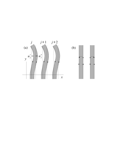
Figure 12: (a) Geometrical meaning of variables in the edge-state effective theory. (b) Backscattering.

The first step in constructing the edge theory is to identify the low-energy degrees of freedom with the deviations $u^{j}_{\pm}$ of the stripe boundaries from their equilibrium positions $x^{j}_{\pm}=(j\pm\nu_{N}/2)\Lambda$, see Fig. 12a. Such deviations induce extra 1D guiding center densities along the edges, $\rho^{j}_{\pm}=\pm u^{j}_{\pm}/(2\pi l^{2})$. The next step is to find an effective Hamiltonian $H$ that governs the interaction among $\rho^{j}_{\pm}$. To this end it is convenient to introduce the Fourier transform

$$\tilde{\rho}_{\sigma}({\bf q})=\Lambda\sum_{j}\exp(-iq_{y}x^{j}_{\sigma})\int dye^{-iq_{y}y}\rho_{\sigma}^{j}(y),$$ (38)

and define the center-of-mass stripe displacement $u_{x}$ and the net local density fluctuation per unit area,

$$\tilde{u}_{x}({\bf q})=2\pi l^{2}\left[\exp(\frac{i}{2}q_{x}\nu_{N}\Lambda)\tilde{\rho}_{+}({\bf q})+\exp(-\frac{i}{2}q_{x}\nu_{N}\Lambda)\tilde{\rho}_{-}({\bf q})\right],$$ (39)

$$\tilde{n}({\bf q})=\Lambda^{-1}\left[\exp(\frac{i}{2}q_{x}\nu_{N}\Lambda)\tilde{\rho}_{+}({\bf q})-\exp(-\frac{i}{2}q_{x}\nu_{N}\Lambda)\tilde{\rho}_{-}({\bf q})\right].$$ (40)

The general symmetry requirements compel the long-wavelength part $H_{0}$ of the Hamiltonian to take the form (26), reproduced here for convenience:

$$H_{0}=\frac{Y}{2}(\partial_{x}u_{x})^{2}+\frac{K}{2}(\partial_{y}^{2}u_{x})^{2}+\frac{1}{2}n(u_{\rm H}+\chi^{-1})n+Cn\partial_{x}u_{x}.$$ (41)

The edge-state formalism enables one go further and obtain quantitative estimates for the phenomenological parameters $Y$, $K$, $\chi$, and $C$ from the microscopic Hamiltonian. It should be clarified that the exact calculation of these parameters remains out of reach for the moment. Available derivations [43, 44, 47, 40, 49] are certainly not exact. It can be shown [16] that all of them rely on one specific approximation scheme, the time-dependent Hartree-Fock approximation (TDHFA). In the spirit of the discussion in the previous sections, we expect the TDHFA to be quantitatively accurate at $N\gg 1$ but only qualitatively correct in the case of current experimental interest, $N\sim 2$. Let us therefore proceed with the exposition of the field-theoretic edge-state formalism.

Besides $H_{0}$, the full effective Hamiltonian contains another term $H_{2q_{F}}$, whose importance was first emphasized by Fradkin and Kivelson [24]. To clarify its origin let us recall that in the Landau gauge $A=(0,Bx,0)$ each single-particle basis state $|X\rangle$ has a definite momentum in the $\hat{\bf y}$-direction, proportional to the mean value $X$ of the $x$-coordinate in such a state, $k_{y}=X/l^{2}$. In the simplest mean-field realization of the stripes, a given state is filled if $k_{y}\in(x^{j}_{+}/l^{2},x^{j}_{-}/l^{2})$ and is empty otherwise. Thus, $k_{y}=x^{j}_{\pm}$ play the role of Fermi points in an equivalent quasi-1D electron system. Note that “$+$” (“$-$”) stands for the sign of the Fermi velocity near a given Fermi points, in the positive (negative) $\hat{\bf y}$-direction. The density fluctuations $\rho^{j}_{\pm}$ propagate along the edges only in the direction specified by this sign. Such a property is called chirality. Thus, the stripe phase is characterized by a Manhattan grid of alternating chiral edge states. From this perspective, $H_{0}$ describes the particle-particle interactions, which cause only small changes in $X$ and thus small momentum transfer in the vicinity of the Fermi points. Another low-energy process is to scatter particles between different Fermi points, e.g., $x^{j}_{+}/l^{2}\rightarrow x^{j}_{-}/l^{2}$ and $x^{j+1}_{-}/l^{2}\rightarrow x^{j+1}_{+}/l^{2}$, see Fig. 12b. Such scattering acts must involve a pair of particles to conserve the total momentum: one particle gains and the other looses the same amount of momentum, $2q_{F}^{e}\equiv(x^{j}_{+}-x^{j}_{-})/l^{2}=\nu_{N}\Lambda/l^{2}$. $H_{2q_{F}}$ accounts precisely for the processes of this type. Since they cause the reversal of the propagation direction for the particles involved, it is natural to call it backscattering. Remarkably, it is possible [42] to express $H_{2q_{F}}$ in terms of density fluctuations $\rho^{j}_{\pm}$. Without going into details, we quote the final result [24, 43],

$$H_{2q_{F}} = -\sum_{j}\lambda^{e}\cos[(\phi^{j}_{+}-\phi^{j}_{-})+(\phi^{j+1}_{-}-\phi^{j+1}_{+})]$$ (42)

$$- \sum_{j}\lambda^{h}\cos[(\phi^{j}_{-}-\phi^{j-1}_{+})+(\phi^{j}_{+}-\phi^{j+1}_{-})]$$

Here $\phi^{j}_{\pm}$ are auxiliary dynamical variables related to $\rho^{j}_{\pm}$ as follows:

$$\rho^{j}_{\pm}=\partial_{y}\phi^{j}_{\pm}/(2\pi).$$ (43)

The phenomenological parameters $\lambda^{a}$ are proportional to $\tilde{u}_{\rm H}(2q_{F}^{a})$ but in general depends on how the theory is formulated (the ultraviolet cutoff). In principle, interactions can scatter the particles not only between nearest edges but also next-nearest ones, etc. The corresponding amplitudes are proportional to $\tilde{u}_{\rm H}(q)$ where $q$ is the appropriate momentum transfer. Since $\tilde{u}_{\rm H}$ decreases exponentially at such large $q$, these other processes are expected to have negligible effect. Thus, the total Hamiltonian is $H=H_{0}+H_{2q_{F}}$.

The final step in constructing the effective edge theory is determining the kinetic term. Either from Wen’s bosonization theory [42] of by comparing Eqs. (27) and (43), one can come to the conclusion that $\phi^{j}_{\pm}$ and $\rho^{j}_{\pm}$ are canonically conjugate variables, so that the appropriate Lagrangean is

$${\cal L}=\frac{\hbar}{4\pi}\sum_{j,\sigma=\pm}\sigma\partial_{t}\phi^{j}_{\sigma}\partial_{y}\phi^{j}_{\sigma}-H_{0}-H_{2q_{F}}.$$ (44)

Let us now explain how this theory can lead either to crystalline or to smectic behavior. The idea is to treat $H_{2q_{F}}$ as a small perturbation [24, 43, 44, 47]. If this perturbation is irrelevant, in the long-wavelength low-frequency limit $H$ reduces to $H_{0}$ and ${\cal L}$ to the smectic form (27). On the other hand, if $H_{2q_{F}}$ is relevant, then the “$+$” and “$-$” edges of each stripe become strongly mixed so that a static $2q_{F}$ density modulation in the $\hat{\bf y}$-direction appears. Its spatial period is $a=2\pi/(2q_{F})=2\pi l^{2}/\nu_{N}\Lambda$; hence, the number of particles on a given stripe within one modulation period is $\nu_{N}\Lambda\times a/(2\pi l^{2})=1$. This can be visualized as a 1D chain of particles. The neighboring chains are locked in antiphase to lower their interaction energy. This state is an anisotropic Wigner crystal with the aspect ratio of the unit cell $\Lambda:a=(\nu_{N}/2\pi)(\Lambda/l)^{2}\sim N:1$. Two types of stripe crystals are possible. If the first term in $H_{2q_{F}}$ is relevant, it is an “electron” crystal, if the second term is relevant, it is a “hole” crystal.

The elasticity theory (23) of, e.g., the electron crystal can be recovered as follows. Since the first sum in Eq. (42) is relevant, the large fluctuations of the argument of the corresponding cosines are inhibited. It is legitimate to expand these cosines to arrive at

$$H_{2q_{F}}\rightarrow-\sum_{j}\frac{\lambda_{*}}{2}(u^{j}_{y}-u^{j+1}_{y}-\Lambda\partial_{y}u_{x})^{2},$$ (45)

$$u_{y}({\bf q})\equiv\frac{l^{2}}{\nu_{N}\Lambda}[\phi_{+}({\bf q})e^{i\Lambda q_{x}/2}-\phi_{-}({\bf q})e^{-i\Lambda q_{x}/2}].$$ (46)

In the long-wavelength limit it gives a term proportional to $(\partial_{x}u_{y}+\partial_{y}u_{x})^{2}$, which makes the shear modulus $c_{44}$ finite [cf. Eq. (23)]. A more careful treatment presumably recovers the remaining elastic constant $c_{12}$. Our choice of $u_{y}$ in Eq. (46) is not arbitrary because we want to preserve the physical interpretation of $u_{y}$ as the elastic displacement. This requires $H_{2q_{F}}$ to be invariant under the shift by a lattice constant, $u_{y}\rightarrow u_{y}+a$. Since $H_{2q_{F}}$ is invariant under the shift $\phi^{j}_{\pm}\rightarrow\phi^{j}_{\pm}+2\pi$, it fixes the coefficient of proportionality in Eq. (46) to the value given.

The relevance or irrelevance of $H_{2q_{F}}$ depends on the stiffness of the stripes measured, roughly, by the dimensionless parameter $Yl^{4}/\tilde{u}_{\rm H}(\pi/\Lambda)$. If it is small enough, then high-$q$ and $\omega$ fluctuations of $\phi^{j}_{\pm}$ and $u^{j}_{y}$ (either quantum or thermal) are sufficiently strong to cause effective averaging out of the cosines in $H_{2q_{F}}$. As a result, the coefficient $\lambda$ renormalizes to zero in the low $q$ and $\omega$ limit. In contrast, for rigid stripes, the averaging of the cosine terms is not important. The perturbative renormalization group (RG) analysis [43, 44, 47, 49] allows to make this argument more precise.  However, to decide between the crystal or the smectic behavior, the RG requires accurate estimates for $Y$ and other parameters of the edge theory as an input. Attempts to extract such parameters from the TDHFA for the case of current experimental interest, $N\sim 2$, led to contradictory statements in the literature [43, 47, 49]. In this regard, we wish to reiterate that at $N\sim 2$ the stripe phase is very fragile and faces a strong competition from other quantum Hall states. Therefore, the Hartree-Fock and its time-dependent extensions are not quantitatively reliable. At the present stage the controlled theoretical analysis can be envisioned only for large $N$, building on the work of Moessner and Chalker [18]. Note that the ratio $Yl^{4}/\tilde{u}_{\rm H}(\pi/\Lambda)$ becomes an $N$-independent number of the order of unity at $N\gg 1$ and $r_{s}\sim 1$.

Concluding this section, let us discuss the tunneling into the stripe phase from the normal metal. Two setups can be imagined: tunneling from a bulk metal or from an STM tip. In the first case the electron-electron interactions are screened by the metal, in the second they remain long-range. The differential tunneling conductance $G_{T}=dI/dV$ at bias voltage $V$ is proportional to the tunneling density of states $g(eV)$, which is defined by $g(E)=(1/\pi)\Im{\rm m}\tilde{G}_{R}(E/\hbar)$, $\tilde{G}_{R}(\omega)$ being the single-electron Green’s function,

$$G_{R}(t)=-i\theta(t)\langle\Psi(0)\Psi^{\dagger}(t)\rangle.$$ (47)

Here $\Psi^{\dagger}$ and $\Psi$ are the electron creation and annihilation operators. The crude overall behavior of $g(E)$ can be obtained at the Hartree-Fock level. In the simplest case of the smectic (unmodulated stripes), $g(E)$ is determined by the slope of the self-consistent potential $E(X)$ that defines the energies of the quasiparticle states $|X\rangle$,

$$g_{\rm HF}(E)=|4\pi l^{2}\Lambda(dE/dX)|^{-1}.$$ (48)

The tunneling density of states calculated according to this formula is nonvanishing in a finite interval of width $\sim E_{\rm ex}$ around $E=0$. At both ends of such an interval one finds two divergencies (van Hove peaks). The interior of the interval can be described as a shallow pseudogap, see Fig. 13. The negative-$E$ peak corresponds to tunneling into the states with $X$’s in the middle of the filled stripes and the positive-$E$ one — into the middle of the empty stripes. Conversely, at low energies (low $V$) the tunneling can only occur into points in a vicinity of stripe edges [4]. The Hartree-Fock results for $g(E)$ are certainly not exact. However, the van Hove peaks and the pseudogap are expected to be true features and the Hartree-Fock estimate for the energy separation between the peaks should be quite reliable. The largest deviations from the Hartree-Fock predictions should occur at low $E$, which we now address. We will use the evolution in the imaginary time $\tau=it$ picture common in quantum tunneling problems.

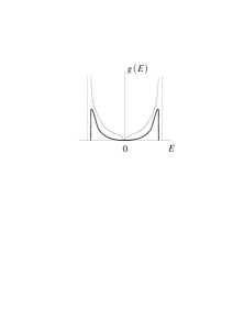
Figure 13: The sketch of the true tunneling density of states (solid line) and its Hartree-Fock approximation (dashed line).

Since the edges are effectively far away from one another, the incoming electron is initially accommodated into the closest edge, say, $j_{+}$. It produces a compact charge disturbance with a high Coulomb energy. The charge has to gradually spread over the entire area. This takes place by the emission of the magnetophonons. (In the context of the edge-state theories they are traditionally called edge magnetoplasmons). What is missing in the Hartree-Fock picture is precisely this relaxation from a point-like disturbance into an uniform state with an added quasiparticle of the given small energy $E$. Its net result is a suppression of the true $g(E)$ compared to $g_{\rm HF}(E)$. To calculate the suppression factor, one can use the bosonization prescription $\Psi\propto\exp(i\phi^{j}_{+})$ [42], which entails

$$\tilde{G}_{R}(i\omega_{n})\propto\int\limits_{0}^{\infty}d\tau\exp\Bigl{[}i\omega_{n}\tau-\frac{1}{2}\langle\phi^{j}_{+}(0)\phi^{j}_{+}(\tau)-\phi^{j}_{+}(0)\phi^{j}_{+}(0)\rangle\Bigr{]}.$$ (49)

This expression can be evaluated with the help of the effective action (44) and then analytically continued to real frequencies $i\omega_{n}\rightarrow\omega+i0$ [10]. For the smectic, such a calculation has been performed by Lopatnikova et al. [49]. They obtained $I(V)\propto\exp(-\sqrt{V_{0}/V})$ and $I(V)\propto\exp[-\ln^{2}(V_{0}/V)]$ for the Coulomb and short-range interaction case, respectively. The last formula was also obtained by Barci et al. [48]. As one can see, the tunneling conductance vanishes at zero voltage, which is a typical result for tunneling into a correlated electron system. For the crystal, the calculation is more difficult because the action is essentially nonlinear [the harmonic approximation (45) is not adequate for the tunneling problem]. It has not been reported in the literature. On the physical grounds, we expect the tunneling conductance to be exactly zero unless $eV$ exceeds the energy needed to nucleate a phase slip $u_{y}\rightarrow u_{y}+a$ (an analog of an interstitial in conventional crystals).

10 Pinning of stripes by disorder

Disorder in the form of randomly positioned impurities is expected to strongly affect the degree of the positional, orientational, and topological orders in the stripe phase at low $T$. According to modern understanding, none of these survives in the thermodynamic limit in two dimensions. However, in the most interesting case of weak disorder, the details of how each type of order is destroyed are subtly different. Let us start the discussion with the case of a smectic. Here the positional order is limited primarily by random elastic distortions. They can be characterized by the roughness function

$$f(r)=\langle[u({\bf r}^{\prime})-u({\bf r}^{\prime}+{\bf r})]^{2}\rangle,$$ (50)

so that the positional correlation length $\xi_{P}$ can be defined by the condition $f(\xi_{P})=\Lambda^{2}$. On the other hand, the correlation lengths for the topological order $\xi_{T}$ and orientational order $\xi_{O}$ are set by the mean distance between the disorder-generated dislocations and disclinations, respectively. Note that an appreciable magnetotransport anisotropy can be detected only if the sample size is smaller than $\xi_{O}$. This explains why samples of macroscopic dimensions $L\sim 0.25\,{\rm mm}$ show no anisotropy unless they are extremely pure [6, 7]. In addition to weakness of disorder, the gigantic $\xi_{O}$ in these experiments may have originated from a small bare anisotropy, which favored the alignment of the stripes along the $[110]$ direction. Indeed, an external anisotropy qualitatively modifies the smectic state properties by generating a finite tilt modulus $Y_{\perp}$. Correspondingly, the elastic part $H_{el}$ of the Hamiltonian becomes

$$H_{el}=\frac{Y}{2}\Bigl{[}\partial_{x}u+\frac{1}{2}(\nabla u)^{2}\Bigr{]}^{2}+\frac{Y_{\perp}}{2}(\partial_{y}u)^{2}+\frac{K}{2}(\partial_{y}^{2}u)^{2}.$$ (51)

The full Hamiltonian $H=H_{el}+H_{pin}$ also includes the interaction with disorder. It can be approximated by $H_{pin}=\int\exp[iq_{*}u({\bf r})]V({\bf r})$ where $V({\bf r})$ is a random short-range potential. The behavior of the static correlation functions, such as $f(r)$, as functions of $r$ and disorder strength has been evaluated within this model by Scheidl and von Oppen [59] building on the theory developed earlier for other pinned systems [60, 61]. Scheidl and von Oppen suggested that in the current experiments the characteristic lengthscales satisfy the chain of inequalities $\xi_{P}<\xi_{T}<L<\xi_{O}$, so that the stripe phase resembles an instantaneous snapshot of a nematic with no long-range positional order and a number of frozen-in dislocations.

Besides decorrellating the stripe positions, another interesting disorder effect in the smectic phase can be inducing quenched random $2q_{F}$-modulations along the stripes, as suggested by Yi et al. [47]. This is similar to the effect of impurities on a 1D “Wigner crystal” [62] (where without impurities the density is uniform because of strong quantum fluctuation). To properly describe this effect and its consequences, a comprehensive quantum theory of pinned smectics is required.

The pinning effects in the stripe crystal phase are qualitatively similar because $H_{el}$ is already not too different from the elastic Hamiltonian of an anisotropic crystal. The main difference is the doubling of the number of components of the elastic displacement field ${\bf u}=\{u_{x},u_{y}\}$.

The combined effects of finite temperature and disorder have not been investigated in any detail, but based on the extensive work done in other contexts [63, 64] we may expect a thermal depinning at a certain “glass transition temperature.”

Exceedingly interesting topic is the dynamics of pinned electron (liquid) crystals in high magnetic field. First of all, there are number of open questions in the general theory of pinned manifolds (such as CDWs, vortex lattices, magnetic domains, etc.). The current interests in this subject area include dislocation dynamics and non-equilibrium states (e.g., high electric field sliding phases). In addition to that, there are interesting dynamical effects unique to quantum Hall systems. For instance, in the recent years it was experimentally discovered [65] that even the linear response of a pinned Wigner crystal in a magnetic field is dramatically different from conventional expectations [66]. Typically, one anticipates the response to be dominated by low-frequency magnetophonon modes, which in the presence of pinning become localized wavepackets. Since the disorder is different in different parts of the sample, a considerable inhomogeneous broadening is expected. Instead, a sharp resonance-like mode in the microwave absorption spectrum appears (typically around $1\,{\rm GHz}$). Assuming that the quasiclassical description is adequate, Huse and the present author [67] explained the appearance of a narrow mode as a combined effect of the special Lorentz-force dynamics and long-range Coulomb interaction. However, the theory was done for the $T=0$ while the experimental line width seem to be dominated by thermal broadening. In fact, the thermal broadening is much more pronounced than one would naively expect and may reflect some nontrivial physics overlooked in a formulation based on harmonic elasticity theory [67]. The similar pinning resonance should exist in a stripe crystal as well and may even persists in a smectic phase. Since at high LLs all the energy scales are smaller, the pinning mode should have a lower frequency, perhaps, of the order of 100 MHz at $\nu=9/2$ for the kind of samples used in Refs. [6, 7].

11 Magnetotransport in the stripe phase

The magnetotransport in a partially filled Landau level is a problem of two extremes. In a perfectly clean system, it is completely trivial and amounts to the uniform sliding motion of all the particles in the direction perpendicular to the applied electric field, leading to $\sigma_{xx}=0$, $\sigma_{xy}=(e^{2}/h)\nu$. On the other hand, in the presence of disorder, the magnetotransport immediately becomes very complicated. Especially for the stripe phase, the magnetotransport theory is very incomplete at the moment. For instance, the transport in the nematic phase is a total enigma. Certain progress has been achieved regarding the crystal and the smectic phases. As discussed above, pinning by random impurities eliminates the possibility of a global sliding motion of the electron liquid under the action of an external electric field. As a result, the stripe crystal is an insulator. In the smectic, gapless edge states may exist in which case the edge transport is possible. The quasiparticles travel along the edges in the direction prescribed by the edge chiralities and also be scattered between the edges by impurities. The scattering probability depends on the distance between the edges. For a general filling fraction $\nu_{N}$ the widths of the filled (electron) and empty (hole) stripes are unequal, and so the corresponding mean-free paths are also different, $l_{e}\neq l_{h}$. On a large scale the quasiparticle motion resembles a random walk with unequal elementary steps: along the stripes, it is a properly weighted average of $l_{e}$ and $l_{h}$, across the stripes it is the interstripe separation $\Lambda$. If we assume that (a) the stripes are continuous and are all oriented along the $\hat{\bf y}$-direction, (b) the scattering occurs only between nearest edges, and (c) quantum localization effects can be neglected, then a simple calculation leads to the following formulas for the components of the conductivity tensor [43, 68]:

$$\sigma_{xx}=\frac{e^{2}}{h}\frac{\Lambda^{-1}}{l_{e}^{-1}+l_{h}^{-1}},\quad\sigma_{yy}=\frac{e^{2}}{h}\frac{\Lambda}{l_{e}+l_{h}},\quad\sigma_{xy}=\frac{e^{2}}{h}\Bigl{(}N+\frac{l_{e}}{l_{e}+l_{h}}\Bigr{)}.$$ (52)

At the symmetric point $l_{e}=l_{h}$, the transport anisotropy ratios are given by $R=\sigma_{yy}/\sigma_{xx}=\rho_{xx}/\rho_{yy}=l_{e}^{2}/\Lambda^{2}$, which is large for dilute impurities. However, there are reasons to doubt that Eq. (52) directly applies to the experimental practice. Indeed, from the empirical estimate $R\sim 7$ one would conclude that $l_{e}\sim 2.6\Lambda\sim 0.2\,\mu{\rm m}$, which seems too short for the extreme purity samples used. The most probable reason for reduction of the anisotropy ratio compared to the idealized formula (52), is the absence of high degree of the orientational and topological orders. As explained above, the pinning by disorder introduces pronounced elastic deformations as well as dislocations and disclinations into the perfect stripe pattern. Thus, in a more realistic model the above condition (a) should be abandoned. This leads to a view of the low-temperature stripe phase is a collection of elongated puddles of $\nu_{N}=1$ state preferentially aligned in a certain direction (a kind of frozen nematic). The conductivity tensor can no longer be calculated in any simple way; however, it satisfies the generalized Dykhne-Ruzin semicircle law [69]

$$\sigma_{xx}\sigma_{yy}+(\sigma_{xy}-\sigma_{0})^{2}=(e^{2}/2h)^{2},\quad\sigma_{0}\equiv(e^{2}/2h)(2N+1),$$ (53)

pointed out by von Oppen, Halperin, and Stern [68]. In addition, exactly at half-filling $\sigma_{xy}=\sigma_{0}$ and the product rule [69, 43, 9] applies:

$$\sigma_{xx}\sigma_{yy}=(e^{2}/2h)^{2}.$$ (54)

Both relations agree quite well with the low-temperature experimental data at $\nu=9/2$ [8], which is encouraging. However, one has to be careful with drawing conclusions from such a comparison. The status of Eqs. (53) and (54) in the quantum domain is poorly understood and is even somewhat compromised by the lack of agreement with the data from dirtier samples. The situation is complicated by a unconventional behavior of the resistivity peak at $\nu=9/2$ (low-$T$ width saturation), precisely where the product rule is supposed to apply.

At higher temperatures where the CDW amplitude is small, the stripe edges are not well defined objects. It is better to describe the system as a “compressible liquid.” A new type of transport theory is needed in this regime. It is reasonable to assume, for example, that the stripes can be depinned already by a vanishingly small electric field, so that a global sliding of the electron liquid becomes possible. If disorder is sufficiently smooth, it would be similar to a flow of a viscous 2D liquid across a disordered substrate [16].

Sufficiently close to $T_{c}$ the dislocations must become highly mobile so that the stripe phase should behave as a nematic on all relevant lenghtscales. A phenomenological approach to the magnetotransport in this regime was advocated by Fradkin et al. [41]. They argue on the basis of symmetry that the deviation of the resistivity ratio $R=\rho_{xx}/\rho_{yy}$ from unity is proportional to the degree of the orientational order in the nematic. Under a simplifying assumption that the Frank constants are equal, they map the problem onto a 2D $X$-$Y$ model in the presence of a small orienting field. Using the Monte-Carlo results for the latter model, they fitted the experimental data for $R$ with the help of two free parameters.

12 Other topics

The space constraints force us to switch to a telegraphic-style overview of the remaining topics explored in connection with the CDW phases in high LLs.

One of those is the bare anisotropy that aligns the stripes in the $[110]$ direction. Its origin remains unclear. A careful study by Cooper et al. [71] has ruled out a few earlier suggestions that included substrate morphology [70], vicinal steps from a slight miscut of the wafer, and a small anisotropy of the effective mass [72, 73]. One of the remaining viable alternatives is piezoelectric effects [74]. The orienting effects of the in-plane magnetic field was further studied in wide quantum wells [78]. The combination of the empirical findings and the Hartree-Fock calculations suggest that the anisotropy is indeed tiny, $\sim 1\,{\rm mK}$ per electron. The corresponding analysis for the $p$-type GaAs [39] has also been performed [75]. It is more involved because of the band-structure anisotropy. The preferred stripe orientation was predicted to sensitively depend on various details such as the width of the quantum well.

The time-dependent Hartree-Fock calculations of the collective modes of the stripe crystal has been done by Fertig et al. [46, 47]. At low $q$’s the results are in agreement with the general structure predicted by the effective theories, Secs. 7 and 9. At higher $q$ a new feature is revealed: a roton-like minimum at $q\approx q_{*}$, which may be thought of as a precursor to the stripe-bubble transition.

Stripe phases in bilayer systems have been studied by Brey and Fertig [76] and also by Demler et al. [77]. The additional layer degree of freedom leads to a rich phase diagram. Some of that physics may be operational in wide quantum wells [78].

The emergence of the CDW indicates some sort of instability of the conventional uniform FQHE states at high LLs. Such an instability was indeed found in numerical studies of Scarola et al. [79] who relied on the composite-fermion theory. It was also discussed within the phenomenological mean-field composite-boson formulation [73].

13 Conclusions

The physics of high LLs has fledged into a fast growing and vibrant field. Despite a significant progress, a multitude of open problems remains. Some of them are brand new (the existence of qualitatively novel states of matter such as quantum nematic), others are venerable quantum Hall problems with a new twist (the integral quantum Hall transition in the stripe phase). The real progress in understanding these intriguing yet difficult problems is likely to be tied with future experimental advances. It should be mentioned that the magnetotransport studies have certainly not exhausted their potential. Ongoing fantastic achievements in sample fabrication continue to deliver the ever more perfect systems, which should expedite the discovery of new phases. A fresh example is the aforementioned group of new insulating states in the $N=1$ LL of $3.1\times 10^{7}\,{\rm cm}^{2}/{\rm Vs}$ mobility sample [35] (Sec. 6). Besides relying on increasing sample quality, it may be interesting to experiment with different sizes of already available samples in search for the sequence of “spaghetti” phases sketched in Fig. 10. On the other hand, finite-frequency tools, such as microwaves, surface acoustic waves, and inelastic light scattering will provide other invaluable information inaccessible by the dc magnetotransport. Finally, the real-space imaging [80, 81] of the stripes and bubbles would be the most definitive proof of their existence.

It is a safe bet that we will see a great number of surprises and new developments in this area.

14 Acknowledgements

This work is supported by the MIT Pappalardo Fellowships Program in Physics. I would like to thank A. A. Koulakov, B. I. Shklovskii, and V. M. Vinokur for previous collaboration during which the key ideas and insights surveyed in these notes have emerged. I also wish to thank B. I. Shklovskii for valuable comments on the manuscript.

References

- [1] P. T. Coleridge, P. Zawadzki, and A. Sachrajda, Phys. Rev. B 49, 10 798 (1994).
- [2] L. P. Rokhinson and V. J. Goldman, unpublished; S. A. J. Wiegers, M. Specht, L. P. Lévy, M. Y. Simmons, D. A. Ritchie, A. Cavanna, B. Etienne, G. Martinez, and P. Wyder, Phys. Rev. Lett. 79, 3238 (1997); for a discussion, see M. M. Fogler and B. I. Shklovskii, Phys. Rev. B 52, 17 366 (1995).
- [3] N. Turner, J. T. Nicholls, E. H. Linfield, K. M. Brown, G. A. C. Jones, and D. A. Ritchie, Phys. Rev. B 54, 10 614 (1996).
- [4] (a) A. A. Koulakov, M. M. Fogler, and B. I. Shklovskii, Phys. Rev. Lett. 76, 499 (1996); (b) M. M. Fogler, A. A. Koulakov, and B. I. Shklovskii, Phys. Rev. B 54, 1853 (1996).
- [5] M. M. Fogler and A. A. Koulakov, Phys. Rev. B 55, 9326 (1997).
- [6] M. P. Lilly, K. B. Cooper, J. P. Eisenstein, L. N. Pfeiffer, and K. W. West, Phys. Rev. Lett. 82, 394 (1999).
- [7] R. R. Du, D. C. Tsui, H. L. Störmer, L. N. Pfeiffer, and K. W. West, Solid State Commun. 109, 389 (1999).
- [8] J. P. Eisenstein, M. P. Lilly, K. B. Cooper, L. N. Pfeiffer, and K. W. West, Physica E 9, 1 (2001); J. P. Eisenstein, Solid State Commun. 117, 132 (2001).
- [9] F. von Oppen, B. I. Halperin, and A. Stern, Advances in Quantum Many-Body Theory, vol. 3, ed. by R. F. Bishop, N. R. Walet, and Y. Xian (World Scientific, 2000) (also available as cond-mat/0002087).
- [10] G. D. Mahan, Many-Particle Physics (Plenum, New York, 1990).
- [11] At least for thin 2D layers, see X.-G. Wu and S. L. Sondhi, Phys. Rev. B 51, 14 725 (1995); N. R. Cooper, Phys. Rev. B 55, 1934 (1997).
- [12] I. L. Aleiner and L. I. Glazman, Phys. Rev. B 52, 11 296 (1995).
- [13] I. V. Kukushkin, S. V. Meshkov, and V. B. Timofeev, Usp. Fiz. Nauk 155, 219 (1988) [Sov. Phys. Usp. 31, 511 (1988)].
- [14] H. Fukuyama, P. M. Platzman, and P. W. Anderson, Phys. Rev. B 19, 5211 (1979).
- [15] For review, see Quantum Hall Effect edited by R. E. Prange and S. M. Girvin (Springer-Verlag, New York, 1990); C. Glattli, Chapter I in this book; R. Shankar, Chapter II ibid.
- [16] M. M. Fogler, unpublished.
- [17] T. Stanescu, I. Martin, and P. Philips, Phys. Rev. Lett. 84, 1288 (2000).
- [18] R. Moessner and J. T. Chalker, Phys. Rev. B 54, 5006 (1996).
- [19] D. Yoshioka and H. Fukuyama, J. Phys. Soc. Jpn. 47, 394 (1979); D. Yoshioka and P. A. Lee, Phys. Rev. B 27, 4986 (1983).
- [20] M. Seul and D. Andelman, Science, 267, 476 (1995).
- [21] S. M. Girvin, Phys. Rev. B 30, 558 (1984); S. M. Girvin, A. H. MacDonald, and P. M. Platzman, Phys. Rev. B 33, 2481 (1986).
- [22] K. Musaelian and R. Joynt, J. Phys. Cond. Mat. 8, L105 (1996).
- [23] L. Balents, Europhys. Lett. 33, 291 (1996).
- [24] E. Fradkin and S. A. Kivelson, Phys. Rev. B 59, 8065 (1999).
- [25] M. M. Fogler, cond-mat/0107306.
- [26] O. Ciftja and C. Wexler, cond-mat/0108119.
- [27] L. Radzihovsky and A. T. Dorsey, cond-mat/0110083.
- [28] J. M. Tranquada et. al., Phys. Rev. Lett. 73, 1003 (1994); J. M. Tranquada et. al., Nature 375, 561 (1995); S. Mori, C. H. Chen, and S.-W. Cheong, Nature 392, 473 (1998).
- [29] V. J. Emery, E. Fradkin, and S. A. Kivelson, Nature 393, 550 (1998).
- [30] J. Zaanen, O. Y. Osman, H. V. Kruis, Z. Nussinov, and J. Tworzydlo, cond-mat/0102103 and references therein.
- [31] E. H. Rezayi, F. D. M. Haldane, and K. Yang, Phys. Rev. Lett. 83, 1219 (1999); ibid 85, 5396 (2000).
- [32] N. Shibata and D. Yoshioka, Phys. Rev. Lett. 86, 5755 (2001).
- [33] S. H. Simon, Phys. Rev. Lett. 83, 4223 (1999).
- [34] At ultralow temperatures the fraction exhibits a quantum Hall effect: a deep minimum in with the activated behavior and a concomitant quantum Hall plateau in , see W. Pan, J.-S. Xia, V. Shvarts, D. E. Adams, H. L. Stormer, D. C. Tsui, L. N. Pfeiffer, K. W. Baldwin, and K. W. West Phys. Rev. Lett. 83, 3530 (1999). Recently, the quantum Hall effect was also discovered at fraction, see Ref. [35].
- [35] J. P. Eisenstein, K. B. Cooper, L. N. Pfeiffer, and K. W. West, cond-mat/0110477.
- [36] W. Pan, R. R. Du, H. L. Stormer, D. C. Tsui, L. N. Pfeiffer, K. W. Baldwin, and K. W. West, Phys. Rev. Lett. 83, 820 (1999).
- [37] M. Lilly, K. B. Cooper, J. P. Eisenstein, L. N. Pfeiffer, and K. W. West, Phys. Rev. Lett. 83, 824 (1999).
- [38] T. Jungwirth, A. H. MacDonald, L. Smrcka, and S. Girvin, Phys. Rev. B 60, 15 574 (1999).
- [39] M. Shayegan, H. C. Manoharan, S. J. Papadakis, and E. P. DePoortere, Physica E 6, 40 (2000).
- [40] C. Wexler and A. T. Dorsey, Phys. Rev. B 64, 115 312 (2001).
- [41] E. Fradkin, S. A. Kivelson, E. Manousakis, and K. Nho, Phys. Rev. Lett. 84, 1982 (2000).
- [42] X.-G. Wen, Int. J. Mod. Phys. B 6, 1711 (1992).
- [43] A. H. MacDonald and M. P. A. Fisher, Phys. Rev. B 61, 5724 (2000).
- [44] H. A. Fertig, Phys. Rev. Lett. 82, 3693 (1999).
- [45] M. M. Fogler and V. M. Vinokur, Phys. Rev. Lett. 84, 5828 (2000).
- [46] R. Côté and H. A. Fertig, Phys. Rev. B 62, 1993 (2000).
- [47] H. Yi, H. A. Fertig, and R. Côté, Phys. Rev. Lett. 85, 4156 (2000).
- [48] D. G. Barci, E. Fradkin, S. A. Kivelson, and V. Oganesyan, cond-mat/0105448.
- [49] A. Lopatnikova, B. I. Halperin, S. H. Simon, and X.-G. Wen, Phys. Rev. B 64, 155301 (2001).
- [50] L. Bonsall and A. A. Maradudin, Phys. Rev. B 15, 1959 (1977).
- [51] P. G. de Gennes and J. Prost, The Physics of Liquid Crystals (Oxford University Press, New York, 1995).
- [52] J. Toner and D. R. Nelson, Phys. Rev. B 23, 316 (1981).
- [53] L. Golubović and Z.-G. Wang, Phys. Rev. Lett. 69, 2535 (1992).
- [54] G. F. Mazenko, S. Ramaswamy, and J. Toner, Phys. Rev. Lett. 49, 51 (1982); Phys. Rev. A 28, 1618 (1983).
- [55] E. I. Kats and V. V. Lebedev, Fluctuational Effects in The Dynamics of Liquid Crystals (Springer-Verlag, New York, 1994).
- [56] J. Toner, Phys. Rev. B 26, 462 (1982); A. R. Day, T. C. Lubensky, and A. J. McKane, Phys. Rev. A 27, 1461 (1983).
- [57] M. P. A. Fisher and D. H. Lee, Phys. Rev. B 39, 2756 (1989).
- [58] E. H. Rezayi and F. D. M. Haldane, Phys. Rev. Lett. 84, 4685 (2000).
- [59] S. Scheidl and F. von Oppen, Europhys. Lett. 55, 260 (2001).
- [60] J. Villain and J. F. Fernandez, Z. Phys. B 54, 139 (1984).
- [61] L. Radzihovsky and J. Toner, Phys. Rev. B 60, 206 (1999).
- [62] L. I. Glazman, I. M. Ruzin, and B. I. Shklovskii, Phys. Rev. B 45, 8454 (1992).
- [63] G. Blatter, M. V. Feigelman, V. B. Geshkenbein, A. I. Larkin, and V. M. Vinokur, Rev. Mod. Phys. 66, 1125 (1994).
- [64] T. Nattermann and S. Scheidl, Adv. Phys. 49, 607 (2000).
- [65] C.-C. Li, L. W. Engel, D. Shahar, D. C. Tsui, and M. Shayegan, Phys. Rev. Lett. 79, 1353 (1997); A. S. Beya, Ph.D. Thesis, L’Université Paris VI (1998); C.-C. Li, J. Yoon, L. W. Engel, D. Shahar, D. C. Tsui, and M. Shayegan, Phys. Rev. B 61, 10905 (2000).
- [66] H. Fukuyama and P. A. Lee, Phys. Rev. B 18, 6245 (1978).
- [67] M. M. Fogler and D. A. Huse, Phys. Rev. B 62, 7553 (2000).
- [68] F. von Oppen, B. I. Halperin, and A. Stern, Phys. Rev. Lett. 84, 2937 (2000).
- [69] A. M. Dykhne and I. M. Ruzin, Phys. Rev. B 50, 2369 (2000).
- [70] R. L. Willett, J .W. P. Hsu, D. Natelson, K. W. West, and L. N. Pfeiffer, Phys. Rev. Lett. 87, 803 (2001).
- [71] K. B. Cooper, M. P. Lilly, J. P. Eisenstein, T. Jungwirth, L. N. Pfeiffer, and K. W. West, Solid State Commun. 119, 89 (2001).
- [72] E. E. Takhtamirov and V. A. Volkov, cond-mat/0106162.
- [73] B. Rosenow and S. Scheidl, Int. J. Mod. Phys. B 15, 1905 (2001).
- [74] D. V. Fil, [Sov. J. Low Temp. Phys. 26, 581 (2000)]. See also E. Ya. Sherman, Phys. Rev. B 52, 1512 (1995).
- [75] T. S. Kim, S.-R. E. Yang, and A. H. MacDonald, Phys. Rev. B 62, R7747 (2000).
- [76] L. Brey and H. A. Fertig, Phys. Rev. B 62, 10 268 (2000).
- [77] E. Demler, D.-W. Wang, S. Das Sarma, and B. I. Halperin, cond-mat/0110126.
- [78] W. Pan, T. Jungwirth, H. L. Stormer, D. C. Tsui, A. H. MacDonald, S. M. Girvin, L. Smrcka, L. N. Pfeiffer, K. W. Baldwin, and K. W. West, Phys. Rev. Lett. 85, 3257 (2000).
- [79] V. W. Scarola, K. Park, and J. K. Jain, Phys. Rev. B 62, R16259 (2001).
- [80] G. Finkelstein, P. I. Glicofridis, R. C. Ashoori, and M. Shayegan, Science 289, 90 (2000).
- [81] S. Ilani, A. Yacoby, D. Mahalu, and H. Shtrikman, Phys. Rev. Lett. 84 (2000).