Linewidth of single photon transitions in Mn₁₂-acetate

Abstract

We use time-domain terahertz spectroscopy to measure the position and linewidth of single photon transitions in Mn₁₂-acetate. This linewidth is compared to the linewidth measured in tunneling experiments. We conclude that local magnetic fields (due to dipole or hyperfine interactions) cannot be responsible for the observed linewidth, and suggest that the linewidth is due to variations in the anisotropy constants for different clusters. We also calculate a lower limit on the dipole field distribution that would be expected due to random orientations of clusters and find that collective effects must narrow this distribution in tunneling measurements.

Mn₁₂-acetate ([Mn₁₂O₁₂(CH₃COO)₁₆(H₂O)₄] $\cdot$ 2 CH₃COOH$\cdot$4H₂O) is a member of a class of high-spin molecular clusters that have been shown to exhibit quantum tunneling of the magnetic moment.Friedman96 ; Thomas96 It consists of a core of twelve manganese ions with spins tightly coupled via superexchange through twelve oxide ions, with a ground-state spin $S=10$. These clusters are separated by acetate and water groups and arranged in a tetragonal body-centered lattice so that the nearest neighbor distance is 13.7 ${\rm\AA}$ and the shortest distance between manganese ions in neighboring clusters is 7 ${\rm\AA}$. Since it is fairly unusual for a system this large to display quantum mechanical properties, it has been the subject of much investigation.

One particularly interesting area of investigation is the interaction of the spins with their environment, as reflected in the linewidth of the energy levels. It is not yet clear why in some cases the measured linewidth of transitions provides information about the intrinsic properties of the clusters (homogeneous broadening), while in others it seems to be due to variations in the local environments of clusters (heterogeneous broadening). A comparison of the linewidths we measure for intrawell transitions with the linewidths measured in tunneling between wells can help to determine the answer.

The Hamiltonian for the spin clusters is approximately given by $\cal{H}=$$-\alpha S_{z}^{2}-\beta S_{z}^{4}+\gamma(S_{+}^{4}+S_{-}^{4})-g\mu_{B}\bf{S}\cdot\bf{H}$, where $\alpha$ = 0.38  cm^-1, $\beta=8.2\times 10^{-4}$ cm^-1, $\gamma\sim\pm 2\times 10^{-5}$ cm^-1, and $g\sim 2$. Barra97 ; Mirebeau99 ; Hill98 ; Fort98 ; Luis98 ; Bao01 ; Mukhin ; Zhong99 In zero field, states with equal $|m|$ are degenerate. The ground states $m=\pm 10$ are separated by a barrier of approximately 66 K.

In this paper, we describe an experiment that measures the linewidth of the intrawell $m=10\rightarrow$ 9 transition (and the -10 $\rightarrow$  -9 transition) using time-domain terahertz spectroscopy. The measurements were made on a pellet pressed from small unaligned crystals of Mn₁₂-acetate prepared according to the procedure of T. Lis.Lis80

In terahertz time-domain spectroscopy, a nearly single-cycle electromagnetic pulse with a length of a few picoseconds is produced when an optical pulse from a modelocked titanium sapphire laser is incident on a microfabricated photoconductive antenna. This electromagnetic pulse is guided through the sample quasi-optically and then detected by a second photoconductive antenna. This detector antenna is gated by a time-delayed laser pulse split from the same pulse that triggered the generator antenna. The time dependence of the transmitted electromagnetic pulse is measured by adjusting the delay between the laser pulses incident on the generator and detector. The transmitted electric field $E_{t}(t)$ is then Fourier transformed to yield $\tilde{E}_{t}(\omega)$, the complex frequency dependence of the transmitted electromagnetic pulse. This transmitted electric field can be normalized by the field measured with the sample removed from the beam path, yielding the complex transmission coefficient, $\tilde{t}(\omega)$.

Generally, terahertz spectroscopy is used to characterize a material response that varies slowly with frequency, for which the frequency resolution is not required to be higher than tens of GHz. To our knowledge, it has never been used to examine linewidths of transitions. This is because higher frequency resolution can only be obtained with a longer time delay between the generator and detector laser pulses. It is difficult to align the translation stage well enough to allow constant detection sensitivity over a large delay range, since the detector is very sensitive to the position of the focussed laser spot on the photoconductor. Through a careful alignment process we were able to maintain the detector sensitivity within a few percent over the entire delay range. It is also difficult to eliminate stray reflections from surfaces of optical elements and ends of transmission lines. These stray reflections lead to interference fringes in the spectrum. The fringes make it impossible to fit the lineshape to a particular form (Gaussian or Lorentzian), but it is still possible to estimate the linewidth.

In Figure 1 we show the magnitude ratio of the transmission spectra for the Mn₁₂-acetate pellet at 15 K and at 3 K. This ratio makes the changes in transmission due to temperature more apparent. At 3 K, almost all the spins are in the ground state ($m=\pm 10$), so only the transitions from $m=\pm 10$ to $\pm 9$ are observed. At 15 K, some higher energy states are thermally occupied so more transitions are observed. These absorptions are seen as peaks in the transmission ratio. The location of these transitions can be fit to yield the first two parameters in the Hamiltonian: $\alpha=0.382(4)$ cm^-1 and $\beta=8.0(2)*10^{-4}$ cm^-1. These parameters are in good agreement with those cited earlier.

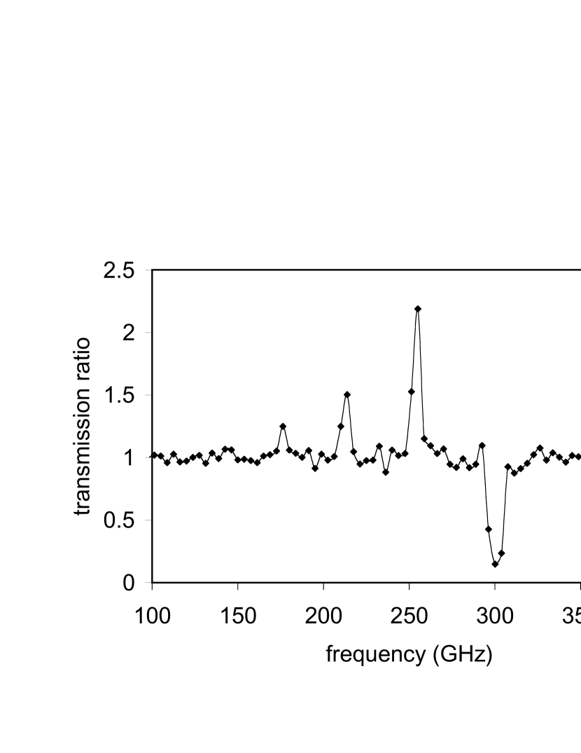
Figure 1: Transmission magnitude at 3 K divided by the transmission magnitude at 15 K. The peaks are due to transitions that are observed at 15 K but are not observed at 3 K because nearly all the clusters are in their ground states.

In Figure 2 we focus on the absorption at 300.6 GHz, which corresponds to the transition from $m=\pm 10$ to $\pm 9$. (The absorption from $m=\pm 9$ to $\pm 8$ has a similar linewidth.) We plot the index of refraction as a function of frequency near this absorption at temperature T = 2.1 K. The index of refraction was calculated directly from the (complex) transmission spectrum using the following equation. The transmission through a slab of thickness $d$ = 1.4 mm with complex index of refraction $\tilde{n}$ is:Ibach

$$\tilde{t}(\omega)=\frac{4\tilde{n}}{(\tilde{n}+1)^{2}}\frac{e^{i\omega\tilde{n}d/c}}{1-(\frac{\tilde{n}-1}{\tilde{n}+1})^{2}e^{2i\omega\tilde{n}d/c}}.$$ (1)

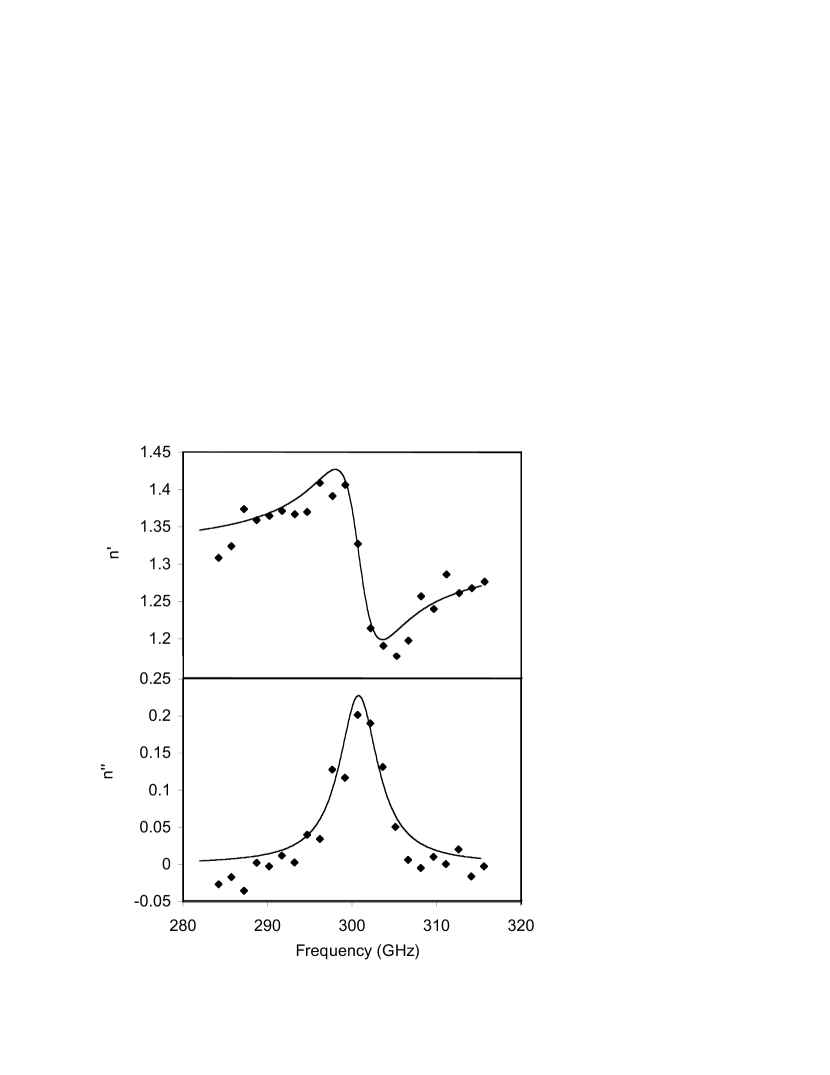
Figure 2: Real and imaginary parts of the index of Mn₁₂-acetate. The index is calculated directly from the transmission using Eq. (1). The line is a fit to Eq. (2).

This equation assumes that all reflections from the interfaces are included, even though THz spectroscopy only collects data within a finite time window after the main pulse. However, in this case the reflectivity is low enough and the absorption is strong enough that the limited time window does not introduce significant error. Notice that since this is a magnetic transition, $n$ must be correctly defined as $\sqrt{\mu\epsilon/\mu_{0}\epsilon_{0}}$, rather than approximated as $\sqrt{\epsilon/\epsilon_{0}}$. We stress that our measurement yields the complex index of refraction without any modeling of either the lineshape or the high and low frequency extrapolations of the response functions.

We model the absorption using the standard form for a magnetic dipole resonance:

$$\mu/\mu_{0}=1+\frac{F\omega_{0}^{2}}{\omega_{0}^{2}-\omega^{2}-i\omega\Gamma}.$$ (2)

We assume that $\epsilon$ is constant over this frequency range. The curve in Figure 2 is a fit to this form, with $\epsilon_{r}\equiv\epsilon/\epsilon_{0}$ = 1.72, $\omega_{0}=300.6$ GHz, $\Gamma=5.5$ GHz, and $F$ = 0.011. The value of $F$ for oriented crystals would be much higher, since the electromagnetic pulse only stimulates transitions in crystals that are oriented with their $c$-axes parallel to the direction of propagation.

Although we have used a standard Lorentzian lineshape with no inhomogeneous broadening to fit these data, it is clear that an equal or better fit could be achieved by considering inhomogeneous broadening. While we can confidently measure the linewidth, we cannot draw any conclusions about the lineshape. However, there has been another measurement of this absorption line by Mukhin et al.Mukhin Their data strongly favor a Gaussian fit to the transmission with a full width at half maximum (FWHM) of 7 GHz.MukhinP (For this material, the FWHM of $ln(|\tilde{t}|)$, $Im(n)$, and $Im(\mu)$ are all approximately equal, so this value can be compared directly to $\Gamma$ in Eq. 2.) The two measured widths are fairly close, but are not equal within the experimental uncertainty. A possible cause of this difference will be discussed later in this paper.

This Gaussian fit is strong evidence for inhomogeneous broadening of the linewidth. However, the cause of this inhomogeneous broadening is unclear. The most obvious source is local magnetic fields, which could be due to the dipolar field of neighboring clusters or the nuclear moments of the manganese atoms. The local dipolar field has not, to our knowledge, been calculated because it depends on the random orientations along the $\pm z$ directions of the magnetic moments of all the other clusters. The calculated value of the hyperfine field varies depending on the type of coupling that is assumed between the electron spins, but its maximum possible value ranges from 270 to 539 G,Hartmann-Boutron96 and its FWHM has been estimated at 280-380 G.Wernsdorfer99

The effect of a local field would be to raise or lower the transition energy between the $\pm 10$ and $\pm 9$ levels, $\Delta E_{10,9}$. From the Hamiltonian, we see that $\Delta E_{10,9}(B)$ = $\Delta E_{10,9}(B=0)\pm\mu_{B}gB_{z}$. For this material, $g$ is very close to 2, so to explain a linewidth of 5.5 GHz requires a magnetic field distribution with width of 0.20 T.

This local field distribution seems to be ruled out by the measurements of the width of the tunneling peak performed by Friedman et al. Friedman98 Starting with a sample cooled in zero applied field, a small magnetic field was applied parallel to the $z$-axis and the relaxation rate of the magnetization toward its equilibrium value was measured. They measured the full width at half maximum to be 236 Oe at 2.6 K. If the local field had a full width at half maximum of 0.20 T, as implied above, then this narrow peak could never have been observed. In addition, the line shape measured by Friedman et al. was clearly Lorentzian. This implies that the inhomogeneous broadening due to local magnetic fields must be significantly smaller than the homogenous effect of lifetime broadening. We note that Friedman et al.’s interpretation of this homogeneous broadening as being due to a lifetime of 250 ps does not imply that Lorentzian tails should be visible in the transitions between $m=\pm 10$ and $m=\pm 9$, since the lifetime of states with larger $|m|$ could be expected to be longer than that of the states involved in tunneling. However, the absence of broadening of Friedman et al.’s data due to local magnetic fields is puzzling.

One possible explanation is that the width measured in tunneling experiments reflects collective effects. The relaxation rate measured by Friedman et al. is a fit to the exponential relaxation that is observed after an initial non-exponential relaxation. As was pointed out in Ref. Prokof ev, , relaxation must actually be a collective process in which the relaxation of one molecule changes the dipole fields of its neighbors, thereby bringing new molecules into resonance. Therefore, it is possible that the width in the relaxation rate would be different from the instantaneous width measured in photon absorption experiments.

In fact, our calculations of the dipolar field show that collective effects must decrease the width of this tunneling peak. Using the atomic positions tabulated in Ref. Lis80, , we calculated the effective field on one cluster due to each of its neighbors. Because the clusters have sizes that are not negligible compared to their separations, this was done by calculating the dipolar field due to the electronic spin of every Mn atom in the neighboring cluster with moment ${\bf m}_{j}=g\mu_{B}S_{j}\hat{\bf z}$, where we choose $S_{j}=+2$ for the eight Mn³⁺ ions and $S_{j}=-3/2$ for the four Mn⁴⁺ ions to reflect their antiferromagnetic coupling. The fields due to all twelve Mn ions located at positions ${\bf r}_{j}$ in the neighboring cluster are summed at the position ${\bf r}_{i}$ of every Mn atom in the cluster under consideration:

$${\bf B}_{i}=\sum_{j}\frac{\mu_{0}}{4\pi}[\frac{3({\bf m}_{j}\cdot{\bf r}_{ij}){\bf r}_{ij}}{r_{ij}^{5}}-\frac{{\bf m}_{j}}{r_{ij}^{3}}],$$ (3)

where ${\bf r}_{ij}$ is the relative position ${\bf r}_{j}-{\bf r}_{i}$. (We assume that the electronic spins are localized on the atomic position, ignoring the actual electronic density.) An effective longitudinal field is then calculated:

$$B_{\rm eff}=\frac{1}{m_{\rm total}}\sum_{i}{\bf B}_{i}\cdot{\bf m}_{i},$$ (4)

where ${\rm m_{total}}=10g\mu_{B}$.

In order to correctly calculate the standard deviation of the dipolar field due to N neighbors exactly, it would be necessary to consider all $2^{N}$ possible arrangements of their spins. However, we can obtain a lower limit on this standard deviation simply by considering the neighboring clusters that contribute the largest fields. As shown in Table 1, there are only 28 neighboring clusters that contribute an effective field greater than 10 G. Assuming there is no ordering of the dipoles, these fields add randomly to give a FWHM of 520 G, as shown in Figure 3. The combination of this field and the hyperfine field is not sufficient to explain the width observed in our spectroscopy. However, we note that it is considerably larger than the width of 236 Oe FWHM observed by Friedman et al., implying that collective effects narrow the observed tunneling width.

Table 1: Fields due to neighboring clusters are calculated using Eqs.  (3) and  (4). All clusters that result in effective fields greater than 10 G are listed. The relative location is given in terms of the unit cell dimensions.

location	field (gauss)
(0,0,$\pm$1)	95.9
($\pm$1,0,0)	56.9
(0,$\pm$1,0)	56.9
($\pm$0.5,$\pm$0.5,$\pm$0.5)	28.4
(0,0,$\pm$2)	19.2
($\pm$0.5,$\pm$0.5,$\pm$1.5)	18.6
($\pm$1,$\pm$1,0)	15.6

Figure 3: Histogram of the distribution of fields resulting from all possible orientations of the neighboring clusters listed in Table 1. The line is a Gaussian with FWHM = 520 G.

One way we could understand the spectroscopy and the tunneling results simultaneously is if there were some source of inhomogeneous broadening other than local magnetic fields. For example, if $\alpha$, the anisotropy constant in the Hamiltonian, varied slightly ($\sim 1\%$) between clusters due to small configurational changes of the ligands surrounding them, then this variation would be seen in the linewidth of the photon-induced transition, but not in the zero field tunneling. The photon absorption experiments would be sensitive to variations in $\alpha$, but the width seen in the zero field tunneling experiments would be due to homogeneous broadening mechanisms, either due to the tunneling time itself or the interactions with phonons, as proposed in Ref. Leuenberger00, . Calculations by Pederson et al. suggest that the arrangement of the ligands is important in determining the anisotropy energy.Pederson99 We note that isomerism of the ligands has been shown to exist in these molecules and results in large variations in the parameters in the Hamiltonian; Aubin97 ; Aubin01 ; Wernsdorfer99 the variations in the ligand positions responsible for the above effect would have to be less dramatic. It is possible that proximity to the isomers could cause neighboring clusters to have some small variation in their Hamiltonians. We also note that recent work of Chudnovsky and Garanin postulates dislocations as the source of spin tunneling and calculates the effect of these dislocations on $\alpha$.Chudnovsky01 The distribution in anisotropy constants calculated in that paper is in very good agreement with the distribution we observe in spectroscopic measurements. It is slightly narrower than the distribution observed by Mukhin et al., but since the density of defects was chosen arbitrarily, this could simply imply that the defect density was higher in the sample measured by Mukhin et al.

Such a distribution of $\alpha$ would have no effect on the width of the relaxation peak in zero field, since in zero field all levels $\pm m$ are degenerate regardless of $\alpha$. However, tunneling peaks at non-zero fields would be broadened, since (neglecting $\beta$) the field $H_{n}=-\alpha n/g\mu_{B}$ that brings the levels $m$ and $-m+n$ into resonance is proportional to $\alpha$. It would be difficult to observe this broadening in tunneling measurements, since the term $\beta S_{z}^{4}$ brings different levels into resonance at different fields, so that if more than one level $m$ is involved in the thermally-assisted tunneling, the relaxation peak will be broadened. However, we note that the width of the relaxation peaks in non-zero fields observed in Ref. Zhong00, is sufficiently large to accommodate the required distribution of $\alpha$.

In conclusion, we measure the linewidth of the single photon transition from $m=\pm 10$ to $m=\pm 9$. This linewidth, while surprisingly large, is in agreement with that observed by Mukhin et al. Mukhin The combination of this linewidth and that measured by Friedman et al. Friedman98 suggests that the anisotropy constant varies between clusters.

We thank A. A. Mukhin for sharing his data and lineshape analysis. This research was supported by Colgate University and by an award from Research Corporation. D. N. H. and G. C. thank the NSF for support.

References

- (1) Jonathan R. Friedman, M.P. Sarachik, J. Tejada, and R. Ziolo, Phys. Rev. Lett. 76, 3830 (1996).
- (2) L. Thomas, F. Lionti, R. Ballou, D. Gatteschi, R. Sessoli, and B. Barbara, Nature 383, 145 (1996).
- (3) Anne Laure Barra, Dante Gatteschi, and Roberta Sessoli, Phys. Rev. B 56, 8192 (1997).
- (4) I. Mirebeau, M. Hennion, H. Casalta, H. Andres, H. U. Güdel, A. V. Irodova, and A. Caneschi, Phys. Rev. Lett. 83, 628 (1999).
- (5) S. Hill, J. A. A. J. Perenboom, N. S. Dalal, T. Hathaway, T. Stalcup, and J. S. Brooks, Phys. Rev. Lett. 80, 2453 (1998).
- (6) A. Fort, A. Rettori, J. Villain, D. Gatteschi, and R. Sessoli, Phys. Rev. Lett. 80, 612 (1998).
- (7) Fernando Luis, Juan Bartolomé, and Julio F. Fernández, Phys. Rev. B 57, 505 (1998).
- (8) W. Bao, R. A. Robinson, J. R. Friedman, H. Casalta, E. Rumberger, and D. N. Hendrickson, cond-mat/0008042.
- (9) A. A. Mukhin, V. D. Travkin, A. K. Zvezdin, A. Caneschi, D. Gatteschi, and R. Sessoli, Physica B, 284-288, 1221 (2000) and A. A. Mukhin, V. D. Travkin, A. K. Zvezdin, S. P. Lebedev, A. Caneschi, and D. Gatteschi, Europhys. Lett. 44, 778 (1998).
- (10) Yicheng Zhong, M. P. Sarachik, Jonathan R. Friedman, R. A. Robinson, T. M. Kelley, H. Nakotte, A. C. Christianson, F. Trouw, S. M. J. Aubin, and D. N. Hendrickson, J. of Appl. Phys. 85, 5636 (1999).
- (11) T. Lis, Acta Crystallogr. B 36, 2042 (1980).
- (12) H. Ibach and H. Lüth, Solid-State Physics, (Springer, Berlin, 1995), p. 291.
- (13) A. Mukhin, B. Gorshunov, M. Dressel, C. Sangregorio, and D. Gatteschi, Phys. Rev. B 63, 214411 (2001), and A. Mukhin, private communication.
- (14) Françoise Hartmann-Boutron, Paolo Politi, and Jacques Villain, Int. J. of Mod. Phys. B 10, 2577 (1996).
- (15) W. Wernsdorfer, R. Sessoli, and D. Gatteschi, Europhys. Lett. 47, 254 (1999).
- (16) Jonathan R. Friedman, M. P. Sarachik, and R. Ziolo, Phys. Rev. B 58, R14729, (1998).
- (17) N. V. Prokofev and P. C. E. Stamp, Phys. Rev. Lett. 80, 5794 (1998).
- (18) Michael N. Leuenberger and Daniel Loss, Phys. Rev. B 61, 1286 (2000).
- (19) M. R. Pederson and S. N. Khanna, Phys. Rev. B 60, 9566 (1999).
- (20) S. M. J. Aubin, Ziming Sun, Ilia A. Guzei, Arnold L. Rheingold, George Christou, and David N. Hendrickson, Chem. Commun., 2239 (1997).
- (21) Sheila M. J. Aubin, Ziming Sun, Hilary J. Eppley, Evan M. Rumberger, Ilia A. Guzei, Kirsten Folting, Peter K. Gantzel, Arnold L. Rheingold, George Christou, and David N. Hendrickson, Inorganic Chemistry, 40, 2127 (2001).
- (22) E. M. Chudnovsky and D. A. Garanin, cond-mat/0105195 and cond-mat/0105518.
- (23) Yicheng Zhong, M.P. Sarachik, Jae Yoo, and D. N. Hendrickson, Phys. Rev. B 62, R9256 (2000).