[cond-mat/0110655] 1 ℱ⁢(𝑥_Δ) is plotted against the variable 𝑥_Δ, for 𝑛=2⁢𝑚. There is very good agreement with the analytical results, improving as 𝑚 increases, as expected for an asymptotic result.

Random matrix theory for the analysis of the performance of an analog computer: a scaling theory

Asa Ben-Hur^a, Joshua Feinberg^b,c, Shmuel Fishman^c,d
& Hava T. Siegelmann^e

^a)Biochemistry Department,

Stanford University, CA 94305, USA

^b)Physics Department,

University of Haifa at Oranim, Tivon 36006, Israel

^c)Physics Department,

Technion, Israel Institute of Technology, Haifa 32000, Israel

^d)Institute for Theoretical Physics

University of California

Santa Barbara, CA 93106, USA

^e)Bio-Computation Laboratory,

Department of Computer Science, University of Massachusetts,

Amherst MA 01003

PACS numbers: 5.45-a, 89.79+c, 89.75.D

An analog computer is a physical device that performs computation, evolving in continuous time and phase space; its evolution in phase space can be modeled by dynamical systems (DS) [1], the way classical systems such as particles moving in a potential (or electric circuits), are modeled. This description makes a large set of analytical tools and physical intuition, developed for dynamical systems, applicable to the analysis of analog computers. In contrast, the evolution of a digital computer is described by a dynamical system, discrete both in its phase space and in time. The most relevant examples of analog computers are VLSI devices implementing neural networks [2], or neuromorphic systems [3], whose structure is directly motivated by the workings of the brain. Various processes taking place in living cells can be considered as analog computation [4]. Dynamical systems (described by ordinary differential equations) are also used to solve computational problems [5, 6, 7]. The standard theory of computation and computational complexity [8] deals with computation in discrete time and phase space, and is inadequate for the description of such systems. For the analysis of computation by analog devices a theory that is valid in continuous time and phase space is required. Since the systems in question are physical systems, the computation time is the time required for a system to reach the vicinity of an attractor (a stable fixed point in the present work) combined with the time required to verify that it indeed reached this vicinity. This time is the elapsed time measured by a clock, contrary to standard computation theory, where it is the number of steps.

In the exploration of physical systems, it is sometimes much easier to study statistical ensembles of systems, estimating their typical behavior using statistical methods [9, 10, 11]. Ensembles of systems modeling the dynamics of populations were studied as well [12, 13]. The statistical theories describe many general features of the problems that are inverstigated, but specific systems require special attention [10, 13]. In this letter a statistical theory is used to calculate the computational complexity of a standard representative problem, namely Linear Programming (LP), as solved by a DS. A detailed version was published in the computer science literature [14].

In two recent papers we have proposed a framework for computing with DS that converge exponentially to fixed points [15]. For such systems it is natural to consider the attracting fixed point as the output. The input can be modeled in various ways. One possible choice is the initial condition. This is appropriate when the aim of the computation is to decide to which attractor out of many possible ones the system flows [16]. Here, as in [15], the parameters on which the system of DS depends (e.g., the parameters appearing in the vector field $F$ in (1)) are the input.

The basic entity of the computational model is a dynamical system [1], that may be defined by a set of Ordinary Differential Equations (ODEs)

\frac{dx}{dt}=F(x),

(1)

where $x$ is an $n$ -dimensional vector, and $F$ is an $n$ -dimensional smooth vector field, which converges exponentially to a fixed point. Eq. (1) solves a computational problem as follows: Given an instance of the problem, the parameters of the vector field $F$ are set, and it is started from some pre-determined initial condition. The result of the computation is then deduced from the fixed point that the system approaches.

In our model we assume we have a physical implementation of the flow equation (1). Thus, the vector field $F$ need not be computed, and the computation time is determined by the convergence time to the attractive fixed point. In other words, the time of flow to the vicinity of the attractor is a good measure of complexity, namely the computational effort, for the class of continuous dynamical systems introduced above [15].

In this letter we will consider real inputs, as the ones found in physical experiments, and that are studied in the BSS model [17]. For computational models defined on the real numbers, worst case behavior, that is traditionally studied in computer science, can be ill defined and lead to infinite computation times, in particular, for some methods for solving LP [17, 18]. Therefore, we compute the distribution of computation times for a probabilistic model of LP instances with Gaussian distribution of the data like in [19, 20]. Ill-defined instances constitute a set of zero measure in our probability ensemble, and need not be concerned about.

The computational complexity of the method presented here is ${\cal O}(n\log n)$ , compared to ${\cal O}(n^{3.5}\log n)$ found for standard interior point methods [21]. The basic reason is that for standard methods (such as interior point methods), the major component of the complexity of each iteration is ${\cal O}(n^{3})$ due to matrix decomposition and inversion of the constraint matrix, while here, because of its analog nature, the system just flows according to its equations of motion (which need not be computed).

Since we consider the evolution of a vector filed, our model is inherently parallel. Therefore, to make the analog vs. digital comparison entirely fair, we should compare the complexity of our method to that of the best parallel algorithm. The latter can reduce the ${\cal O}(n^{3})$ time needed for matrix decomposition/inversion to polylogarithmic time (for well-posed problems), at the cost of ${\cal O}(n^{2.5})$ processors [22], while our system of equations (1) uses only ${\cal O}(n)$ variables.

Linear programming is a P-complete problem [8], i.e. it is representative of all problems that can be solved in polynomial time. The standard form of LP is to find

\max\{c^{T}x~{}:~{}x\in{{{\rm I\mkern-3.5muR}}}^{n},Ax=b,x\geq 0\}

(2)

where $c\in{{{\rm I\mkern-3.5muR}}}^{n},b\in{{{\rm I\mkern-3.5muR}}}^{m},A\in{{{\rm I\mkern-3.5muR}}}^{m\times n}$ and $m\leq n$ . The set generated by the constraints in (2) is a polyheder. If a bounded optimal solution exists, it is obtained at one of its vertices. The vector defining this optimal vertex can be decomposed (in an appropriate basis) in the form $x=(x_{{\cal N}},x_{{\cal B}})$ where $x_{\cal N}=0$ is an $n-m$ component vector, while $x_{\cal B}=B^{-1}b\geq 0$ is an $m$ component vector, and $B$ is the $m\times m$ matrix whose columns are the columns of $A$ with indices identical to the ones of $x_{\cal B}$ . Similarly, we decompose $A=(N,B)$ .

A flow of the form (1) converging to the optimal vertex, introduced by Faybusovich [6] will be studied here. Its vector field $F$ is a projection of the gradient of the cost function $c^{T}x$ onto the constraint set, relative to a Riemannian metric which enforces the positivity constraints $x\geq 0$ [6]. It is given by

F(x)=[X-XA^{T}(AXA^{T})^{-1}AX]\>c\;,

(3)

where $X$ is the diagonal matrix $\mbox{Diag}(x_{1}\dots x_{n})$ . The $nm+n$ entries of $A$ and $c$ , namely, the parameters of the vector field $F$ , constitute the input; as in other models of computation, we ignore the time it takes to “load” the input, since this step does not reflect the complexity of the computation being performed, either in analog or digital computation. It was shown in [23] that the flow equations given by (1) and (3) are, in fact, part of a system of Hamiltonian equations of motion of a completely integrable system of a Toda type. Therefore, like the Toda system, it is integrable with the formal solution [6]

x_{i}(t)=x_{i}(0)\exp\left(-\Delta_{i}t+\sum_{j=1}^{m}\alpha_{ji}\log\frac{x_{j+n-m}(t)}{x_{j+n-m}(0)}\right)

(4)

( $i=1,\ldots,n-m$ ), that describes the time evolution of the $n-m$ independent variables $x_{\cal N}(t)$ , in terms of the variables $x_{\cal B}(t)$ . In (4) $x_{i}(0)$ and $x_{j+n-m}(0)$ are components of the initial condition, $x_{j+n-m}(t)$ are the $x_{{\cal B}}$ components of the solution, $\alpha_{ji}=-(B^{-1}N)_{ji}$ is an $m\times(n-m)$ matrix, while

\Delta_{i}=-c_{i}-\sum_{j=1}^{m}c_{j}\alpha_{ji}\,.

(5)

For the decomposition $x=(x_{{\cal N}},x_{{\cal B}})$ used for the optimal vertex $\Delta_{i}\geq 0~{}~{}i=1,\ldots,n-m\,,$ and $x_{\cal N}(t)$ converges to 0, while $x_{\cal B}(t)$ converges to $x^{*}=B^{-1}b$ . Note that the analytical solution is only a formal one, and does not provide an answer to the LP instance, since the $\Delta_{i}$ depend on the partition of $A$ , and only relative to a partition corresponding to a maximum vertex are all the $\Delta_{i}$ positive.

The second term in (4), when it is positive, is a kind of “barrier”: $\Delta_{i}t$ must be larger than the barrier before $x_{i}$ can decrease to zero. In the following we ignore the contribution of the initial condition and denote the value of this term in the infinite time limit by

\beta_{i}=\sum_{j=1}^{m}\alpha_{ji}\log x_{j+n-m}^{*}.

(6)

Note that although one of the $x_{j}^{*}$ may vanish, in the probabilistic ensemble studied here such an event is of measure zero and therefore should not be considered. In order for $x(t)$ to be close to the maximum vertex we must have $x_{i}(t)<\epsilon$ for $i=1,\ldots,n-m$ for some small positive $\epsilon$ , namely $\exp(-\Delta_{i}t+\beta_{i})<\epsilon~{},~{}~{}\mbox{for}~{}i=1,\ldots,n-m.$ Therefore we consider

T=\max_{i}\left(\frac{\beta_{i}}{\Delta_{i}}+\frac{|\log\epsilon|}{\Delta_{i}}\right)~{},

(7)

as the computation time. We denote

\Delta_{\min}=\min_{i}\Delta_{i},~{}~{}~{}\beta_{\max}=\max_{i}\beta_{i}\;.

(8)

The $\Delta_{i}$ can be arbitrarily small when the inputs are real numbers, but in the probabilistic model, “bad” instances are rare as is clear from (10).

The ensemble we analyze consists of LP problems in which the components of $(A,b,c)$ are independent identically distributed (i.i.d.) random variables taken from the standard Gaussian distribution with 0 mean and unit variance. With the introduction of a probabilistic model of LP instances, $\Delta_{\min},\,\beta_{\max}$ and $T$ become random variables. Since the expression for $\Delta_{i}$ , equation (5), is independent of $b$ , its distribution is independent of $b$ . For a given realization of $A$ and $c$ , with a partition of $A$ into $(N,B)$ such that $\Delta_{i}\geq 0$ , there exists a vector $b$ such that the resulting polyheder has a bounded optimal solution. Since $b$ in our probabilistic model is independent of $A$ we obtain:
${\cal P}(\Delta_{\min}<\Delta|\Delta_{\min}>0,\mbox{LP instance has a bounded maximum vertex})={\cal P}(\Delta_{\min}<\Delta|\Delta_{\min}>0)$ .

We wish to compute the probability distribution of $\Delta_{\min}$ for instances with a bounded solution, when $\Delta_{\min}>0$ , denoted by ${\cal P}(\Delta_{min}>\Delta|\Delta_{min}>0)$ . It turns out that it is much easier to analytically calculate the probability distribution of $\Delta_{min}$ for a given partition of the matrix $A$ . In the probabilistic model we defined, ${\cal P}(\Delta_{\min}>\Delta|\Delta_{\min}>0)$ is proportional to the probability that $\Delta_{\min}>\Delta$ for a fixed partition (9). Let the index 1 stand for the partition where $B$ is taken from the last $m$ columns of $A$ . In [14] we proved, using the symmetry resulting from the identity of the Gaussian variables, that

{\cal P}(\Delta_{\min}>\Delta|\Delta_{\min}>0)=\frac{{\cal P}(\Delta_{min1}>\Delta)}{{\cal P}(\Delta_{min1}>0)}

(9)

for $\Delta>0$ , where $\Delta_{min1}=\min\{\Delta_{i}~{}|~{}\Delta_{i}\mbox{~{}are computed relative to the partition 1}\}\,$ and ${\cal P}(\Delta_{min1}>0)=1/2^{n-m}\;$ .

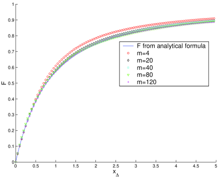
Integrating over the Gaussian variables of the ensemble, the probability ${\cal P}(\Delta_{min1}>\Delta)$ was computed in [14] for a specific partition of $A$ in the large $(n,m)$ asymptotic limit, making use of methods of random matrix theory. Given ${\cal P}(\Delta_{min1}>\Delta)$ , then ${\cal P}(\Delta_{\min}>\Delta|\Delta_{\min}>0)$ is obtained with the help of (9). In the large $(n,m)$ limit the probability ${\cal P}(\Delta_{min}<\Delta|\Delta_{min}>0)\equiv{\cal F}^{(n,m)}(\Delta)$ is of the scaling form

{\cal F}^{(n,m)}(\Delta)=1-e^{x_{\Delta}^{2}}\,{\rm erfc}(x_{\Delta})\ \equiv{\cal F}(x_{\Delta}).

(10)

with the scaling variable $x_{\Delta}(n,m)={1\over\sqrt{\pi}}\left({n\over m}-1\right)\,\sqrt{m}\Delta\,.$ The scaling function ${\cal F}$ contains all asymptotic information on $\Delta$ . The distribution ${\cal F}(x_{\Delta})$ is very wide and does not have a mean. Also the average of $1/x_{\Delta}$ diverges.

In order to the demonstrate this result numerically, we generated LP instances where $(A,b,c)$ are random Gaussian variables and solved for them the LP problem with the IMSL C library. We obtained an estimate of ${\cal F}^{(n,m)}(\Delta)={\cal P}(\Delta_{min}<\Delta|\Delta_{min}>0)$ , and of the corresponding cumulative distribution functions of the barrier $\beta_{\max}$ and $T$ . In Fig. 1 the numerical results are compared with the analytical formula (10).

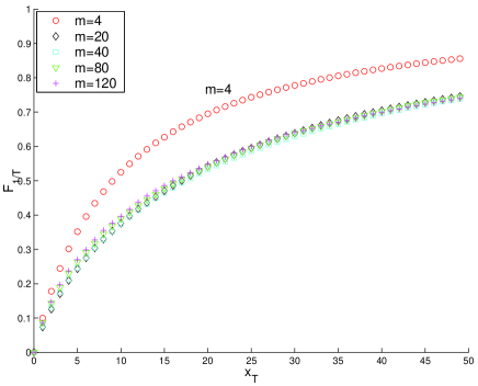
Refer to caption — Figure 1: ${\cal F}(x_{\Delta})$ is plotted against the variable $x_{\Delta}$ , for $n=2m$ . There is very good agreement with the analytical results, improving as $m$ increases, as expected for an asymptotic result.

The existence of scaling functions like (10) for the barrier $\beta_{max}$ , that is the maximum of the $\beta_{i}$ defined by (6) and for $T$ defined by (7) was verified numerically (see Fig. 2 for $T$ ). In particular for fixed $m/n$ , we found that

{\cal P}(1/\beta_{max}~{}<~{}1/\beta)\equiv{\cal F}^{(n,m)}_{1/\beta_{max}}(1/\beta)={\cal F}_{1/{\beta_{max}}}(x_{\beta})

(11)

and

{\cal P}(1/T~{}<~{}1/t)\equiv{\cal F}^{(n,m)}_{1/T}(1/t)={\cal F}_{1/T}(x_{T}).

(12)

The scaling variables are $x_{\beta}\sim m/\beta$ and $x_{T}\sim m\log m/t$ .

The scaling functions (10), (11) and (12) imply the asymptotic behavior

\displaystyle 1/\Delta_{\min}\sim\sqrt{m},~{}~{}~{}~{}\beta_{\max}\sim m,~{}~{}~{}T\sim m\log m

(13)

with “high probability” [14].

In this letter we computed the problem size dependence of the distributions of quantities that govern the convergence of a DS that solves the LP problem [6]. To the best of our knowledge, this is the first time such distributions are computed. In particular, knowledge of the distribution functions enables to obtain the “high probability” behavior (13), and the moments (if these exist). The main result of the present work is that the distribution functions of the convergence rate, $\Delta_{min}$ , the barrier $\beta_{max}$ and the computation time $T$ are scaling functions; i.e., in the asymptotic limit of large $(n,m)$ , each depends on the problem size only through a scaling variable. In other words these are not arbitrary functions of the three variables, but each is a function only of one variable, $x_{\Delta}$ , $x_{\beta}$ or $x_{T}$ . The distribution function of $\Delta_{min}$ was calculated analytically, and the result was verified numerically. The scaling functions, even if known only numerically, can be useful for the understanding of the behavior for large values of $(n,m)$ that are beyond the limits of numerical simulations.

In this letter the distribution functions of various quantities that characterize the computational complexity, were found to be scaling functions in the large $(n,m)$ limit. This is analogous to the situation found for the central limit theorem, for critical phenomena [24] and for Anderson localization [25], in spite of the very different nature of these problems. It is demonstrated here how for the implementation of the LP problem on a physical device, methods used in theoretical physics enable to describe the distribution of computation times in a simple and physically transparent form. Based on our experience with certain universality properties of rectangular and chiral random matrix models [26], we expect some universality for computational problems, that should be explored. The obvious questions are: Is the Gaussian nature of the ensemble unimportant in analogy with [26]? Are there universality classes [24] of analog computational problems, and if they exist, what are they? Are these analogous to the classification of [13]? We believe it can be instructive to explore computational problems using methodologies of theoretical physics as was demonstrated here for linear programming.

Acknowledgements: It is our great pleasure to thank Arkadi Nemirovski, Eduardo Sontag and Ofer Zeitouni for stimulating and informative discussions. We thank a referee for bringing [12, 13] to our attention. This research was supported in part by the US-Israel Binational Science Foundation (BSF), by the Israeli Science Foundation, by the US National Science Foundation under Grant No. PHY99-07949 and by the Minerva Center of Nonlinear Physics of Complex Systems.

References

[1] E. Ott, Chaos in Dynamical Systems. Cambridge University Press, Cambridge, England, 1993.
[2] J. Hertz, A. Krogh, and R. Palmer. Introduction to the Theory of Neural Computation. Addison-Wesley, Redwood City, 1991.
[3] C. Mead. Analog VLSI and Neural Systems. Addison-Wesley, 1989.
[4] D. Bray. Nature 376, 307 (1995); A. Ben-Hur and H.T. Siegelmann. Proceedings of MCU 2001, Lecture Notes in Computer Science 2055, pages 11-24, M. Margenstern and Y. Rogozhin (Editors), Springer Verlag, Berlin 2001 (and references therein).
[5] R. W. Brockett. Linear Algebra and Its Applications 146, 79 (1991); M.S. Branicky. Analog computation with continuous ODEs. In Proceedings of the IEEE Workshop on Physics and Computation , pages 265–274, Dallas, TX, 1994.
[6] L. Faybusovich. IMA Journal of Mathematical Control and Information 8, 135 (1991).
[7] U. Helmke and J.B. Moore. Optimization and Dynamical Systems. Springer Verlag, London, 1994.
[8] C. Papadimitriou. Computational Complexity. Addison-Wesley, Reading, Mass., 1995.
[9] M.L. Mehta. Random Matrices (2nd ed.). Academic Press, San-Diego, CA, 1991.
[10] T.A. Brody, J. Flores, J.B. French, P.A. Mello, A. Pandey and S.S.M. Wong. Rev. Mod. Phys. 53, 385 (1981).
[11] O. Bohigas, M.-J. Giannoni and C. Schmit. Phys. Rev. Lett. 52, 1 (1984); O. Bohigas. Random Matrix Theories and Chaotic Dynamics. In Chaos and Quantum Physics, Proceedings of the Les-Houches Summer School, Session LII, 1989, M.-J. Giannoni, A. Voros and J. Zinn-Justin, (eds.), North-Holland, Amsterdam, The Netherlands, 1991.
[12] R. M. May, Nature 238, 413 (1972); M. R. Gardner and W. R. Ashby, Nature 228, 784 (1970).
[13] A. Roberts, Nature 251, 607 (1974); M. E. Gilpin, Nature 254, 137 (1975); R. E. McMurtrie, J. Theor. Biol. 50, 1 (1975); T. Hogg, B. A. Huberman and J. M. McGlade, Proc. Roy. Soc. Lond. B 237, 43 (1989).
[14] A. Ben-Hur, J. Feinberg S. Fishman, and H.T. Siegelmann, J. Complexity 19, 474 (2003) (preprint cs.CC/0110056).
[15] H.T. Siegelmann, A. Ben-Hur and S. Fishman, Phys. Rev. Lett. 83, 1463 (1999); A. Ben-Hur, H.T. Siegelmann, and S. Fishman. J. Complexity 18, 51 (2002).
[16] H.T. Siegelmann and S. Fishman. Physica 120, 214 (1998).
[17] L. Blum, F. Cucker, M. Shub, and S. Smale. Complexity and real Computation. Springer-Verlag, 1999.
[18] S. Smale. Math. Programming 27, 241 (1983); M.J. Todd. Mathematics of Operations Research 16, 671 (1991).
[19] S. Smale. Math. Programming 27, 241 (1983).
M.J. Todd. Mathematics of Operations Research 16, 671 (1991).
[20] R. Shamir. Management Science 33(3), 301 (1987).
[21] Y. Ye. Interior Point Algorithms: Theory and Analysis. John Wiley and Sons Inc., 1997.
[22] V. Y. Pan and J. Reif, Computers and Mathematics (with Applications) 17, 1481 (1989).
[23] L. Faybusovich. Physica D53, 217 (1991).
[24] K.G. Wilson and J. Kogut, Phys. Rep. 12, (1974) 75.
[25] E. Abrahams, P. W. Anderson, D. C. Licciardelo and T. V. Ramakrishnan, Phys. Rev. Lett. 42 (1979) 673.
[26] Some papers that treat random real rectangular matrices, such as the matrices relevant for this work (which are not necessarily Gaussian ), are: A. Anderson, R. C. Myers and V. Periwal, Phys. Lett.B 254, 89 (1991); Nucl. Phys. B 360, (1991) 463 (Section 3); J. Feinberg and A. Zee, J. Stat. Mech. 87, 473 (1997); For earlier work see: G.M. Cicuta, L. Molinari, E. Montaldi and F. Riva, J. Math.Phys. 28, 1716 (1987).