Monte Carlo simulation of electromigration phenomena in metallic lines

Abstract

The electromigration (EM) of metallic lines is studied in terms of competition between two percolative processes taking place in a random resistor network. The effects associated with the transport of mass and with the consequent growth of the internal stress are accounted for by stochastic generation and recovery of voids, driven by the external current. Monte Carlo simulations enable us to investigate within a unified theoretical framework a variety of relevant aspects of EM degradation as: damage patterns, the distribution of the time to failures, early stage resistance change in the presence of compositional effects, Black’s law, geometrical effects, etc. A general agreement is found with the experimental findings.

1 Introduction

In recent times, the study of breakdown phenomena in electrical devices has received a lot of attention, mainly for the increasing level of miniaturization which makes failure problems more and more crucial [1]. Failure occurs in many cases by the degradation of metallic interconnects (thin films) which, because of electromigration (EM), lose their conducting properties. EM arises from the transport of matter at the atomic level driven by a high current density [1, 2, 3]. More precisely, the damage, consisting in the formation and growth of voids and hillocks in different regions of the film, is due to a non-steady atomic trasport associated with a nonvanishing divergence of the atomic flux. A fundamental ingredient in the description of the EM damage of the interconnects in electronic devices is represented by the granular structure of the materials employed, Al, Cu, Al alloys, etc. In fact, it has been observed [1, 2, 3] that the atomic transport through the grain boundaries (transport channels) far exceeds that through the grain bulks. Therefore, it is generally possible to neglect mass transport everywhere except within these channels and to describe the film as an interconnected grain boundary network [1]. Futhermore, a high degree of disorder is usually present in alloy films due to compositional effects (CE) and to thermal gradients [1, 2, 3]. Finally, it must be underlined the rôle of mechanical stress. Indeed, the depletion and accumulation of mass in different regions of the film, implies also the growth of mechanical stress, which contrasts the atomic flux due to EM [1, 2, 4]. On the basis of the above description, we have developed a model which describes the EM damage of interconnects in terms of two competing biased percolations taking place in a Random Resistor Network (RRN) [5]. Monte Carlo simulations allow us to explore a variety of relevant aspects of EM degradation as: damage patterns, the distribution of the time to failures, early stage resistance change in the presence of compositional effects, Black’s law, geometrical effects, etc. The paper is organized as follows. Section 2 describes the model used and the numerical procedure of simulations. Section 3 reports the results and compares theory with well accepted phenomenological behaviors. Major conclusions are drawn in Sec. 4.

2 Model

A metallic line of length $L$ and width $w$ is described as a two-dimensional rectangular-lattice network of regular resistors, $r_{reg}$. The network lies on an insulating substrate at temperature $T_{0}$ acting as a thermal reservoir. The total number of elementary resistors in the network is given by: $N_{tot}=2N_{L}N_{w}+N_{L}-N_{w}$, where $N_{L}$ and $N_{w}$ determine the length and the width of the network. To reduce the computational efforts, long lines are simulated by assuming that only a portion of the line is responsible of the resistance variations. The network represents this portion and its length is taken $1/F$ times smaller than the line length. Thus, the relative resistance variation of the whole line is obtained by multiplying the relative resistance variations of the network by the factor $F$. The resistance of the $n$-th resistor depends on temperature according with:

$$r_{reg,n}(T_{n})=r_{ref}[1+\alpha(T_{n}-T_{ref})]$$ (1)

where $\alpha$ is the temperature coefficient of resistance (TCR), $T_{n}$ is the local temperature, $T_{ref}$ and $r_{ref}$ are the reference values for the TCR. The network is contacted at the left and right hand sides to perfectly conducting bars through which a constant stress current $I$ is applied. The Joule heating induced by $I$ is taken into account by defining $T_{n}$ as [6]:

$$T_{n}=T_{0}+A\Bigl{[}r_{n}i_{n}^{2}+{B\over N_{neig}}\sum_{m=1}^{N_{neig}}\Bigl{(}r_{m,n}i_{m,n}^{2}-r_{n}i_{n}^{2}\Bigr{)}\Bigr{]},$$ (2)

where $A$ is the thermal resistance of the single resistor and $N_{neig}$ the number of first neighbours of the $n$-th resistor. The value $B=3/4$ is chosen to provide a uniform heating for the perfect network [6]. By taking this expression we are assuming an istantaneous thermalization. In the presence of a current stress, the EM damage is simulated by allowing the breaking of regular resistors, i.e. by replacing $r_{reg}\rightarrow r_{OP}$, $r_{OP}=10^{9}\ r_{ref}$. We remark that $r_{OP}$ represents an open circuit (OP) associated with the formation of voids inside the line. Simultaneously, a recovery process which allows the healing of the broken resistors, is also considered. The complete failure of the line is thus associated with the existence of at least one continuous path of OP between the upper and lower sides of the network (percolation threshold) [5]. The probability $W_{OP}$ for the $n$-th resistor to become OP is taken as:

$$W_{OP}=\exp(-{E_{OP}/k_{B}T_{n}})$$ (3)

where $E_{OP}$ is a characteristic activation energy and $k_{B}$ the Boltzmann constant. A similar expression is taken for the recovery process probability $W_{RE}$, with $E_{OP}$ replaced by $E_{RE}$. Accordingly, the elimination of resistors represents the mass transport due to an electron wind, and the recovery of resistors, the back-up flow of atoms due to the mechanical stress. The two activation energies control the competition between these two opposite processes.

2.1 Compositional effects (CE)

In Al alloys (Al-Cu, Al-Si) CE are observed at the early stages of EM test of metallic lines. Here, we limit ourself to study the CE due to: (i) a sample heating, (ii) an intrinsic defectiveness of the manifactured samples. To simulate the CE induced by heating, we take into account the actual thermal treatment undergone by the lines just before the EM test. Here, we consider one specific EM experiment which is performed with standard techniques on Al-0.5%Cu lines. For these lines, the last thermal treatment occurred during fabrication was a high temperature annealing followed by a rapid cooling. This treatment left a non-equilibrium concentration of Cu dissolved into the Al matrix. Therefore, in the early stage of the EM test, the heating associated with the stress conditions allows a relaxation toward the equilibrium concentration of the Cu atoms and gives rise to the formation of CuAl₂ precipitates. The variation of the line composition is simulated by changing, with probability $W_{ri}$, the resistance of the $n$-th resistor from $r_{reg}$ to $r_{imp}$ (impurity resistors), where we take:

$$W_{ri}={\rm exp}(-{E_{ri}/k_{B}T_{n}})$$ (4)

being $E_{ri}$ an activation energy characterizing this process. The mechanism of Cu dissolution into the Al matrix, antagonist to the precipitation, is simultaneously considered by taking a similar expression for the probability of the reverse process $r_{imp}\rightarrow r_{reg}$, which is determined by an activation energy $E_{ir}$. As a consequence of the two competing processes, a steady state concentration of $r_{imp}$ is achieved on a time scale much shorter than that of EM. The intrinsic defectiveness of the samples manifests itself by the existence of samples of the same material and geometry but with drastically different failure times. To simulate this second case of CE, we have considered the evolution of networks with different initial concentration $p_{ini}$ of OP resistors. Accordingly, we have assumed $p_{ini}$ randomly distributed, and chosen values of $r_{0}$ in such a way to keep nearly the same resistance value of similar undefected samples.

2.2 Numerical procedure

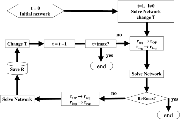
Figure 1: Flowchart of the Monte Carlo simulator.

The network evolution is obtained by Monte Carlo simulations which are carried out according with the flowchart shown in Fig. 1. (i) Starting from the initial network, we calculate $i_{n}$ and the network resistance $R$ by solving Kirchhoff’s loop equations. Moreover, we calculate $T_{n}$ by using Eq. (2). (ii) OP and $r_{imp}$ are generated with the corresponding probabilities $W_{OP}$ and $W_{ri}$, while the remaining $r_{reg}$ are changed according to $T_{n}$. Then, $i_{n}$ and $T_{n}$ are recalculated. (iii) OP and $r_{imp}$ are recovered. (iv) $i_{n}$, $T_{n}$ and $R$ are recalculated. This procedure is iterated from (ii), thus the loop (ii)-(iv) corresponds to an iteration step, which is associated with a unit time step on an arbitrary time scale to be calibrated by comparison with experiments. The iteration proceeds until, depending on the values of the model parameters, the following two possibilities are achieved: irreversible failure or steady-state evolution. The irreversible failure can be established by a criterion for the increase of resistance over its initial value as suggested by experiments (typically of 20 %).

3 Results

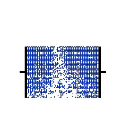
Figure 2: Simulated damage pattern at the complete failure of a network $40\times 40$ by using the parameters specified in the text.

To check the ability of the model to describe EM experiments, simulations are performed on Al-0.5%Cu lines [7]. A significant aspect related to the electrical failure is the damage pattern, which evidences the correlations among different failing regions just before the complete failure. Figure 2 reports a typical damaged pattern obtained for a network of sizes $40\times 40$ with the following parameters chosen according to the experimental conditions of Ref. [7]: $I=1.1\times 10^{-2}\ A$, $T_{0}=219\ ^{o}C$, $T_{ref}=0\ ^{o}C$, $r_{ref}=296\ \Omega$, $\alpha=3.6\times 10^{-3}\ {}^{o}C^{-1}$. To provide for an initial heating of the network of about 15 ${}^{o}C$, the value of the thermal resistance $A$ is taken as: $1.5\times 10^{6}\ {}^{o}C/W$; to account for an initial defectiveness of the line we take $p_{ini}\ \approx\ 0.01$. Moreover, to save computational time, we choose F=30 and for the activation energies responsible of EM we use values smaller than those found in experiments, as: $E_{OP}$ = $E_{RE}$ = 0.43 eV. We have tested that, by scaling the value of $E_{OP}$ in the range $0.2\div 0.6$ eV, the median time to failure (MTF) changes over more than two orders of magnitude while its relative standard deviation remains constant within a factor of two. Consistently with this choice, to account for the different characteristic times of the two processes, also the activation energies responsible of CE have been reduced: we take $E_{ri}=0.22\ eV$ and $E_{ir}$=0.17 eV. Moreover, for the impurity resistor we use $r_{imp}=350\ \Omega$. We note that the damage pattern in Fig. 2 well reproduces the experimental pattern observed by SEM in metallic lines [1, 3].

Figure 3: Simulation of the relative variations of resistance as function of time for Al-0.5%Cu lines. The insert shows enlarged CE in the early stage of EM.

Figure 4: Simulation of the relative variations of resistance as function of time corresponding to networks with different initial defectiveness and comparable resistance. Continuous curves represent evolutions obtained by taking $p_{ini}\approx 0.1$, the dotted curves are for $p_{ini}\approx 0.3$. The insert reports a set of experimental results performed on samples with the same geometry and comparable resistance.

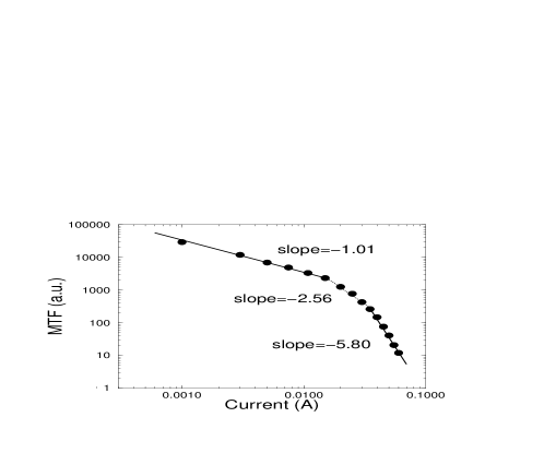
Figure 5: Median time to failure as a function of stressing current for a rectangular network $12\times 400$ with the parameter values specified in the text. The slopes in the relevant regions of the curve (low, moderate, and high current stresses) are reported in the figure.

The results of simulation for the resistance evolutions are reported in Fig.3. All the parameters are the same used for Fig. 2, except for the network sizes, that are now $N_{L}=N_{w}=70$. The insert shows the early stage resistance decrease due to the thermal CE. The simulations reproduce satisfactorily the experimental evidence of both the early stage and the pre-failure regime of the resistance evolution [7]. To investigate the rôle of the intrinsic defectiveness of the line, we have simulated the evolution of the network with a different initial concentration of OP resistors randomly distributed. Moreover, we have chosen $r_{ref}\ =\ 229\ \Omega$ to have nearly the same resistance of the networks considered in Fig. 3. We report in Fig. 4 the relative variations of the resistance as function of time for the two sets of simulations: continuous curves are the same of Fig. 3 ($p_{ini}\approx 0.1$), the other ones corresponding to $p_{ini}\approx 0.3$. We show in the insert the results of the experiments [7] performed on samples with the same geometry and comparable resistance but exhibiting completely different failure times. The simulations well reproduce the experiments [7].

EM tests are performed in the so-called “accelerate conditions”, i.e. the current density, $J$, and the stress temperature, $T$, are much higher than those corresponding to normal operation conditions. This is an obliged choice to obtain results on a time scale of days or weeks, whereas, in normal conditions, the failure times are of the order of years. Therefore, the evaluation of the failure times in normal conditions, comes from the existence of a scaling relation connecting accelerate conditions with normal ones. This relation is provided by the well known Black’s law [8] for the median time to failure (MTF):

$${\rm MTF}^{-1}\,\propto\,J^{n}\ T^{-2}\ \exp\left[{\frac{-E}{k_{B}T}}\right]$$

where $E$ is the activation energy for EM. For moderate stress conditions the value of $n$ is found between 1 and 2, while higher values are found for extreme stress conditions. Several models have been proposed to explain this law with contradictory predictions concerning the value of the exponent $n$ [9, 10, 11]. Therefore, we have calculated the MTF as a function of the applied current and the results are shown in Fig. 5. The simulations are performed on rectangular networks with sizes $12\times 400$ by taking the same values of $T_{0}$, $T_{ref}$, $\alpha$ used before and the results are shown in Fig. 5. The values of the other parameters are the following: $r_{ref}=0.048\ \Omega$, $r_{imp}=0.016\ \Omega$, $A=2.7\times 10^{8}\ {}^{o}C/W$, $p_{ini}=0$, $F=200$, $E_{OP}=0.41$ eV, $E_{RE}=0.35$ eV, $E_{ri}=0.22$ eV and $E_{ir}=0.17$ eV. From Fig. 5 we can see that experimental behaviors are naturally reproduced by our simulations, i.e. $n\approx 1$ for low bias, and $n$ grows up to 5.8 for extreme bias values.

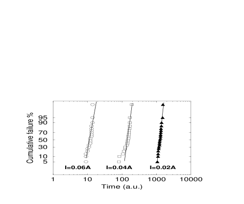
Figure 6: Distribution of TTFs obtained from $20$ simulations of failure at different stressing currents. The network sizes and the parameter values are the same of Fig. 5. Lines show the fit with a log-normal distribution.

It is interesting to consider the distribution of the times to failure (TTF) of a set of identical samples in the same stress conditions. Therefore we report in Figure 6 the distribution of the TTF obtained by simulations, at increasing values of the stressing current (going from the right to the left). All the parameters are the same of that used for Fig. 5. For each current value, 20 realizations have been considered. Precisely, in the figure the cumulative failure percentage is reported as a function of the logarithm of the TTF and a transformation has been applied to the ordinate axis in such a manner that a log-normal distribution would be a straight line. From the figure we can conclude that the distribution of the simulated TTF is log-normal (within errors) and that the shape factor (the log-normal standard deviation) is independent of the applied current. These conclusions well agree with the experiments [1, 2, 3]. As a result of the competition between the electromigration and the backflow of mass determined by stress gradients, the failure can occur or not depending on the length of the line. As a consequence, it is possible to consider this geometrical effects on the value of the MTF. Figure 7 shows the simulated MTF as function of the length to width ratio of the network (with fixed width). We remark that the MTF diverges for small lengths, according with the experimental results [2]. Experiments also show that for a line of given length it exists a critical value of the current density below which there is no electromigration. Moreover, this breakdown value is inversely proportional to the length [1, 2, 3]. Our simulations well reproduce also this behavior as shown in Fig. 8, where the breakdown current is reported as a function of the width to length ratio (again at width fixed).

Figure 7: Median time to failure as a function of the length to width ratio at fixed width. The network width and the parameter values are the same of Fig. 5. Points are the results of average over $20$ failure simulations.

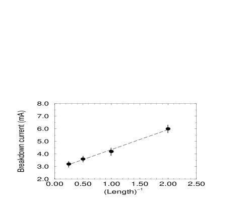
Figure 8: Breakdown current as a function of the width to length ratio at fixed width. The network width and the parameter values are the same of Fig. 5. The curve is a linear fit to data.

4 Conclusions

We have developed a Monte Carlo approach to electrical breakdown phenomena, with particular attention on its applications to the study of electromigration in metallic lines. Simulations are performed on a RRN whose configuration is evolving because of two competing percolations driven by an external current. The results of the simulations well agree with the experimental findings concerning several features of the electromigration phenomenon, including compositional and geometrical effects. The flexibility of the approach allows wide possibilities of further extentions of the model. Future goals are the extraction of information about precursor effects of the electical breakdown phenomena.

References

- [1] M. Ohring Reliability and Failure of Electronic Materials and Devices, Academic Press, San Diego (1998).
- [2] A. Scorzoni, B. Neri, C. Caprile, F. Fantini, Material Science Reports, 7, 143 (1991).
- [3] F. Fantini, J. R. Lloyd, I. De Munari, and A. Scorzoni, Microelectronic Engineering, 40, 207 (1998).
- [4] I. A. Blech, J. Appl. Phys. 47, 1203 (1976).
- [5] D. Stauffer and A. Aharony, Introduction to Percolation Theory, (Taylor and Francis, 1992).
- [6] C. Pennetta, L. Reggiani and G. Trefán, Phys. Rev. Lett. 84, 5006, (2000).
- [7] C. Pennetta, L. Reggiani, G. Trefán, F. Fantini, A. Scorzoni and I. De Munari J. Phys. D: Appl. Phys. 34, 1421 (2001).
- [8] J. R. Black, in Proc. of 5th IEEE International Reliability Physics Symposium p.148, (1967).
- [9] M. Shatzkes and J. R. Lloyd, J. Appl. Phys. 59, 3890 (1986).
- [10] J.J. Clement and J. R. Lloyd, J. Appl. Phys. 71, 1729 (1992).
- [11] M. Tammaro and B. Setlik, J. Appl. Phys., 85, 7127 (1999).