Semi-Flexible Polymer in a Uniform Force Field in Two Dimensions

Abstract

The conformational properties of a semi-flexible polymer chain, anchored at one end in a uniform force field, are studied in a simple two-dimensional model. Recursion relations are derived for the partition function and then iterated numerically. We calculate the angular fluctuations of the polymer about the direction of the force field and the average polymer configuration as functions of the bending rigidity, chain length, chain orientation at the anchoring point, and field strength.

I Introduction

The influence of external forces on the conformational properties of polymers has been studied extensively in recent years. Polymers stretched by attached magnetic beads smit92 , by laser tweezers smit96 ; wang97 , and by optical fibers cluz96 and polymers in flow fields perk95 ; lars97 ; smit99 ; lado00 have received much of the attention bust00 . The study of polymer deformation in elongational flow goes back to the prediction of a coil-stretch transition genn74 ; genn79 and early birefringence and light scattering experiments full80 ; kell85 . Experimental techniques perk95 ; perk94 ; kaes94 ; perk97 which allow direct visualization of polymer conformations in simple flows have given this field a new perspective. Here the main idea is to use fluorescently labelled DNA molecules, which are long enough so that their conformations can be resolved in an optical microscope.

In contrast to typical synthetic polymers, DNA chains are semi-flexible, with a persistence length of about 80 nm. For contour lengths of a few microns or more these chains behave as flexible polymers, in the absence of external forces. In the case of highly stretched DNA chains the bending rigidity has been shown to play an important role bust94 ; mark95 .

The force-extension curve of a semi-flexible polymer pulled at both ends is derived in Ref. mark95 . Predicting the deformation of a polymer in a flow field is considerably more complicated for two reasons. First, there is a direct hydrodynamic interaction between different polymer segments cifr99 ; rzeh99 ; rzeh00 . Second, even if the conformation-dependent, fluctuating drag on each bead is approximated by a friction term proportional to the local flow velocity (“free-draining” approximation), the force on each bead depends on the positions of all other beads. Thus, most theoretical studies have relied on computer simulations lars97 ; cifr99 ; rzeh99 ; rzeh00 ; lars99 and/or consider flexible chains cifr99 ; broc94 ; broc95 ; gg:gomp95f ; wink97 .

In this paper we study the conformational properties of a semi-flexible chain, anchored at one end, in two dimensions in a constant force field. In our model the polymer partition function is determined by simple recursion relations, which are easily iterated numerically. Very little computing time is required, and there is no statistical error in the results, but some other approximations, such as the Villain approximation vill75 , are involved, as will become clear.

The two-dimensional model of a semi-flexible polymer is described in Section II. Recursion relations for the partition function are derived in Section III. In Section IV we calculate the angular fluctuations of the polymer segments about the direction of the applied force, and in Section V the longitudinal extension due to the force. In Section VI we vary the angle between the polymer and the force field at the anchoring point and see how this affects the mean polymer configuration. Finally, in Section VII the case of a polymer pulled at its ends is briefly considered.

II The model

In the wormlike chain model of a semi-flexible polymer, the Hamiltonian is given by doi86

$${\cal H}_{0}=\frac{\kappa}{2}\int_{0}^{L}ds\;(\partial_{s}{\bf t})^{2}\;,$$ (1)

where ${\bf t}$ is a unit tangent vector and $s$ is the arc length. We consider a discrete version of this model in two spatial dimensions, with Hamiltonian

$${\cal H}_{0}=J\sum_{i=1}^{N}(\theta_{i}-\theta_{i-1})^{2}\;.$$ (2)

The polymer chain consists of $N+1$ line segments of fixed unit length. The $i$th segment forms an angle $\theta_{i}$ with the $x$ axis. One end of the polymer is anchored at the origin, and the orientation angle $\theta_{0}$ of the first segment is also assumed to be fixed.

To include a uniform force field $F_{0}$ in the $x$ direction, we add the terms

$${\cal H}_{1}=-F_{0}\sum_{i=1}^{N}x_{i}=-F_{0}\sum_{i=1}^{N}\sum_{j=1}^{i}\cos\theta_{j}=-F_{0}\sum_{i=1}^{N}(N+1-i)\cos\theta_{i}$$ (3)

to the Hamiltonian. The external field could be an electric, gravitational, or uniform flow field. The partition function corresponding to Eqs. (2) and (3) is given by

$$Z_{N}=\int_{-\infty}^{\infty}d\theta_{1}...\int_{-\infty}^{\infty}d\theta_{N}\;\exp\left\{-\sum_{i=1}^{N}\left[K(\theta_{i}-\theta_{i-1})^{2}+\hat{L}(N+1-i)\cos\theta_{i}\right]\right\}\;,$$ (4)

where $K=J/kT$ and $\hat{L}=F_{0}/kT$.

A nice feature of this model is that it can be solved exactly in the absence of an external field, i.e. for $\hat{L}=0$. The mean square end-to-end distance is given by

$$\langle R_{N}^{2}\rangle=N+1+\frac{2}{e^{1/\xi}-1}\left[N-\frac{1-e^{-N/\xi}}{e^{1/\xi}-1}\right]$$ (5)

with the persistence length $\xi=4K$. For $N\gg\xi\gg 1$, $\langle R_{N}^{2}\rangle\simeq(1+2\xi)N$, corresponding to an ideal flexible chain with Kuhn length $1+2\xi$. In the limit $N\ll\xi$ with $\xi\gg 1$, $\langle R_{N}^{2}\rangle\simeq(N+1)^{2}$, corresponding to a rigid rod.

To obtain a more tractable model, we make the Villain approximation vill75

$$\exp\left[\hat{L}\cos\theta\right]\to\sum_{m=-\infty}^{\infty}\exp\left[-L(\theta-2\pi m)^{2}\right]\;,$$ (6)

in Eq. (4). It was originally introduced in studies of the two-dimensional $x-y$ model and the roughening transition, where the Hamiltonians have a similar form. The approximation preserves the periodicity of the cosine function but leads to more manageable Gaussian integrals. An irrelevant normalization factor on the right-hand-side has been omitted. The constant $L$ may be determined by expanding both sides of Eq. (6) in Fourier series and equating the lowest two Fourier coefficients. This yields vill75

$$L=\left[4\ln\frac{I_{0}(\hat{L})}{I_{1}(\hat{L})}\right]^{-1}\;,$$ (7)

where $I_{0},I_{1}$ are modified Bessel functions.

Replacing $\sum_{m=-\infty}^{\infty}$ in Eq. (6) by $\sum_{m=-m_{\rm max}}^{m_{\rm max}}$ defines a further approximation, which may be systematically improved by increasing $m_{\rm max}$. In the finite $m_{\rm max}$ approximation, configurations with up to $m_{\rm max}$ loops about the origin receive the same statistical weight as for $m_{\rm max}=\infty$, but the statistical weight of configurations with more than $m_{\rm max}$ loops is underestimated.

III Recursion relations

As a first approximation we neglect all but the $m=0$ term in Eq. (6), replacing $e^{\hat{L}\cos\theta}$ by $e^{-L\theta^{2}}$. This is a good approximation for sufficiently large $K$ and/or $L$. The corresponding partition function is

$$Z_{N}^{0}(h_{1}, \dots ,h_{N})=\int_{-\infty}^{\infty}d\theta_{1}...\int_{-\infty}^{\infty}d\theta_{N}$$ (8)

$$\times \exp\left\{\sum_{i=1}^{N}\left[-K(\theta_{i}-\theta_{i-1})^{2}-L_{i}\theta_{i}^{2}+h_{i}\theta_{i}\right]\right\}\;,$$

where

$$L_{i}=(N+1-i)L\;,$$ (9)

as follows from Eq. (4). The $h_{i}$ are auxiliary variables that will be used in calculating thermal averages.

The partition function (8) may be evaluated by straightforward integration over $\theta_{1},\theta_{2},\dots$. The first $k-1$ integrations contribute

$$Q_{k}^{0}(\theta_{k}) = \int_{-\infty}^{\infty}d\theta_{1}...\int_{-\infty}^{\infty}d\theta_{k-1}\;\exp\left\{\sum_{i=1}^{k}\left[-K(\theta_{i}-\theta_{i-1})^{2}-L_{i}\theta_{i}^{2}+h_{i}\theta_{i}\right]\right\}\;,$$ (10)

$$= q_{k}\exp\left[-\gamma_{k}\theta_{k}^{2}+2\beta_{k}\theta_{k}\right]\;,$$

where $q_{k}$ is a constant, independent of $\theta_{k}$. Equation (10) and the recursive property

$$Q_{k}^{0}(\theta_{k})=\int_{-\infty}^{\infty}d\theta_{k-1}\;\exp\left[-K(\theta_{k}-\theta_{k-1})^{2}-L_{k}\theta_{k}^{2}+h_{k}\theta_{k}\right]Q_{k-1}^{0}(\theta_{k-1})$$ (11)

imply

$$q_{k}=\left(\frac{\pi}{\gamma_{k-1}+K}\right)^{1/2}\exp\left[\frac{\beta_{k-1}^{2}}{\gamma_{k-1}+K}\right]q_{k-1}\;,$$ (12)

where

$$\gamma_{1} = K+L_{1}\;,$$ (13)

$$\gamma_{k} = \frac{K\gamma_{k-1}}{\gamma_{k-1}+K}+L_{k}\;,\qquad k=2,\dots,N\;,$$ (14)

$$\beta_{1} = K\theta_{0}+\frac{1}{2}h_{1}\;,$$ (15)

$$\beta_{k} = \frac{K\beta_{k-1}}{\gamma_{k-1}+K}+\frac{1}{2}h_{k}\;,\qquad k=2,\dots,N\;.$$ (16)

Iterating Eq. (12) to obtain $q_{N}$ and using $Z_{N}^{0}=\int d\theta_{N}Q_{N}^{0}(\theta_{N})=$
$=(\pi/\gamma_{N})^{1/2}\exp\left[\beta_{N}^{2}/\gamma_{N}\right]q_{N}$, as follows from Eqs. (8) and (10), we obtain

$$Z_{N}^{0} = \left[\frac{\pi}{\gamma_{N}}\;\frac{\pi}{\gamma_{N-1}+K}\dots\frac{\pi}{\gamma_{1}+K}\right]^{1/2}$$ (17)

$$\times \exp\left[\frac{\beta_{N}^{2}}{\gamma_{N}}+\frac{\beta_{N-1}^{2}}{\gamma_{N-1}+K}+\dots+\frac{\beta_{1}^{2}}{\gamma_{1}+K}\right]\;.$$

The partition function (17) is completely determined by the recursion relations (13)-(16) and the $L_{i}$ defined in Eq. (9).

IV Angular fluctuations

We now derive the angular fluctuations $\langle\theta_{i}^{2}\rangle$ of the polymer chain in a constant force field from the partition function $Z_{N}^{0}$ of Eqs. (8) and (9). In this section we set the initial angle $\theta_{0}$ and all of the auxiliary variables $h_{i}$ equal to zero. In this case

$$K\langle\theta_{i}^{2}\rangle=f_{i}(L/K,N)$$ (18)

only depends on $K$ and $L$ in the combination $L/K$. This follows from rescaling the angles $\theta_{i}$ in the partition function (8). A second consequence is that the $\beta_{k}$ in Eqs. (15)-(17) all vanish.

Using the definition (9) of $L_{i}$, we write the recursion relation (14) for $\gamma_{k}$ in the form

$$\gamma_{k}=K+L(N+1-k)-\frac{K^{2}}{K+\gamma_{k-1}}\;.$$ (19)

According to Eqs. (9), (17), and (19) the angular fluctuations $\langle\theta_{i}^{2}\rangle=-\partial\ln Z_{N}^{0}/\partial L_{i}$ satisfy

$$\langle\theta_{k}^{2}\rangle = \frac{1}{2(\gamma_{k}+K)}+\left(\frac{K}{\gamma_{k}+K}\right)^{2}\langle\theta_{k+1}^{2}\rangle\;,\quad k=1,\dots,N-1\;,$$ (20)

$$\langle\theta_{N}^{2}\rangle = \frac{1}{2\gamma_{N}}\;.$$ (21)

We have calculated $\langle\theta_{i}^{2}\rangle$ by numerical iteration of Eqs. (13), (19), (20), and (21). The results for $L/K=0.1$ and $N=100$, $500$, $1000$ are shown in Fig. 1. For these three values of $N$ the results for $\langle\theta_{N}^{2}\rangle$ in Fig. 1 are practically indistinguishable. The same is true of $\langle\theta_{N-1}^{2}\rangle$, $\langle\theta_{N-2}^{2}\rangle$, etc. The values $N=100$, $500$, and $1000$ are large enough so that the angular fluctuations at the free end of the chain are independent of the chain length.

We now examine the $N$-dependence of the fluctuations. In Fig. 2 the quantity $K\langle\theta_{N}^{2}\rangle$ is plotted as a function of $N$ for five different values of $L/K$. There is an obvious crossover from $N$-dependent to $N$-independent behavior as $N$ increases. We denote the approximate value of $N$ at the crossover by $N_{\rm min}$. According to Eq. (18), $N_{\rm min}$ only depends on $K$ and $L$ in the combination $L/K$. Fig. 3 shows $N_{\rm min}$ as a function of $L/K$. The data are in excellent agreement with

$$N_{\rm min}\sim(L/K)^{-1/3},\quad L/K\ll 1\;.$$ (22)

The power law (22) follows from the following argument: For $L/K\ll 1$ the recursion relation (19) implies

$$\gamma_{k}=\frac{K}{k}\left[1+kA_{k}\frac{L}{K}+O\left((L/K)^{2}\right)\right]$$ (23)

where $A_{k}$ satisfies the recursion relation

$$A_{k}=\left(\frac{k-1}{k}\right)^{2}A_{k-1}+(N+1-k)$$ (24)

with $A_{1}=N$. Since the factor multiplying $A_{k-1}$ in Eq. (24) approaches unity as $k$ increases, $A_{N}\sim N^{2}$ for $N\gg 1$. For fixed $L/K\ll 1$ and $N$ small, the first term in $\gamma_{N}$, as given by Eq. (23), is clearly the dominant term, and $\gamma_{N}\simeq K/N$. However, the second term becomes increasingly important as $N$ increases. It is reasonable to assume that a crossover to a different $L/K$ dependence occurs when the second term in $\gamma_{N}$, as given by Eq. (23), becomes comparable with the first, i.e. $NA_{N}\sim N^{3}\sim K/L$ for $N\sim N_{\rm min}$. This leads to Eq. (22) and the prediction $\gamma_{N}\sim\gamma_{N_{\rm min}}\sim K(L/K)^{1/3}$ for $L/K\ll 1$, $N\gg N_{\rm min}$.

In the complementary regime $L/K\gg 1$ the recursion relation (19) implies

$$\gamma_{N}=K\left[\frac{L}{K}+1-\frac{K}{2L}+O\left((K/L)^{2}\right)\right]$$ (25)

for arbitrary $N$. Since this result is entirely independent of $N$, the large $N$ behavior has its onset at

$$N_{\rm min}\sim 1,\quad L/K\gg 1\;.$$ (26)

We now derive exact analytic expressions for the fluctuations $\langle\theta_{N}^{2}\rangle$, $\langle\theta_{N-1}^{2}\rangle,\dots$ at the end of an infinitely long chain. Reverse iteration of Eq. (19), beginning with $\gamma_{N}$, leads to the continued fraction

$$\gamma_{N}=K+L-\frac{K^{2}}{2K+2L\;-\ }\ \frac{K^{2}}{2K+3L\;-\ }\ \frac{K^{2}}{2K+4L\;-\ }\ \dots\ \frac{K^{2}}{2K+NL}\;.$$ (27)

In the limit $N\to\infty$ the continued fraction may be evaluated with the help of Eq. (9.1.73) in Ref. abra70 , yielding

$$\gamma_{\infty}=K\left[\frac{J_{\nu}(\nu)}{J_{\nu}^{\prime}(\nu)}-1\right]^{-1}\;,\quad\nu=\frac{2K}{L}\;.$$ (28)

Here $J_{\mu}(z)$ is the standard Bessel function, and $J_{\mu}^{\prime}(z)$ is its derivative with respect to $z$. From Eq. (9.3.23) in Ref. abra70 and Eq. (27), we obtain

$$\gamma_{\infty}\simeq K\left\{\begin{array}[]{l}\displaystyle{3^{1/3}\frac{\Gamma(2/3)}{\Gamma(1/3)}\left(\frac{L}{K}\right)^{1/3}\;,}\\ \\ \displaystyle{\frac{L}{K}+1-\frac{K}{2L},}\end{array}\right.\begin{array}[]{l}\displaystyle{\frac{L}{K}\ll 1}\;,\\ \\ \displaystyle{\frac{L}{K}\gg 1}\;.\end{array}$$ (29)

These limiting forms are consistent with the expressions for $\gamma_{\infty}\sim\gamma_{N_{\rm min}}$ for small and large $L/K$ given in Eq. (25) and the paragraph which preceeds it.

¿From the result (28) for $\langle\theta_{N}^{2}\rangle=\left(2\gamma_{N}\right)^{-1}$ in the large-$N$ limit, it is straightforward to calculate $\langle\theta_{N-1}^{2}\rangle$, $\langle\theta_{N-2}^{2}\rangle,\dots$ using Eqs. (19)-(21).

In Fig. 4, $K\langle\theta_{N}^{2}\rangle=K/(2\gamma_{N})$ is plotted as a function of $L/K$ for $N=10$, $100$, $1000$, and compared with the analytic prediction (28) for $N\to\infty$.

As stated in Section III, the $m_{\rm max}=0$ approximation is accurate for sufficiently large $K$ and/or $L$. One can use the results of this section to determine the domain of validity more precisely. The approximation, i.e. replacing $\cos\theta$ by $1-\frac{1}{2}\theta^{2}$, should be quite reliable if, say, $\langle\theta_{N}^{2}\rangle=\left(2\gamma_{N}\right)^{-1}<(\pi/4)^{2}$ or $\gamma_{N}>8/\pi^{2}\simeq 1$. Computing $\gamma_{N}$ by numerical iteration, one can readily check whether this inequality is satisfied for particular values of $K$, $L$, and $N$. According to Eqs. (23), (29), and (25), the inequality $\gamma_{N}>1$ corresponds to $K>N$ for $L/K\ll 1$ and $N\ll N_{\rm min}$, to $K(L/K)^{1/3}>1.4$ for $L/K\ll 1$ and $N\gg N_{\rm min}$, and to $L>1$ for $L/K\gg 1$ and arbitrary $N$.

V Longitudinal stretching

For a polymer in a constant force field, one of the main quantities of interest is the average extension in the flow direction. According to a prediction of Marko and Siggia mark95 ,

$$\frac{\langle x_{N}\rangle}{N}\simeq 1-C_{0}(LKN)^{-1/2}\;,$$ (30)

with $C_{0}=1$. This result was derived by approximating the restoring force at position $s$ along the chain with the thermodynamic result for a polymer of length $s$ pulled at its ends. Note, however, that a polymer in a flow field fluctuates most strongly at the free end and not at all at the anchored end, quite unlike a polymer pulled at its ends. The derivation also assumes a boundary condition $\langle\cos\theta_{N}\rangle\sim LK^{2}\ll 1$ at the end of the chain, at odds with the exact result $\langle\theta_{N}^{2}\rangle\sim(LK^{2})^{-1/3}$ in Eqs. (21) and (29) for large $K$ and $N$, where our discrete model is equivalent to the continuum model of Ref. mark95 . One advantage of our approach is that it avoids these assumptions and yields numerically exact results for the model with partition function (8).

We have checked Eq. (30) for our model, using the relations

$$\langle x_{N}\rangle = \sum_{j=0}^{N}\langle\cos\theta_{j}\rangle=\frac{1}{2}\sum_{j=0}^{N}\langle e^{i\theta_{j}}+e^{-i\theta_{j}}\rangle\;,$$ (31)

$$\langle e^{\pm i\theta_{j}}\rangle = \frac{Z_{N}^{0}(0,\dots,h_{j}=\pm i,0,\dots)}{Z_{N}^{0}(0,\dots,0)}\;.$$ (32)

Here the numerator on the right side of Eq. (32) is the partition function of Eqs. (8) and (17) with all of the auxiliary fields set equal to zero except that $h_{j}=i$. In the denominator all of the auxiliary fields, including $h_{j}$, vanish.

Calculating these partition functions recursively using Eqs. (13), (14), and (17), with the $L_{i}$ defined by Eq. (9), we obtained the results for the extension shown in Fig. 5. The data for sufficiently large $K$ do indeed confirm Eq. (30). For our model $C_{0}\simeq 0.23$.

It is instructive to compare the chain length $N$ with $N_{min}$ in the regime where Eq. (30) applies. For $K=1000$ and $N=10\thinspace 000$ (filled circular points in Fig. 5) the six-decade interval $10^{0}<LKN<10^{6}$ corresponds to $10^{-10}<L/K<10^{-4}$, or (see Eq. (22) and Fig. 3) to $20\thinspace 000>N_{min}>200$. Thus, the inequality $N\gg N_{min}$ only holds for the last three decades of $LKN$.

There are deviations from the straight line in Fig. 5 for smaller $K$ and larger $L$. For $L\gg K$, the recursion relation (19) implies

$$\gamma_{k}\simeq(N+1-k)L\;,$$ (33)

and

$$\langle x_{N}\rangle=\sum_{i=0}^{N}\langle\cos\theta_{i}\rangle\simeq N-\frac{1}{2}\sum_{i=0}^{N}\langle\theta_{i}^{2}\rangle\simeq N-\frac{1}{4}\sum_{i=0}^{N}\frac{1}{\gamma_{i}}\;.$$ (34)

The sum over the chain segments is easily carried out and yields

$$\langle x_{N}\rangle\simeq N-\frac{\ln N}{4L}.$$ (35)

In Fig. 6 numerical data for several bending rigidities, chain lengths and force fields are compared with this result. The agreement is excellent. Thus, for a sufficiently strong force field or a sufficiently small bending rigidity, the chain extension varies as $L^{-1}$, just as for flexible chains with arbitrary $L$.

VI Mean polymer configuration for $\theta_{0}\neq 0$

In this section we consider polymer conformations with the first segment fixed at a non-zero angle $\theta_{0}$ with respect to the direction of the force field. We make the Villain approximation and restrict the sum in Eq. (6) to $m=-1,0,1$. In the corresponding polymer partition function there is a separate sum over $m$ for each polymer segment. For a sufficiently stiff polymer and/or a sufficiently strong force field, the conformations of the chain are dominated by the same potential minimum. In this case the separate sums may be replaced by a single sum, leading to the simpler partition function

$$\tilde{Z}_{N}(\tilde{h}_{1}, \dots ,\tilde{h}_{N})=\sum_{m=-1}^{1}\int_{-\infty}^{\infty}d\theta_{1}...\int_{-\infty}^{\infty}d\theta_{N}$$ (36)

$$\times \exp\left\{\sum_{i=1}^{N}\left[-K(\theta_{i}-\theta_{i-1})^{2}-L_{i}(\theta_{i}-2\pi m)^{2}+\tilde{h}_{i}\theta_{i}\right]\right\}\;.$$

Here we have again introduced a set of auxiliary variables $\tilde{h}_{i}$, to be used in constructing thermal averages.

Expanding $(\theta_{i}-2\pi m)^{2}$ in powers of $\theta_{i}$, one sees that the partition function (36) can be expressed as

$$\tilde{Z}_{N}(\tilde{h}_{1},\dots,\tilde{h}_{N})=\sum_{m=-1}^{1}e^{-4\pi^{2}m^{2}(L_{1}+\dots+L_{N})}Z_{N}^{0}(\tilde{h}_{1}+4\pi mL_{1},\dots,\tilde{h}_{N}+4\pi mL_{N})$$ (37)

in terms of the $m=0$ partition function $Z_{N}^{0}(h_{1},\dots,h_{N})$ defined in Eq. (17). Since we know how to calculate $Z_{N}^{0}$ numerically with the recursion relations of Section III, we can also calculate $\tilde{Z}_{N}$ via Eq. (37). Using Eqs. (9), (13)-(17), (37), and the relations

$$\langle x_{k}\rangle = \sum_{j=0}^{k}\langle\cos\theta_{j}\rangle=\frac{1}{2}\sum_{j=0}^{k}\langle e^{i\theta_{j}}+e^{-i\theta_{j}}\rangle\;,$$ (38)

$$\langle y_{k}\rangle = \sum_{j=0}^{k}\langle\sin\theta_{j}\rangle=\frac{1}{2i}\sum_{j=0}^{k}\langle e^{i\theta_{j}}-e^{-i\theta_{j}}\rangle\;,$$ (39)

$$\langle e^{\pm i\theta_{j}}\rangle = \frac{\tilde{Z}_{N}(0,\dots,\tilde{h}_{j}=\pm i,0,\dots)}{\tilde{Z}_{N}(0,\dots,0)}\;,$$ (40)

we have evaluated the average position of the $j$th segment of the polymer chain for fixed $\theta_{0}$.

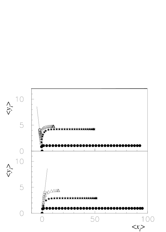
Figure 7: Average positions $\langle x_{i}\rangle,\langle y_{i}\rangle$ of a chain of length $N=100$ with $K=1$, $\theta_{0}=\pi/3$ (lower panel), and $\theta_{0}=2\pi/3$ (upper panel), with $L=10^{-5}$ $(\circ)$, $L=10^{-4}$ $(\triangle)$, $L=10^{-3}$ $(\star)$, $L=10^{-1}$ $(\bullet)$. The straight line indicates the tilt angle $\theta_{0}$.

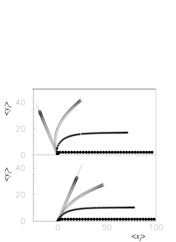
Figure 8: Average positions $\langle x_{i}\rangle,\langle y_{i}\rangle$ of a chain of length $N=100$ with $K=10$, $\theta_{0}=\pi/3$ (lower panel), and $\theta_{0}=2\pi/3$ (upper panel), with $L=10^{-5}$ $(\circ)$, $L=10^{-4}$ $(\triangle)$, $L=10^{-3}$ $(\star)$, $L=10^{-1}$ $(\bullet)$. The straight line indicates the tilt angle $\theta_{0}$.

Figs. 7-12 show how the average position depends on the tilt angle $\theta_{0}$, field strength $L$, and bending rigidity $K$. In all of these figures $N=100$.

Figs. 7 and 8 show the average polymer configuration in the $x,y$ plane. As the field strength increases, the polymer is bent towards the field direction and is stretched longitudinally. The elongation is more pronounced for smaller bending rigidities.

In Fig. 9 the transverse extension of the polymer as a function of the tilt angle is shown in more detail. The curves are sinusoidal for small field strengths $L$ but for larger $L$ bend abruptly near $\theta_{0}=\pm\pi$, due to the instability of a polymer directed against the force field. Since our model includes fluctuations, the polymer ”tunnels” between the two equivalent free-energy minima, and there is no spontaneous symmetry breaking at $\theta_{0}=\pi$.

Fig. 10 shows the tranverse extension as a function of the field strength for three different $\theta_{0}$. For $K=10$, $N=100$, and $L<10^{-5}$, the effect of the force field is negligible. For stronger force fields, there seems to be a regime where $\langle y_{N}\rangle\sim L^{-2/5}$.

The contour length $C_{l}$ of the average configuration (see Figs. 7 and 8) is shown in Fig. 11. Again, the effect of the force field is negligible for $K=10$, $N=100$, and $L<10^{-5}$ . Varying the tilt angle only affects the contour length near the onset of the deformation due to the force field.

Finally, we have considered the angle $\delta$ between a line through the end-points of the chain and the direction of the force field. A weak force field deforms the polymer only slightly, and $\delta$ varies linearly with the tilt angle $\theta_{0}$. For a strong force field, on the other hand, $\delta$ varies abruptly as $\theta_{0}$ approaches $\pi$, due to the instability mentioned above. The behavior of $\delta$ as a function of $L$ in Fig. 12 is qualitatively similar to that of $\langle y_{N}\rangle$ in Fig. 10.

VII Polymer pulled at its ends

Thus far we have considered an external force field that acts on each monomer of the semi-flexible polymer. With only minor modifications the case of a constant force applied at the ends of the polymer can also be studied. Anchoring one end at the origin at a fixed angle $\theta_{0}$, we apply a constant force at the other end by replacing Eq. (3) with ${\cal H}_{1}=-F_{0}x_{N}=-F_{0}\sum_{j=1}^{N}\cos\theta_{j}$. In the Villain approximation (6) the partition function is again given by Eq. (8), but Eq. (9) is replaced by $L_{i}=L$. With this definition of the $L_{i}$ the partition function may be calculated recursively, as in Section III. For symmetric boundary conditions at the ends of the chain, i.e. $\theta_{0}$ and $\theta_{N}$ both fixed or both free to fluctuate, the calculation is also straightforward.

For fixed $\theta_{0}=0$ and fluctuating $\theta_{N}$, the angular fluctuations of the polymer segments are given by Eqs. (18), (20), and (21), with Eq. (19) replaced by

$$\gamma_{k}=K+L-\frac{K^{2}}{K+\gamma_{k-1}}\;.$$ (41)

In the long chain limit $\gamma_{N}$ approaches the fixed point

$$\gamma_{\infty}=\frac{L}{2}+\left[\left(\frac{L}{2}\right)^{2}+KL\right]^{1/2}$$ (42)

of Eq. (41).

For large $K$ and $N$ our discrete model is equivalent to the continuum model of Marko and Siggia mark95 . In this limit Eqs. (21) and (42) imply the same result $\langle\theta_{N}^{2}\rangle=(4KL)^{-1/2}$ for the angular fluctuations as in Ref. mark95 .

In Fig. 13, $K\langle\theta_{N}^{2}\rangle=K/(2\gamma_{N})$ is plotted as a function of $L/K$ for $N=10$, $100$, $1000$, and $10\thinspace 000$ and compared with the analytic prediction (42) for $N\to\infty$.

We have also calculated the mean configuration of a polymer pulled at its ends for fixed $\theta_{0}>0$ and fluctuating $\theta_{N}$. Fig. 14 shows the tranverse extension as a function of the force for three different $\theta_{0}$. For $K=10$, $N=100$, and $L<10^{-3}$, the effect of the force is negligible. For stronger forces there seems to be a regime where $\langle y_{N}\rangle\sim L^{-2/5}$. We found quite similar behavior for a polymer in a uniform force field, as shown in Fig. 10.

VIII Concluding remarks

For calculating the conformational properties of a semi-flexible chain in a uniform force field our recursive approach has several advantages: (i) It requires very little computing time, and (ii) it allows one to consider very long chains. For a clearly-defined model exact numerical results are obtained. Thus, (iii) there is no statistical error, and (iv) some of the approximations in earlier theoretical work are avoided. Finally, (v) the recursion relations furnish some analytical insight. We were able to obtain some exact results for the asymptotic behavior of long chains. While most previous studies have focused on the force-extension relation, we have also analyzed angular fluctuations.

A disadvantage of the approach is the limitation to two dimensions. However, many of the results probably apply, at least qualitatively, to chains in three spatial dimensions. Furthermore, the results are directly applicable to polymers confined to two dimensions, for example, DNA electrostatically bound to fluid lipid membranes maie99 .

The Villain approximation was used to obtain a tractable model. It preserves the periodicity in $\theta$ and is no more unrealistic than using a quadratic bending energy for arbitrary angles or ignoring excluded volume. We only presented results for the single-$m$ approximation with $m_{\rm max}\leq 1$, which underestimates the statistical weight of configurations with segments pointing in widely different directions but is accurate for sufficiently large $K$ and/or $L$.

The single-$m$ approximation can, of course, be improved at the cost of greater computing time. Retaining all the Villain sums leads to the partition function

$${\cal Z}_{N}(\tilde{h}_{1},\dots,\tilde{h}_{N}) = \sum_{m_{1}=-\infty}^{\infty}\dots\sum_{m_{N}=-\infty}^{\infty}e^{-4\pi^{2}m_{1}^{2}L_{1}}\dots e^{-4\pi^{2}m_{N}^{2}L_{N}}$$ (43)

$$\times\ Z_{N}^{0}(\tilde{h}_{1}+4\pi m_{1}L_{1},\dots,\tilde{h}_{N}+4\pi m_{N}L_{N})$$

instead of Eq. (37). Here $Z_{N}^{0}$ is the $m=0$ partition function in Eq. (17), which we know how to compute recursively. Usually one is interested in $K$ and $L$ for which the angular differences between adjacent segments are small, certainly less than $2\pi$. Then the sums on the right side of Eq. (43) may be restricted to the terms with $-1\leq m_{1}\leq 1$, $m_{1}-1\leq m_{2}\leq m_{1}+1$, etc. Computing ${\cal Z}_{N}$ with no further approximations requires $3^{N}$ evaluations of $Z_{N}^{0}$.

IX Acknowledgements

Helpful discussions with R. Winkler and U. Seifert are gratefully acknowledged. T.W.B. thanks the Institut für Festkörperforschung, Forschungszentrum Jülich for hospitality and the Alexander von Humboldt Stiftung for financial support.

Figure Captions

Figure 1: Average angular fluctuations $K\langle\theta_{i}^{2}\rangle$ for $L/K=0.1$ and $N=100$ $(\bullet)$, $N=500$ $(\star)$, $N=1000$ $(\ast)$.

Figure 2: Average angular fluctuations $K\langle\theta_{N}^{2}\rangle$ of the final chain segment as a function of $N$ for $L/K=10^{-5}$ $(\bullet)$, $L/K=10^{-4}$ $(\circ)$, $L/K=10^{-3}$ $(\triangle)$, $L/K=10^{-2}$ $(\star)$, $L/K=10^{-1}$ $(\ast)$. The straight line has slope 1.

Figure 3: $N_{\rm min}$ as a function of $L/K$ for $K=1$ $(\bullet)$, $K=10$ $(\circ)$, $K=100$ $(\triangle)$, $K=1000$ $(\star)$. The straight line has slope -1/3.

Figure 4: $K\langle\theta_{N}^{2}\rangle=K/(2\gamma_{N})$ for a polymer in a constant force field as a function of $L/K$ for $N=10$ ($\bullet$), $N=100$ ($\circ$), and $N=1000$ ($\triangle$), together with the exact result (28) for $N\to\infty$ ($\star$). The straight lines have slopes $-1/3$ and $-1$, respectively.

Figure 5: Average extension, $\langle x_{N}\rangle$ of the chain in the direction of the force field direction as a function of the field strength $L$, for $K=10$, $N=100$ ($\ast$); $K=10$, $N=1000$ ($\circ$); $K=10$, $N=10000$ ($\diamond$); $K=100$, $N=1000$ ($\triangle$); $K=100$, $N=10000$ ($\star$); $K=1000$, $N=10\thinspace 000$ ($\bullet$). The straight line has slope $-1/2$.

Figure 6: Average extension $\langle x_{N}\rangle$ of the chain in the direction of the force field as a function of the field strength $L$. The symbols correspond to the same parameters as in Fig. 5. The straight line has slope $-1$.

Figure 9: Average transverse extension $\langle y_{N}\rangle$ as a function of $\theta_{0}$ for $N=100$, $K=10$ and $L=10^{-9}$ $(\ast)$, $L=10^{-5}$ $(\star)$ , and $L=10^{-3}$ $(\triangle)$ , $L=10^{-2}$ $(\circ)$ , $L=10^{-1}$ $(\bullet)$.

Figure 10: Average transverse extension $\langle y_{N}\rangle$ as a function of $L$ for $N=100$, $K=10$, and $\theta_{0}=\pi/3$ $(\bullet)$, $\theta_{0}=2\pi/3$ $(\circ)$ , $\theta_{0}=17\pi/18$ $(\triangle)$.

Figure 11: Contour length $C_{l}$ of the average configuration as a function of $L$ for $N=100$, $K=10$, and $\theta_{0}=\pi/180$ $(\bullet)$, $\theta_{0}=\pi/3$ $(\circ)$, $\theta_{0}=2\pi/3$ $(\triangle)$.

Figure 12: Angle $\delta$ between a line through the end points of the chain and the direction of the force field as a function of $L$ for $N=100$, $K=10$, and $\theta_{0}=\pi/180$ $(\bullet)$, $\theta_{0}=\pi/3$ $(\circ)$, $\theta_{0}=2\pi/3$ $(\triangle)$.

Figure 13: $K\langle\theta_{N}^{2}\rangle=K/(2\gamma_{N})$ for a polymer pulled at the ends as a function of $L/K$ for $N=10$ ($\ast$), $N=100$ ($\triangle$), $N=1000$ ($\circ$), and $N=10\thinspace 000$ ($\bullet$), together with the exact result (42) for $N\to\infty$ ($\star$). The straight lines have slopes $-1/2$ and $-1$, respectively.

Figure 14: Average transverse extension $\langle y_{N}\rangle$ of a polymer pulled at its ends as a function of $L$ for $N=100$, $K=10$, and $\theta_{0}=\pi/3$ $(\bullet)$, $\theta_{0}=2\pi/3$ $(\circ)$, $\theta_{0}=17\pi/18$ $(\triangle)$.

Figure 1: Average angular fluctuations $K\langle\theta_{i}^{2}\rangle$ for $L/K=0.1$ and $N=100$ $(\bullet)$, $N=500$ $(\star)$, $N=1000$ $(\ast)$.

Figure 2: Average angular fluctuations $K\langle\theta_{N}^{2}\rangle$ of the final chain segment as a function of $N$ for $L/K=10^{-5}$ $(\bullet)$, $L/K=10^{-4}$ $(\circ)$, $L/K=10^{-3}$ $(\triangle)$, $L/K=10^{-2}$ $(\star)$, $L/K=10^{-1}$ $(\ast)$. The straight line has slope 1.

Figure 3: $N_{\rm min}$ as a function of $L/K$ for $K=1$ $(\bullet)$, $K=10$ $(\circ)$, $K=100$ $(\triangle)$, $K=1000$ $(\star)$. The straight line has slope -1/3.

Figure 4: $K\langle\theta_{N}^{2}\rangle=K/(2\gamma_{N})$ for a polymer in a constant force field as a function of $L/K$ for $N=10$ ($\bullet$), $N=100$ ($\circ$), and $N=1000$ ($\triangle$), together with the exact result (28) for $N\to\infty$ ($\star$). The straight lines have slopes $-1/3$ and $-1$, respectively.

Figure 5: Average extension, $\langle x_{N}\rangle$ of the chain in the direction of the force field direction as a function of the field strength $L$, for $K=10$, $N=100$ ($\ast$); $K=10$, $N=1000$ ($\circ$); $K=10$, $N=10000$ ($\diamond$); $K=100$, $N=1000$ ($\triangle$); $K=100$, $N=10000$ ($\star$); $K=1000$, $N=10\thinspace 000$ ($\bullet$). The straight line has slope $-1/2$.

Figure 6: Average extension $\langle x_{N}\rangle$ of the chain in the direction of the force field as a function of the field strength $L$. The symbols correspond to the same parameters as in Fig. 5. The straight line has slope $-1$.

Figure 7: Average positions $\langle x_{i}\rangle,\langle y_{i}\rangle$ of a chain of length $N=100$ with $K=1$, $\theta_{0}=\pi/3$ (lower panel), and $\theta_{0}=2\pi/3$ (upper panel), with $L=10^{-5}$ $(\circ)$, $L=10^{-4}$ $(\triangle)$, $L=10^{-3}$ $(\star)$, $L=10^{-1}$ $(\bullet)$. The straight line indicates the tilt angle $\theta_{0}$.

Figure 8: Average positions $\langle x_{i}\rangle,\langle y_{i}\rangle$ of a chain of length $N=100$ with $K=10$, $\theta_{0}=\pi/3$ (lower panel), and $\theta_{0}=2\pi/3$ (upper panel), with $L=10^{-5}$ $(\circ)$, $L=10^{-4}$ $(\triangle)$, $L=10^{-3}$ $(\star)$, $L=10^{-1}$ $(\bullet)$. The straight line indicates the tilt angle $\theta_{0}$.

Figure 9: Average transverse extension $\langle y_{N}\rangle$ as a function of $\theta_{0}$ for $N=100$, $K=10$ and $L=10^{-9}$ $(\ast)$, $L=10^{-5}$ $(\star)$ , and $L=10^{-3}$ $(\triangle)$ , $L=10^{-2}$ $(\circ)$ , $L=10^{-1}$ $(\bullet)$.

Figure 10: Average transverse extension $\langle y_{N}\rangle$ as a function of $L$ for $N=100$, $K=10$, and $\theta_{0}=\pi/3$ $(\bullet)$, $\theta_{0}=2\pi/3$ $(\circ)$ , $\theta_{0}=17\pi/18$ $(\triangle)$.

Figure 11: Contour length $C_{l}$ of the average configuration as a function of $L$ for $N=100$, $K=10$, and $\theta_{0}=\pi/180$ $(\bullet)$, $\theta_{0}=\pi/3$ $(\circ)$, $\theta_{0}=2\pi/3$ $(\triangle)$.

Figure 12: Angle $\delta$ between a line through the end points of the chain and the direction of the force field as a function of $L$ for $N=100$, $K=10$, and $\theta_{0}=\pi/180$ $(\bullet)$, $\theta_{0}=\pi/3$ $(\circ)$, $\theta_{0}=2\pi/3$ $(\triangle)$.

Figure 13: $K\langle\theta_{N}^{2}\rangle=K/(2\gamma_{N})$ for a polymer pulled at the ends as a function of $L/K$ for $N=10$ ($\ast$), $N=100$ ($\triangle$), $N=1000$ ($\circ$), and $N=10\thinspace 000$ ($\bullet$), together with the exact result (42) for $N\to\infty$ ($\star$). The straight lines have slopes $-1/2$ and $-1$, respectively.

Figure 14: Average transverse extension $\langle y_{N}\rangle$ of a polymer pulled at its ends as a function of $L$ for $N=100$, $K=10$, and $\theta_{0}=\pi/3$ $(\bullet)$, $\theta_{0}=2\pi/3$ $(\circ)$, $\theta_{0}=17\pi/18$ $(\triangle)$.

References

• (1) S. B. Smith, L. Finzi, and C. Bustamante, Science 258, 1122 (1992).
• (2) S. B. Smith, Y. J. Cui, and C. Bustamante, Science 271, 795 (1996).
• (3) M. D. Wang et al., Biophys. J. 72, 1335 (1997).
• (4) P. Cluzel et al., Science 271, 792 (1996).
• (5) T. T. Perkins, D. E. Smith, R. G. Larson, and S. Chu, Science 268, 83 (1995).
• (6) R. G. Larson, T. T. Perkins, D. E. Smith, and S. Chu, Phys. Rev. E 55, 1794 (1997).
• (7) D. E. Smith, H. P. Babcock, and S. Chu, Science 283, 1724 (1999).
• (8) B. Ladoux and P. S. Doyle, Europhys. Lett. 52, 511 (2000).
• (9) C. Bustamante, S. B. Smith, J. Liphardt, and D. Smith, Curr. Opin. Struct. Biol. 10, 279 (2000).
• (10) P.-G. de Gennes, J. Chem. Phys. 60, 5030 (1974).
• (11) P.-G. de Gennes, Scaling Concepts in Polymer Physics (Cornell University Press, Ithaca, 1979).
• (12) G. G. Fuller and L. G. Leal, Rheol. Acta 19, 580 (1980).
• (13) A. Keller and J. A. Odell, Colloid Polym. Sci. 263, 181 (1985).
• (14) T. T. Perkins, D. E. Smith, and S. Chu, Science 264, 819 (1994).
• (15) J. Käs, H. Strey, and E. Sackmann, Nature 368, 226 (1994).
• (16) T. T. Perkins, D. E. Smith, and S. Chu, Science 276, 2016 (1997).
• (17) C. Bustamante, J. F. Marko, E. D. Siggia, and S. Smith, Science 265, 1599 (1994).
• (18) J. F. Marko and E. D. Siggia, Macromolecules 28, 8759 (1995).
• (19) J. G. H. Cifre and J. G. de la Torre, J. Rheol. 43, 339 (1999).
• (20) R. Rzehak, D. Kienle, T. Kawakatsu, and W. Zimmermann, Europhys. Lett. 46, 821 (1999).
• (21) R. Rzehak, W. Kromen, T. Kawakatsu, and W. Zimmermann, Eur. Phys. J. E 2, 3 (2000).
• (22) R. G. Larson, H. Hu, D. E. Smith, and S. Chu, J. Rheol. 43, 267 (1999).
• (23) F. Brochard-Wyart, H. Hervet, and P. Pincus, Europhys. Lett. 26, 511 (1994).
• (24) F. Brochard-Wyart, Europhys. Lett. 30, 387 (1995).
• (25) D. M. Kroll and G. Gompper, J. Chem. Phys. 102, 9109 (1995).
• (26) R. G. Winkler and P. Reineker, J. Chem. Phys. 106, 2841 (1997).
• (27) J. Villain, J. Phys. (Paris) 36, 581 (1975).
• (28) M. Doi and S. F. Edwards, The Theory of Polymer Dynamics (Clarendon Press, Oxford, 1986).
• (29) Handbook of Mathematical Functions, edited by M. Abramowitz and I. A. Stegun (Dover Publications, New York, 1970).
• (30) B. Maier and J. O. Rädler, Phys. Rev. Lett. 82, 1911 (1999).