Dynamics of Magnetization Reversal in Models of Magnetic Nanoparticles and Ultrathin Films

Abstract

We discuss numerical and theoretical results for models of magnetization switching in nanoparticles and ultrathin films. The models and computational methods include kinetic Ising and classical Heisenberg models of highly anisotropic magnets which are simulated by dynamic Monte Carlo methods, and micromagnetics models of continuum-spin systems that are studied by finite-temperature Langevin simulations. The theoretical analysis builds on the fact that a magnetic particle or film that is magnetized in a direction antiparallel to the applied field is in a metastable state. Nucleation theory is therefore used to analyze magnetization reversal as the decay of this metastable phase to equilibrium. We present numerical results on magnetization reversal in models of nanoparticles and films, and on hysteresis in magnets driven by oscillating external fields.

1 Introduction

In recent years, the interest in nanostructured magnetic materials has soared for a variety of reasons. For one, it is only quite recently that it has become possible to synthesize and measure nanometer-sized magnetic particles in small, ordered arrays, often by techniques that involve modern, atomic-resolution microscopies, such as scanning-tunneling microscopy (STM), atomic force microscopy (AFM), or magnetic force microscopy (MFM) DORM92 ; CROM93 ; KENT93 ; KENT94 ; PAI97 . AFM and MFM pictures of an array of nanometer-sized iron pillars, fabricated by STM-assisted chemical vapor deposition GIDE96 , are shown in Fig. 1. The techniques are currently becoming precise enough to even allow investigation of individual nanoparticles. At the same time, computers have had a profound influence in two different ways. The need for ever higher data-recording densities has driven the size of particles used in recording media down into the nanometer range BERT94 ; CHOU94 ; NOVO99 , while the rapidly increasing power of computers has made it feasible to perform simulations of the dynamic properties of realistic model systems of sizes comparable to experimental ones RIKV97B ; NOWA01 ; BROW01 .

Figure 1: Array of nanoscopic iron pillars of dimensions approximately $40\times 40\times 200$ nm³, grown by STM-assisted chemical vapor deposition. (a) AFM image of the array of pillars, as grown on top of a $\umu$m-size Hall-effect magnetometer. (b) MFM image of the array after thermal randomization in near-zero applied field. The magnetic field from each pillar is imaged and seen to point along the major axis of the pillars, either up (white) or down (black). (c) MFM image of the array in an applied field of 200 G. Almost all the magnets are aligned with the field. Image data courtesy of D.D. Awschalom and J. Shi. (a) and (b) after GIDE96 A pdf version of this paper, which includes this figure, can be downloaded from http://www/csit.fsu.edu/$\sim{}$rikvold/abstracts/turkey.pdf

Modern magnetic recording technologies involve particles that are near the superparamagnetic limit. In this limit, the energy barrier separating the two energetically degenerate magnetic orientations is small enough that thermal fluctuations frequently lead to spontaneous switching of the orientation. As a result, the magnetic coercivity decreases with decreasing particle size for particles below the superparamagnetic size limit. The limit appears as a maximum in a curve showing switching field or coercivity versus particle size, such as in Fig. 2. Since the random magnetization reversals in particles below the superparamagnetic limit degrade recorded information, the engineering challenge has been to keep the energy barrier in the individual particles high enough to make spontaneous switching infrequent while keeping the material magnetically soft enough to facilitate recording. As the volumes of the magnetic particles have shrunk to reach recording densities on the order of 100 Gb/in² or more CHOU94 ; RUIG00 , materials with higher coercivities due to strong crystalline anisotropies have been employed WELLER2000 . In order to enhance engineering practices, it is essential to extend the physical understanding of the superparamagnetic limit past the theories of uniformly mangetized particles to include magnetization reversal dynamics that proceed through localized regions of reversed magnetization that subsequently spread throughout the magnetic element.

Figure 2: Effective switching field (analogous to coercivity) versus particle size for single-domain ferromagnetic barium ferrite particles ($\diamond$ with error bars, right vertical and top horizontal axes, experimental results) and for two-dimensional $L\times L$ Ising systems (data points connected by solid lines, left vertical and bottom horizontal axes). The barium ferrite data were digitized from Fig. 5 of CHAN93 . The Ising data are Monte Carlo simulations from RICH94 for waiting times $\tau$=100 Monte Carlo Steps per Site (MCSS) ($\circ$) and 1000 MCSS ($\times$) at $T$=0.8$T_{\rm c}$, where $T_{\rm c}$ is the exact Ising critical temperature. After RIKV94

The remainder of this article is organized as follows. In Sec. 2 we summarize some aspects of the theory of magnetization switching in anisotropic magnets, including effects of anisotropy (Sec. 2.1), nucleation theory (Sec. 2.2), and model systems (Sec. 2.3). In Sec. 3 we give some new results of finite-temperature micromagnetic simulations of magnetic nanoparticles. In Sec. 4 we discuss hysteresis in nanoparticles and ultrathin films, in particular the frequency dependence of hysteresis loops (Sec. 4.1) and a dynamic order-disorder phase transition (Sec. 4.2). A brief summary and conclusions are given in Sec. 5.

2 Theory of Magnetization Switching in Anisotropic Magnets

2.1 Effects of Magnetic Anisotropy

The most common description of magnetization switching is the mean-field, uniform-rotation theory of Néel NEEL49 and Brown BROW59 ; BROW63 . One assumes uniform rotation of all localized moments in the particle to avoid an energy barrier due to exchange interactions of strength $J$. The remaining barrier, $\Delta$, is caused by magnetic anisotropy – a combination of crystal-field and magnetostatic effects. The equilibrium thickness of a wall separating oppositely magnetized domains is $\ell_{\rm w}\propto\sqrt{J/\Delta}$. For particles smaller than $\ell_{\rm w}$ with small anisotropy, the uniform-rotation picture is reasonable. If the anisotropy is largely magnetostatic, the competition between exchange interactions and the demagnetizing field favors domains of opposite magnetization in particles larger than $\ell_{\rm w}$. The domains control switching through the field-driven motion of preexisting domain walls KOLE97B ; KOLE98C ; RIKV00B . However, if the anisotropy is largely crystalline, there exists a range of single-domain particle sizes that are larger than $\ell_{\rm w}$ but smaller than the size at which the particle becomes multidomain (often the case in ultrathin films HUG96 ).

In anisotropic nanomagnets the state of uniform magnetization opposite to the applied field constitutes a metastable phase. This nonequilibrium phase decays by thermally assisted nucleation and subsequent growth of localized regions, inside which the magnetization is parallel with the field RICH94 . These growing regions are referred to as droplets to distinguish them from equilibrium domains. This mechanism yields results very similar to recent experiments on single-domain nanoscale ferromagnets KOCH .

2.2 Application of Nucleation Theory to Magnetization Reversal

Here we present a short summary of homogeneous nucleation theory as it applies to uniaxial magnets. This theory covers situations in which the switching events are nucleated by thermal fluctuations, without the influence of defects. Further details are available in RIKV97B ; RICH94 ; RIKV94 ; RICH95C ; RICH96 ; TOMI92A ; RIKV94A .

The central problems in nucleation theory are to identify the fluctuations that lead to the decay of the metastable phase and to obtain their free-energy cost relative to the metastable phase. For anisotropic systems dominated by short-range interactions, these fluctuations are compact droplets of radius $R$. The free energy of the droplet has two competing terms: a positive surface term $\propto\sigma(T)R^{d-1}$ and a negative bulk term $\propto|H|R^{d}$ where $d$ is the spatial dimension, $\sigma(T)$ is the surface tension of the droplet wall, and $H$ is the applied magnetic field along the easy axis. Their competition yields a critical droplet radius, $R_{c}(H,T)\propto{\sigma(T)}/{|H|}$. Droplets with $R<R_{c}$ most likely decay, whereas droplets with $R>R_{c}$ most likely grow to complete the switching process. The free-energy cost of the critical droplet ($R=R_{c}$) is $\Delta F(H,T)\propto\sigma(T)^{d}/|H|^{d-1}$. Nucleation of critical droplets at nonzero temperature $T$ is a stochastic process with nucleation rate per unit volume given by an Arrhenius relation:

$$I(H,T)\propto|H|^{K}\exp\left[-{\beta\Delta F(H,T)}\right]\equiv|H|^{K}\exp\left[-{\beta\Xi(T)/|H|^{d-1}}\right]\;,$$ (1)

where $\beta=1/k_{\rm B}T$ ($k_{\rm B}$ is Boltzmann’s constant), $\Xi(T)$ is the $H$-independent part of $\Delta F$, and the prefactor exponent $K$ is known for many models from field-theoretical arguments RIKV94 ; LANG67 ; LANG69 ; GNW80 . The particles are of finite size $L$, and the dominant reversal mechanism depends on $H$, $T$, and $L$.

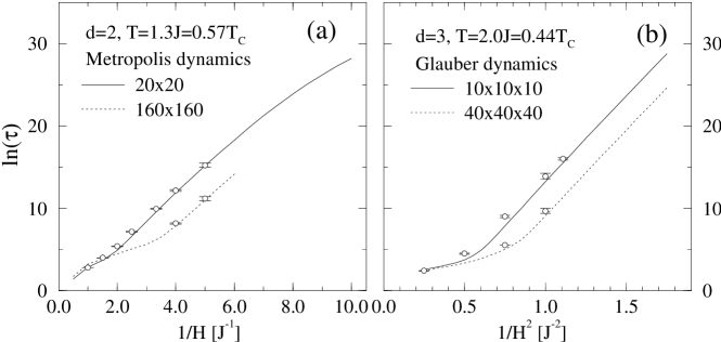
Figure 3: Lifetimes for two-dimensional $L^{2}$ Ising systems with $L=20$ and 160 at $T=0.57T_{c}$ (a), and three-dimensional $L^{3}$ Ising systems with $L=10$ and 40 at $T=0.44T_{c}$ (b). The data points are direct Monte Carlo simulation results, while the lines are extrapolations with the Projected Dynamics (PD) accelerated dynamics algorithm KOLE98B ; KOLE98A ; NOVO99B , based on the smallest system at the weakest field. The sharp changes in slope correspond to the DSp, with the deterministic regime to the left and the stochastic regime to the right. The ratio of the slopes of the curve in the single-droplet and multidroplet regimes is $(d+1)$, in agreement with (2) and (3). After KOLE98A

In the weakest applied fields, the particles are in the “Coexistence” (CE) regime, with the average metastable lifetime $\tau_{\rm CE}(H,T,L)\sim\exp\left[{2\beta\sigma(T)L^{d-1}}\right]$. (This result is nearly independent of the boundary conditions RICH96 .) The regime corresponds to $R_{\rm c}>L,$ and the associated $L$-dependent crossover field is called the Thermodynamic Spinodal (ThSp) RIKV94 ; TOMI92A ; RIKV94A . Estimating its value by assuming $R_{\rm c}(H,T,L)\approx L,$ one finds $H_{\rm ThSp}(T,L)\sim L^{-1}$. The $L$-dependence of $H_{\rm ThSp}$ is given by the dotted curve in Fig. 2.

For $|H|>H_{\rm ThSp}$ (but not too large), the lifetime is determined by the inverse of the total nucleation rate,

$$\tau_{\rm SD}(H,T,L)\approx\left(L^{d}I(H,T)\right)^{-1}\propto L^{-d}|H|^{K}\exp\left[{\beta\Xi(T)|H|^{d-1}}\right]\;,$$ (2)

which is inversely proportional to the particle volume, $L^{d}$ (see Fig. 3). The subscript SD stands for Single Droplet and indicates that in this regime the switching is normally completed by the first droplet to reach $R_{c}$. In both of the stochastic reversal regimes(CE and SD) the probability that switching has not taken place within a time $t$ after the field reversal, $P_{\rm not}(t)$, takes the form $P_{\rm not}(t)=\exp(-t/\tau)$.

A second crossover, called the Dynamic Spinodal (DSp) RIKV94 ; TOMI92A ; RIKV94A , is a consequence of the finite velocity, $v\approx\nu|H|$, of the surface of a growing supercritical droplet RIKV00B . A reasonable criterion to locate the DSp is that the average time between nucleation events, which is $\tau_{\rm SD}$, should equal the time it takes a droplet to grow to a size comparable to $L$. This yields the asymptotic relation $H_{\rm DSp}(T,L)\sim[\ln(L)]^{1/(d-1)}$. The $L$-dependence of $H_{\rm DSp}$ is given by the dashed curve in Fig. 2. For $|H|>H_{\rm DSp}$, the metastable phase decays through many droplets which nucleate and grow independently in different parts of the system. In this Multidroplet (MD) regime RIKV94 ; TOMI92A ; RIKV94A , the classical Kolmogorov-Johnson-Mehl-Avrami (KJMA) theory of metastable decay in large systems KOLM37 ; JOHN39 ; AVRAMI gives the lifetime

$$\tau_{\rm MD}(H,T)\propto\left[{I(H,T)(\nu|H|)^{d}}/{(d+1)\ln 2}\right]^{-{1}/{(d+1)}}\;,$$ (3)

independent of $L$ (see Fig. 3). In the MD regime $P_{\rm not}(t)\approx{\rm erfc}\left((t-\tau)/\Delta\right)$ RICH94 , where the width $\Delta$ of the switching-time distribution depends on $H$, $T$, and $L$.

[width=0.60]fig4_metaphasediag.eps

Figure 4: Metastable phase diagram for the two-dimensional Ising model at temperatures up to $T_{c}$. The dashed curve represents $H_{\rm MFSp}(T)$. Data points connected by solid line segments represent $H_{\rm DSp}(T)$ for several values of $L$ between 20 and 10⁶. The filled data points are the results of Monte Carlo simulations, while the empty data points represent a low-temperature approximation JLEE94A for large systems

For very strong fields nucleation theory becomes irrelevant to the switching behavior. A reasonable way to estimate the crossover to this Strong-Field (SF) regime is to require that the critical radius should be on the order of the lattice constant $a$. Specifically, requiring $R_{c}=a/2$, we get the crossover field called the mean-field spinodal (MFSp) $H_{\rm MFSp}(T)\approx 2\sigma(T)/m_{\rm eq}(T)$, where $m_{\rm eq}(T)$ is the zero-field equilibrium magnetization. The “metastable phase diagram” in Fig. 4 shows $H_{\rm MFSp}(T)$, as well as $H_{\rm DSp}(T)$ for two-dimensional Ising systems of widely varying sizes. Note the logarithmically slow convergence to zero of $H_{\rm DSp}$ with increasing system size. As a result, even macroscopic metastable systems may be “small” in the sense that they decay via the single-droplet mechanism.

The switching field, $H_{\rm sw}(t_{\rm w},T,L)$, is the field required to observe a specified average waiting time, $t_{\rm w}$. It is found by solving $\tau$ in the relevant region (CE, SD, or MD) for $H$ with $\tau$$=$$t_{\rm w}$. The resulting $L$ dependence of $H_{\rm sw}$ is a steep increase with $L$ in the CE regime, peaking near the ThSp, followed by a decrease in the SD regime towards a plateau in the MD regime RICH94 ; RICH95C . This behavior is illustrated in Fig. 2. Note that the maximum in $H_{\rm sw}$ (related to the maximum coercivity) occurs even in the absence of dipole-dipole interactions. For other boundary conditions and in systems with dipole interactions the $H_{\rm sw}$ versus $L$ curve can even have more that one maximum RICH96 . Maximizing the coercive field is important in magnetic recording applications.

2.3 Statistical-mechanical Model Systems

Simplified statistical-mechanical models are often amenable to analytic solutions, with no free fitting parameters, that agree well with the numerical results. Despite their lack of realism, they are therefore important as testing grounds for theoretical descriptions of different switching mechanisms. In more realistic models, that correspond to larger numbers of actual materials, analytic results are difficult to come by, but the physical insights gained from the simpler models can be readily applied. Here we introduce three such models in order of increasing complexity: the kinetic Ising model, the classical Heisenberg model, and finite-temperature Langevin micromagnetic models.

The Ising Model

The simplest microscopic model of a ferromagnet is the nearest-neighbor Ising model, in which discrete spins, $s_{i}=\pm 1$, are placed on the sites (labeled $i$) of a two- or three-dimensional lattice. The spins interact with their neighbors with a strength $J$, so that the model is described by the Hamiltonian

$${\mathcal{H}}=-J\sum_{\langle i,j\rangle}s_{i}s_{j}-H\sum_{i}s_{i}\;.$$ (4)

The model can easily be generalized to longer-range interactions, different lattice geometries, etc. Despite its apparent simplicity, it has many of the attributes of more complicated systems, while many of its properties are exactly known. It is therefore a very commonly studied model.

The Ising Hamiltonian, (4), is not a true quantum-mechanical Hamiltonian, and the Ising model therefore does not have an intrinsic dynamic. To simulate thermal fluctuations one uses Monte Carlo simulation of a local stochastic dynamic which does not conserve the order parameter. An often-used example is the Metropolis METR53 dynamic with the spin-flip probability

$$W_{\rm M}(\beta\Delta E)=\min\left[1,\exp\left(-\beta\Delta E\right)\right]\;,$$ (5)

where $\Delta E$ is the energy change that would ensue if the flip were to occur. Another popular choice is the Glauber dynamic GLAU63 , defined by

$$W_{\rm G}(\beta\Delta E)=\frac{\exp\left(-\beta\Delta E\right)}{1+\exp\left(-\beta\Delta E\right)}\;.$$ (6)

The basic time scale of the Monte Carlo simulation is not known from first principles, but it is expected to be on the order of a typical inverse phonon frequency, 10^-9–10^-13 s. In dynamics such as these, where each potential flip is accepted or rejected randomly, flips can become very rare when rejection rates are high. To perform simulations on the very long time scales necessary to observe metastable decay, one needs to use rejection-free Monte Carlo algorithms NOVO95 ; BORT75 ; GILM76 ; NOVO95A and other advanced algorithms KOLE98B ; KOLE98A ; NOVO99B .

Analogous stochastic time evolutions can also be imposed on models whose spins have continuous degrees of freedom. Here we briefly discuss one such model, the anisotropic Heisenberg model.

The Anisotropic Heisenberg Model

Like the Ising model, the Heisenberg model consists of spins located at discrete points on a lattice. However, unlike the spins in the Ising model, which equal $\pm 1$, Heisenberg spins are $n$-dimensional vectors of unit length. When $n=2$, this model is usually referred to as the $XY$ or plane-rotor model. The Hamiltonian for the nearest-neighbor Heisenberg model with only interaction anisotropy is

$${\mathcal{H}}=-\sum_{\langle i,j\rangle}\sum_{n}\left[J_{n}s_{n,i}s_{n,j}\right]-\vec{H}\cdot\sum_{i}\vec{s}_{i}\;,$$ (7)

where $s_{n,i}$ is the $n$-th component of the $i$-th spin vector $\vec{s}_{i}$, $J_{n}$ are coupling constants, and $\vec{H}$ is the external magnetic field. For the example of this model presented here, $n=3$, $J_{x}=J_{y}=1$, $J_{z}=2$, $\vec{H}=H_{z}\hat{z}$, and the lattice is a two-dimensional $L\times L$ square lattice.

There are many stochastic dynamics for the Heisenberg model which yield identical equilibrium results, but have different relaxation dynamics. The dynamic assumed here consists of selecting a spin vector at random, then choosing a new orientation for that spin, uniformly distributed over the unit sphere, and then accepting or rejecting the new configuration based on (6). Other dynamics exist which make only small changes to spin orientations, but these are not discussed here.

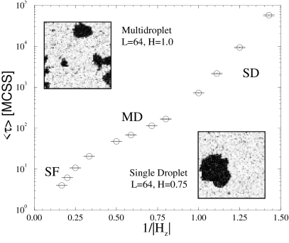
Figure 5: Switching behavior for an anisotropic $n=3$ Heisenberg model on a two-dimensional $L\times L$ square lattice. The parameters are $J_{x}=J_{y}=1$, $J_{z}=2$, and $T=1$, which is below the critical temperature for this model. The circles are for a system with $L=16$, and the single-droplet (SD), multidroplet (MD), and strong-field (SF) regimes are labeled. The insets show typical system configurations during the switching process for systems with $L=64$. Note that the dynamic spinodal (DSp) depends on $L$, and thus the SD and MD regimes appear at different fields for $L=16$ and $L=64$. The grayscale for the insets shows $s_{z}$ with lighter shades indicating metastable spins and darker shades indicating more stable spins

The simulation begins with all $\vec{s}_{i}=-\hat{\vec{z}}$ and $H_{z}>0$. This metastable phase then decays in a manner consistent with homogeneous nucleation and growth. However, unlike the Ising model, the continuous degrees of freedom add additional complications, such as effective long-range interactions between droplets. We have not yet attempted to quantify these differences. Figure 5 shows lifetimes and configuration snapshots in the single-droplet, multidroplet, and strong-field regimes for an anisotropic Heisenberg model at a temperature below criticality. The field dependence of the lifetime is seen to be very similar to that of the two-dimensional Ising model, shown in Fig. 3(a).

Finite-temperature Langevin Micromagnetics

[angle=00,width=.60]fig6_Pillar.ps

Figure 6: Magnetization along the pillar long axis, $M_{z}$, at three times during the switching process. Light shades represent the metastable orientation and dark shades the equilibrium orientation. The micromagnetic simulation shown in this figure models an individual pillar using a $7$ $\times$ $7$ $\times$ $49$ lattice at $T=20$ K. The pillar is shown in a one-quarter cut-away view

More realistic representations of nanoscale magnetic systems can be obtained by micromagnetic modeling. In this method the “spins” are coarse-grained magnetization vectors ${\vec{M}}({\vec{r}}_{i})$; each represents the magnetization within a cell centered at position ${\vec{r}_{i}}.$ In this low-temperature model GARA97 , the vectors have a fixed magnitude $M_{s}$ corresponding to the bulk saturation magnetization density. The time evolution of each spin is governed by the damped precessional motion given by the Landau-Lifshitz-Gilbert (LLG) equation BROW63B ; AHAI96

$$\frac{{\rm d}{\vec{M}}({\vec{r}}_{i})}{{\rm d}{t}}=\frac{\gamma_{0}}{1+\alpha^{2}}{\vec{M}}({\vec{r}}_{i})\times\left({\vec{H}}({\vec{r}}_{i})-\frac{\alpha}{M_{s}}{\vec{M}}({\vec{r}}_{i})\times{\vec{H}}({\vec{r}}_{i})\right)\;,$$ (8)

where the electron gyromagnetic ratio is $\gamma_{0}=1.76\times 10^{7}\;{\rm Hz/Oe}$ AHAI96 , and $\alpha$ is a phenomenological damping parameter. The local field at the $i$-th spin, ${\vec{H}}({\vec{r}}_{i})$, is generally different at each location. This field is a linear superposition of fields, one for each type of interaction in the system. Typical examples include fields from external sources, exchange, crystalline anisotropy, and dipole-dipole interactions. Thermal fluctuations may also contribute a term: a stochastic field ${\vec{H}}_{\rm n}({\vec{r}}_{i})$ that is assumed to fluctuate independently for each spin BROW63 . The fluctuations are assumed Gaussian, each with zero first moment and with the second moments given by the fluctuation-dissipation relation BROW63

$$\langle{{H}}_{{\rm n}\mu}({\vec{r}}_{i},{t}){{H}}_{{\rm n}\mu^{\prime}}({\vec{r}}_{i}^{\prime},{t}^{\prime})\rangle=\frac{2\alpha k_{\rm B}T}{\gamma_{0}M_{s}V}\delta\left({t}-{t}^{\prime}\right)\delta_{\mu,\mu^{\prime}}\delta_{i,i^{\prime}}\;,$$ (9)

where ${{H}}_{{\rm n}\mu}$ indicates one of the Cartesian components of $\vec{H}_{\rm n}$. Here $V=(\Delta{r})^{3}$ is the discretization volume of the cell, $\delta_{\mu,\mu^{\prime}}$ is the Kronecker delta representing the orthogonality of the Cartesian coordinates, and $\delta({t}-{t}^{\prime})$ is the Dirac delta function.

While this stochastic term necessitates careful treatment of the numerical integration in time of this stochastic differential (Langevin) equation, the most computationally intensive part of the calculation involves the dipole-dipole term. For systems with more than a few hundred model spins, it is necessary to use a sophisticated algorithm such as the fast multipole method (FMM) GREE87A ; GREE94 . An extensive discussion of the issues involved in finite-temperature simulations of micromagnetics is presented in BROW01 . The growth of a droplet during the switching of an iron nanopillar at $T$$=$$20\,{\rm K}$ is shown in Fig. 6. Nucleation is observed to occur at the ends of the pillars BROW01 .

3 Finite-temperature Micromagnetics Results for Nanoparticles

Micromagnetic simulations have been applied to the study of iron pillars modeled after those shown in Fig. 1. Unless otherwise noted, the model iron pillars discussed here are $5.2\,{\rm nm}$ $\times$ $5.2\,{\rm nm}$ $\times$ $88.4\,{\rm nm}$. The cross-sectional dimensions are small enough, about two exchange lengths, that the only significant inhomogeneities in the magnetization are those in the $z$ direction, i.e. along the long axis of the pillar HINZKE ; NOWAK2 .

[angle=00,width=.65]fig7_mm_pnot.eps

Figure 7: Probability of not switching before time $t$, $P_{\rm not}(t)$, for micromagnetic simulations at $T$$=$$100\,{\rm K}$ with applied fields of $1000\,{\rm Oe}$ and $800\,{\rm Oe}$ as labeled. The solid curves are simulation data for $624$ and $252$ switches, respectively, for pillars modeled as a one-dimensional chain of spins. The dashed curves are fits to the theoretical model, (10)

In light of this, the pillars have been modeled as a linear system of magnetic cubes with side $5.2\,{\rm nm}$. This model, discussed previously in BROW01 ; BOER97 , includes thermal fluctuations, exchange, and dipole-dipole interactions.

The results for $P_{\rm not}(t)$, with $T$$=$$100\,{\rm K}$ are shown in Fig. 7 for applied fields of $H$$=$$1000\,{\rm Oe}$ and $800\,{\rm Oe}$. Here switching is defined to occur when the $z$-component of the total magnetization, $M_{z}$, passes through zero. The form of $P_{\rm not}(t)$ is not exponential, which can be explained by the fact that nucleation of the reversed droplets is easier at the ends of the pillars than in the middle. Assuming that the nucleation rate for droplets at the end of the pillars is constant, $I$, and that the earliest time switching can occur because of the finite velocity of droplet growth is $t_{0},$ it can be shown that the probability of not switching is BROW01

$$P_{\rm not}\left(t\right)=\left\{\begin{array}[]{lr}1&t<t_{0}\\ e^{-2{I}(t-t_{0})}\left[1+2{I}(t-t_{0})\right]&t_{0}\leq t<2t_{0}\\ e^{-2{I}(t-t_{0})}\left[1+2{I}t_{0}\right]&{2t_{0}\leq t}\end{array}\right.\;.$$ (10)

The parameters are fitted by matching the first and second moments of the simulation results to those of the theoretical forms. As long as the applied field is relatively weak, the agreement between the theory and the simulations is quite good. Switching at times $t_{0}\leq t<2t_{0}$ is possible only when nucleation occurs at both ends.

Since the nucleation occurs at the ends, the dependence of the switching on the size of the system is different from that seen in isotropic models. Results for the parameters $t_{0}$ (squares) and $1/I$ (circles) at $T$$=$$100\,{\rm K}$ and $H$$=$$1000\,{\rm Oe}$ are shown in Fig. 8 for pillars of different lengths, i.e. composed of different numbers of cubes $5.2\,{\rm nm}$ on a side. The nucleation rate is nearly constant, indicating that the size of the energy barrier does not depend on the pillar length. The growth time, indicated by $t_{0}$, however, increases as the droplets have to grow farther to switch the magnetization. The nearly linear increase with pillar length indicates that the interface velocity is not significantly affected by the demagnetizing field associated with the high aspect ratio of the pillars.

[angle=00,width=.65]fig8_mm_vsL.eps

Figure 8: Inverse nucleation rate, $I^{-1}$, and earliest switching time, $t_{0}$, from (10), for different pillar lengths. The rate of nucleation at the ends of the pillars depends only weakly on the pillar length, and therefore likewise the energy barrier. The earliest switching time increases since the droplets have to grow for a longer time to switch longer pillars

Finally, changes in the switching mode as the field is changed are shown in Fig. 9. Here the mean switching time, $\langle t_{\rm sw}\rangle$, and standard deviation, $\sigma_{t}$, are shown versus applied field for the $88.4\,{\rm nm}$ long pillars at $T$$=$$100\,{\rm K}.$ The mean, $\langle t_{\rm sw}\rangle,$ and standard deviation, $\sigma_{t},$ of the switching time $t_{\rm sw}$ versus inverse applied field for pillars of the same type as considered in Fig. 7.

[angle=00,width=.65]fig9_mm_switch.eps

Figure 9: For very weak fields, $\langle t_{\rm sw}\rangle$ and $\sigma_{t}$ are equal, indicating an exponential probability density for the switching times in a single-droplet mode. At higher fields $\sigma_{t}$ decreases faster as the switching process becomes nearly deterministic. This is associated with the multidroplet switching mode

At weak fields the mean and standard deviation are nearly equal, where the exponential tail at $t>2t_{0}$ dominates (10). As the applied field is increased, the barrier to nucleation decreases, and the exponential behavior becomes less dominant. Eventually, (10) breaks down as the multidroplet reversal mechanism becomes important. The multidroplet nature of the reversal has been verified by direct observation of the switching, which shows droplets nucleating away from the ends at $H$$=$$1000\,{\rm Oe}.$

4 Hysteresis

Hysteresis is common in many nonlinear systems driven by an oscillating external force, including nanostructured magnets in an oscillating field. It occurs when the dynamics of the system is too sluggish to keep pace with the force. The term was coined by Ewing in the context of magnetoelasticity EWIN1881 from the Greek word husterein ($\stackrel{{\scriptstyle\scriptscriptstyle c}}{{\upsilon}}\!\!\sigma\tau\epsilon\rho\acute{\epsilon}\omega$) which means “to be behind.”

4.1 Hysteresis-loop Areas

[angle=0,width=.7]fig10_hystloop.eps

Figure 10: Hysteresis loop for one model Fe pillar of the same type considered in Fig. 7 at $T=100$ K for an oscillating field with a period of $75\,{\rm ns}$

Among the earliest aspects of hysteresis to receive sustained interest is the hysteresis-loop area. In the magnetic context of this article, the hysteresis loop is a plot of magnetization versus applied field, and its area is given by the integral $A=-\oint m(H){\rm d}H$. A typical hysteresis loop for a small system with thermal noise is shown in Fig. 10.

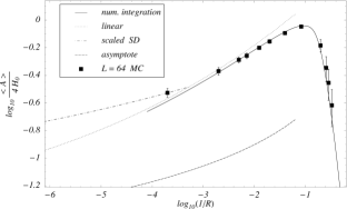
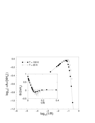
Figure 11: The hysteresis-loop area, $A$, versus the dimensionless frequency, $1/R$. (Top) Two-dimensional Ising model of an ultrathin film. Data points: Monte Carlo simulations for $L=64$, $T$$=$$0.8T_{c}$, and $H_{0}$$=$$0.3J$. For these parameters the magnetization switching occurs via the multidroplet mechanism, except for the lowest frequencies. Solid curve: numerical integration for sinusoidally varying field. Dotted curve: numerical integration for linearly varying field. Dot-dashed curve: numerical integration assuming magnetization reversal via the single-droplet mechanism. Dashed curve: low-frequency asymptotic solution. Power-law fits would yield very different effective exponents for fits centered at different frequencies. After SIDE99 . (Bottom) Micromagnetic model of iron pillars with length $88.4\,{\rm nm}$ and square cross-section $5.2\,{\rm nm}$ $\times$ $5.2\,{\rm nm}$ for $T$$=$$100\,{\rm K}$ (circles) and $T$$=$$20\,{\rm K}$ (squares) with $H_{0}$$=$$2000\,{\rm Oe}.$ The lines are guides to the eye. The inset shows the correlation between the magnetization and field versus frequency. The lowest-frequency zero-crossing, indicating a resonance condition, occurs at roughly the same frequency as the maximum in $A$

The particular importance of the loop area is that it corresponds to the energy dissipation per period of the applied field. It is thus relevant to the performance of most electrical and electronic equipment. Recent experiments on ultrathin Fe and Co films with Ising-like anisotropy have considered the frequency dependence of the hysteresis-loop areas HE93 ; JIAN95 ; SUEN97 ; SUEN99 . The results of these studies were interpreted in terms of power laws, but with exponents that vary widely between experiments. The experimental situation thus may appear somewhat unclear.

A resolution is provided by the nucleation-and-growth picture of magnetization switching presented here. We assume that the system is driven by a sinusoidally oscillating field, $H(t)=H_{0}\sin(\omega t)$. Since the nucleation rate, which has the dimension of a frequency per unit volume, is proportional to $\exp\left[-\beta\Xi(T)/|H|^{d-1}\right]$ by (1), one would expect that the field at which the magnetization changes sign should depend on the frequency as $-\left(\ln\omega\right)^{-1/(d-1)}$. The loop area is approximately proportional to the switching field multiplied by the saturation magnetization (see Fig. 10). Thus, one would expect the loop area to show this logarithmic frequency dependence in the asymptotic low-frequency limit. Analytic calculations have confirmed this asymptotic result. However, for higher, but still low, frequencies they show a very slow crossover to the asymptotic behavior, which is confirmed by Monte Carlo simulations. Such a slow crossover could easily be mistaken for a power law, even when observed over several decades in frequency SIDE99 ; SIDE98B ; SIDE98A . This result was shown to hold, both when the magnetization reversal occurs via the single-droplet mechanism SIDE98A and the multidroplet mechanism SIDE99 , even though the details are different. The behavior is illustrated in the top part of Fig. 11. Recently we have also found analogous behavior in micromagnetics simulations of nanometer-sized iron pillars, see the bottom part of Fig. 11. In these figures the frequency is given in terms of the dimensionless frequency $1/R=\omega\tau(H_{0},T)/2\pi$.

4.2 Dynamic Phase Transition

Different phenomena occur in hysteretic systems as the driving frequency is increased. Eventually the field will vary too quickly for the system to have time to switch during a single period.

Figure 12: The dynamic phase transition in a two-dimensional Ising system at $T=0.8T_{c}$, driven by a square-wave oscillating field of amplitude $H_{0}=0.3J$. After KORN00 . (a) The dynamic order parameter, $\langle|Q|\rangle$, versus the dimensionless period $R$ for several system sizes. (b) The order-parameter fluctuation strength, $X_{L}^{Q}$, versus $R$ for several system sizes

Thus, low frequencies lead to symmetric hysteresis loops, such as in Fig. 10, while high frequencies produce loops in which the magnetization oscillates about one or the other of its zero-field equilibrium values. For small systems or weak field amplitudes, such that the magnetization reversal occurs via the single-droplet mechanism, this results in stochastic resonance SIDE98A .

For large systems or stronger fields, such that the magnetization switching occurs via the multidroplet mechanism, the transition from symmetric to asymmetric hysteresis loops becomes a genuine critical phenomenon at a sharply defined critical frequency. The transition is essentially due to a competition between two time scales: the metastable lifetime, $\tau(H_{0},T)$, and the frequency of the applied field, $\omega/2\pi$. As a result, the critical value of the reduced frequency $1/R$ is on the order of unity. This nonequilibrium phase transition was first observed in numerical solutions of mean-field equations of motion for ferromagnets in oscillating fields TOME90 ; MEND91 . Subsequently it has been observed in numerous Monte Carlo simulations of kinetic Ising systems SIDE99 ; KORN00 ; LO90 ; ACHA94 ; ACHA95 ; ACHA97C ; ACHA97D ; ACHA98 ; CHAK99 ; BUEN98 ; BUEN00 ; SIDE98 and in further mean-field studies ACHA95 ; ACHA97D ; ACHA98 ; BUEN98 ; ZIMM93A . It may also have been experimentally observed in ultrathin films of Co on Cu(100) JIAN95 ; JIAN96 .

In this far-from-equilibrium phase transition the role of order parameter is played by the period-averaged magnetization, $Q=(\omega/2\pi)\oint m(t){\rm d}t$. This quantity is shown in Fig. 12(a) versus the dimensionless period $R$ for several system sizes. The order-parameter fluctuation strength, $X_{L}^{Q}=L^{2}\left[\langle Q^{2}\rangle-\langle|Q|\rangle^{2}\right]$, which corresponds to the susceptibility in an equilibrium system, is shown for several values of $L$ in Fig. 12(b). Both the order parameter and its fluctuations depend on $L$ in a way very similar to data from simulations of equilibrium phase transitions. And, indeed, formal finite-size scaling analysis of the Monte Carlo data SIDE99 ; KORN00 ; SIDE98 , as well as analytical arguments GRIN85 ; FUJI01 , have shown that this far-from-equilibrium phase transition belongs to the same universality class as the equilibrium phase transition in the Ising model in zero field. This is a quite remarkable result, as it extends the scope of an equilibrium universality class to a far-from equilibrium system.

5 Summary

In this article we have presented numerical and theoretical results on magnetization reversal and hysteresis in models of magnetic nanoparticles and ultrathin films. Models that were explicitly considered are kinetic Ising and classical Heisenberg models, which were studied by dynamic Monte Carlo simulations, and continuum-spin micromagnetics models, which were studied by finite-temperature Langevin-equation methods. The simulation results were interpreted within the context of nucleation theory, and it was shown how the reversal modes change from single-droplet to multidroplet upon increasing the strength of the applied field or the size of the system. Computer simulations of model systems such as those presented here enable one to study in detail the statistical properties of the reversal processes, as well as the time dependent internal magnetization structure. Such simulation results have now attained sufficient quality that they can fruitfully be compared with present and future experiments.

References

- (1) J.L. Dormann, D. Fiorani, eds.: Magnetic Properties of Fine Particles, (North Holland, New York 1992)
- (2) M.F. Crommie, C.P. Lutz, D.M. Eigler: Science 262, 218 (1993).
- (3) A.D. Kent, T.M. Shaw, S. von Molnár, D.D. Awschalom: Science 262, 1250 (1993)
- (4) A.D. Kent, S. von Molnár, S. Gider, D. D. Awschalom: J. Appl. Phys. 76, 6656 (1994)
- (5) W.W. Pai, J.D. Zhang, J.F. Wendelken, R.J. Warmack: J. Vacuum Science & Technology B 15, 785 (1997)
- (6) S. Gider et al.: Appl. Phys. Lett. 69, 3269 (1996)
- (7) H.N. Bertram: Theory of Magnetic Recording (Cambridge U. Press, Cambridge 1994)
- (8) S.Y. Chou, M.S. Wei, P.R. Krauss, P.B. Fischer: J. Appl. Phys. 76, 6673 (1994)
- (9) M.A. Novotny, P.A. Rikvold: ‘Magnetic Particles’. In: Encyclopedia of Electrical and Electronics Engineering, Vol. 12, ed. by J.G. Webster (Wiley, New York 1999) p. 64
- (10) P.A. Rikvold, M.A. Novotny, M. Kolesik, H.L. Richards: ‘Nucleation Theory of Magnetization Reversal in Nanoscale Ferromagnets’. In: Dynamical Phenomena in Unconventional Magnetic Systems, ed. by A.T. Skjeltorp, D. Sherrington (Kluwer, Dordrecht 1998) p. 307, and references therein
- (11) U. Nowak: ‘Thermally Activated Reversal in Magnetic Nanostructures’. In: Annual Review of Computational Physics IX, ed. by D. Stauffer (World Scientific, Singapore 2001) p. 105
- (12) G. Brown, M.A. Novotny, P.A. Rikvold: Phys. Rev. B 64, in press (2001), e-print cond-mat/0101477
- (13) J.J.M. Ruigrok, R. Coehorn, S.R. Cumpson, H.W. Kestern: J. Appl. Phys. 87, 5398 (2000)
- (14) D. Weller, M.F. Doerner: Ann. Rev. Mater. Sci. 30, 611 (2000)
- (15) T. Chang, J.-G. Zhu, J.H. Judy: J. Appl. Phys. 73, 6716 (1993).
- (16) H.L. Richards, S.W. Sides, M.A. Novotny, P.A. Rikvold: J. Magn. Magn. Mater. 150, 37 (1995)
- (17) P.A. Rikvold, B.M. Gorman: ‘Recent Results on the Decay of Metastable Phases’. In: Annual Reviews of Computational Physics I, ed. by D. Stauffer (World Scientific, Singapore 1994) p. 149, and references therein
- (18) L. Néel: Ann. Géophys. 5, 99 (1949)
- (19) W.F. Brown: J. Appl. Phys. 30, 130S (1959)
- (20) W.F. Brown: Phys. Rev. 130, 1677 (1963)
- (21) M. Kolesik, M.A. Novotny, P.A. Rikvold: Phys. Rev. B 56, 11790 (1997)
- (22) M. Kolesik, M.A. Novotny, P.A. Rikvold: Mater. Res. Soc. Conf. Proc. Ser. 492, 313 (1998)
- (23) P.A. Rikvold, M. Kolesik: J. Stat. Phys. 100, 377 (2000)
- (24) H.J. Hug et al.: J. Appl. Phys. 79, 5609 (1996)
- (25) R.H. Koch et al.: Phys. Rev. Lett. 84, 5419 (2000).
- (26) H.L. Richards, M.A. Novotny, P.A. Rikvold: Phys. Rev. B 54, 4113 (1996)
- (27) H.L. Richards et al.: Phys. Rev. B 55, 11521 (1997)
- (28) H. Tomita, S. Miyashita: Phys. Rev. B 46, 8886 (1992)
- (29) P.A. Rikvold, H. Tomita, S. Miyashita, S.W. Sides: Phys. Rev. E 49, 5080 (1994)
- (30) J.S. Langer: Ann. Phys. (N.Y.) 41, 108 (1967)
- (31) J.S. Langer: Ann. Phys. (N.Y.) 54, 258 (1969)
- (32) N.J. Günther, D.A. Nicole, D.J. Wallace: J. Phys. A 13, 1755 (1980)
- (33) M. Kolesik, M.A. Novotny, P.A. Rikvold: Phys. Rev. Lett. 80, 3384 (1998)
- (34) M. Kolesik, M.A. Novotny, P.A. Rikvold, D.M. Townsley: ‘Projected Dynamics for Metastable Decay in Ising Models’. In: Computer Simulation Studies in Condensed Matter Physics X, ed. by D.P. Landau, K.K. Mon, H.-B. Schüttler (Springer, Berlin 1998), p. 246
- (35) M.A. Novotny, M. Kolesik, P.A. Rikvold: Computer Phys. Commun. 121-122, 330 (1999)
- (36) R.H. Schonmann: Commun. Math. Phys. 161, 1 (1994)
- (37) A.N. Kolmogorov: Bull. Acad. Sci. USSR, Phys. Ser. 1, 355 (1937)
- (38) W.A. Johnson, R.F. Mehl: Trans. Am. Inst. Mining and Metallurgical Engineers 135, 416 (1939)
- (39) M. Avrami: J. Chem. Phys. 7, 1103 (1939); 8, 212 (1940); 9, 177 (1941)
- (40) J. Lee, M.A. Novotny, P.A. Rikvold: Phys. Rev. E 52, 356 (1995)
- (41) N. Metropolis et al.: J. Chem. Phys. 21, 1087 (1953)
- (42) R. J. Glauber: J. Math. Phys. 4, 294 (1963)
- (43) M.A. Novotny: Phys. Rev. Lett. 74, 1 (1995); erratum 75, 1424 (1995)
- (44) A.B. Bortz, M.H. Kalos, J.L. Lebowitz: J. Comput. Phys. 17, 10 (1975)
- (45) G.H. Gilmer: J. Crystal Growth 35, 15 (1976)
- (46) M.A. Novotny: Computers in Physics 9, 46 (1995)
- (47) D.A. Garanin: Phys. Rev. B 55, 3050 (1997)
- (48) W.F. Brown: Micromagnetics (Wiley, New York 1963)
- (49) A. Aharoni: Introduction to the Theory of Ferromagnetism (Clarendon, Oxford 1996)
- (50) L. Greengard, V. Rohklin: J. Comput. Phys. 73, 325 (1987)
- (51) L. Greengard: Science 265, 909 (1994)
- (52) D. Hinzke, U. Nowak: Comput. Phys. Commun. 122, 334 (1999)
- (53) U. Nowak, D. Hinzke: J. Appl. Phys. 85, 4337 (1999)
- (54) E. D. Boerner, H. N. Bertram: IEEE Trans. Magn. 33, 3052 (1997)
- (55) J. A. Ewing: Proc. R. Soc. London 33, 21 (1881)
- (56) S.W. Sides, P.A. Rikvold, M.A. Novotny: Phys. Rev. E 59, 2710 (1999)
- (57) Y.-L. He, G.-C. Wang: Phys. Rev. Lett. 70, 2336 (1993)
- (58) Q. Jiang, H.-N. Yang, G.-C. Wang: Phys. Rev. B 52, 14911 (1995)
- (59) J.H. Suen, J. L. Erskine: Phys. Rev. Lett. 78, 3567 (1997)
- (60) J.H. Suen, M.H. Lee, G. Teeter, J. L. Erskine: Phys. Rev. B 59, 4249 (1999)
- (61) S.W. Sides, P.A. Rikvold, M. A. Novotny: J. Appl. Phys. 83, 6494 (1998)
- (62) S.W. Sides, P.A. Rikvold, M.A. Novotny: Phys. Rev. E 57, 6512 (1998)
- (63) T. Tomé, M.J. de Oliveira: Phys. Rev. A 41, 4251 (1990)
- (64) J.F.F. Mendes, E.J.S. Lage: J. Stat. Phys. 64, 653 (1991)
- (65) G. Korniss, C.J. White, P.A. Rikvold, M.A. Novotny: Phys. Rev. E 63, 016120 (2001)
- (66) W.S. Lo, R.A. Pelcovits: Phys. Rev. A 42, 7471 (1990)
- (67) M. Acharyya, B.K. Chakrabarti: ‘Ising System in Oscillating Field: Hysteretic Response’. In: Annual Reviews of Computational Physics I, ed. by D. Stauffer (World Scientific, Singapore 1994) p. 107
- (68) M. Acharyya, B. Chakrabarti: Phys. Rev. B 52, 6550 (1995)
- (69) M. Acharyya: Phys. Rev. E 56, 1234 (1997)
- (70) M. Acharyya: Phys. Rev. E 56, 2407 (1997)
- (71) M. Acharyya: Phys. Rev. E 58, 179 (1998)
- (72) B. Chakrabarti, M. Acharyya: Rev. Mod. Phys. 71, 847 (1999)
- (73) G. M. Buendía, E. Machado: Phys. Rev. E 58, 1260 (1998)
- (74) G. M. Buendía, E. Machado: Phys. Rev. B 61, 14686 (2000)
- (75) S.W. Sides, P.A. Rikvold, M.A. Novotny: Phys. Rev. Lett. 81, 834 (1998)
- (76) M. Zimmer: Phys. Rev. E 47, 3950 (1993)
- (77) Q. Jiang, H.-N. Yang, G.-C. Wang: J. Appl. Phys. 79, 5122 (1996)
- (78) G. Grinstein, C. Jayaprakash, Y. He: Phys. Rev. Lett. 55, 2527 (1985)
- (79) H. Fujisaka, H. Tutu, P.A. Rikvold: Phys. Rev. E 63, 036109 (2001); erratum 63, 059903 (2001)