Quasi-Static Fractures in Disordered Media and Iterated Conformal Maps

Abstract

We study the geometrical characteristic of quasi-static fractures in disordered media, using iterated conformal maps to determine the evolution of the fracture pattern. This method allows an efficient and accurate solution of the Lamé equations without resorting to lattice models. Typical fracture patterns exhibit increased ramification due to the increase of the stress at the tips. We find the roughness exponent of the experimentally relevant backbone of the fracture pattern; it crosses over from about 0.5 for small scales to about 0.75 for large scales, in excellent agreement with experiments. We propose that this cross-over reflects the increased ramification of the fracture pattern.

Considerable amount of theoretical work 52Mus ; 86LL ; 99FM on fracture in disordered media is based on attempts to solve the equation of motion for an isotropic elastic body in the continuum limit

$$\rho\frac{\partial^{2}{\bf u}}{dt^{2}}=(\lambda+\mu){\bf\nabla}({\bf\nabla}\cdot{\bf u})+\mu\nabla^{2}{\bf u}\ .$$ (1)

Here ${\bf u}$ is the field describing the displacement of each mass point from its location in an unstrained body and $\rho$ is the density. The constants $\mu$ and $\lambda$ are the Lamé constants. In terms of the displacement field the elastic strain tensor is defined as

$$\epsilon_{ij}\equiv\frac{1}{2}\left(\frac{\partial u_{i}}{\partial x_{j}}+\frac{\partial u_{j}}{\partial x_{i}}\right)\ .$$ (2)

For the development of a crack the important object is the stress tensor, which in linear elasticity is written as

$$\sigma_{ij}\equiv\lambda\delta_{ij}\sum_{k}\epsilon_{kk}+2\mu\epsilon_{ij}\ .$$ (3)

When the stress component which is transverse to the interface of a crack exceeds a threshold value $\sigma_{c}$, the crack can develop. When the external load is such that the transverse stress exceeds only slightly the threshold value, the crack develops slowly, and one can neglect the second time-derivative in Eq. (1). This is the quasi-static limit, in which after each growth event one needs to recalculate the strain field by solving the Lamé equation

$$(\lambda+\mu){\bf\nabla}({\bf\nabla}\cdot{\bf u})+\mu\nabla^{2}{\bf u}=0\ .$$ (4)

In many previous works the problem was approached by discretizing Eq. (4) on a lattice 90HR ; 81Sle ; 93ML ; 00PCP . In this letter we offer a novel approach based on iterated conformal maps; this method turned out to be very useful in the context of fractal growth patterns 98HL ; 99DHOPSS ; 00DFHP ; 00DLP and it appears advantageous also for the present problem.

Although we can develop the approach in the full generality of Eq. (4), for the sake of clarity in this Letter we will consider mode III fracturing for which a 3-dimensional elastic medium is subjected to a finite shear stress $\sigma_{zy}\to\sigma_{\infty}$ as $y\to\pm\infty$. Such an applied stress will create a displacement field $u_{z}(x,y)$, $u_{x}=0$, $u_{y}=0$ in the medium. Despite the medium being three dimensional, therefore, the calculation of the strain and stress tensors are two dimensional.

We can describe a crack of arbitrary shape by its interface $\vec{x}(s)$, where $s$ is the arc length which is used to parameterize the contour. We wish to develop a quasi-static model 89BDL ; 90Ker for the time development of this fracture in which discrete events advance the interface with a normal velocity

$$v_{n}(s)=\alpha(\sigma_{zt}(s)-\sigma_{c})$$ (5)

if the transverse component of the stress tensor $\sigma_{zt}$ is greater than a critical yield value $\sigma_{c}$ for fracturing; otherwise no fracture propagation occurs. We will use the notation $(t,n)$ to describe respectively the transverse and normal directions at any point on the two-dimensional crack interface. Whenever the interface has more than one position $s$ for which $v_{n}(s)$ does not vanish, we will respect the disorder by choosing the next growth position randomly with a probability proportional to $v_{n}(s)$. This is similar to Diffusion Limited Aggregation (DLA) in which a particle is grown with a probability proportional to the gradient to the field. One should note that another model could be derived in which all eligible fracture sites are grown simultaneously, growing a whole layer whose local width is $v_{n}(s)$. This would be more akin to Laplacian growth algorithms, which in general give rise to clusters in a different universality class than DLA 01BDP . We prefer the first in order to take the disorder of the material explicitly into account.

In mode III fracture ${\bf\nabla}\cdot{\bf u}=0$, and the Lamé equation reduces to Laplace’s equation

$$\partial^{2}u_{z}/\partial x^{2}+\partial^{2}u_{z}/\partial y^{2}=0,$$ (6)

and therefore $u_{z}$ is the real part of an analytic function

$$\chi(z)=u_{z}(x,y)+i\xi_{z}(x,y)$$ (7)

where $z=x+iy$. The boundary conditions far from the crack and on the crack interface can be used to find this analytic function. It should be stated here that mode I and mode II fractures can be reduced to a bi-Laplacian equation; then one needs to determine two rather than one analytic functions. How to accomplish a growth model using iterated conformal maps for those cases will be shown in a forthcoming publication 01BLP .

Far from the crack as $y\rightarrow\pm\infty$ we know $\sigma_{zy}\rightarrow\sigma_{\infty}$ or using the stress/strain relationships Eq. 3 we find that $u_{z}\approx[\sigma_{\infty}/\mu]y$. Thus the analytic function must have the form 2.3

$$\chi(z)\rightarrow-i[\sigma_{\infty}/\mu]z\quad{\rm as}~{}|z|\rightarrow\infty\ .$$ (8)

Now on the boundary of the crack the normal stress vanishes, i.e.

$$0=\sigma_{zn}(s)=\partial_{n}u_{z}=-\partial_{t}\xi_{z}.$$ (9)

Since $\xi_{z}$ is constant on the boundary, we choose $\xi_{z}=0$, which in turn is a boundary condition making the analytic function $\chi(z)$ real on the boundary of the crack:

$$\chi(z(s))=\chi(z(s))^{*}\ .$$ (10)

The direct determination of the strain tensor for an arbitrary shaped (and evolving) crack is still difficult. We therefore proceed by turning to a mathematical complex plane $\omega$, in which the crack is forever circular and of unit radius. The strain field for such a crack is well known, being the real part of the function $\chi^{(0)}(\omega)$ where

$$\chi^{(0)}(\omega)=-i[\sigma_{\infty}/\mu](\omega-1/\omega)$$ (11)

This is the unique analytic function obeying the boundary conditions $\chi^{(0)}(\omega)\rightarrow-i[\sigma_{\infty}/\mu]\omega$ as $|\omega|\rightarrow\infty$, while on the unit circle $\chi^{(0)}(\exp i\theta)=\chi^{(0)}(\exp i\theta)^{*}$.

Now invoke a conformal map $z=\Phi^{(n)}(\omega)$ that maps the exterior of unit circle in the mathematical plane $\omega$ to the exterior of the crack in the physical plane $z$, after $n$ growth steps. This conformal map is univalent by construction, and therefore admits a Laurent expansion

$$\Phi^{(n)}(\omega)=F_{1}^{(n)}\omega+F_{0}^{(n)}+F_{-1}^{(n)}/\omega+F_{-2}^{(n)}/\omega^{2}+\cdots$$ (12)

Then the required analytic function $\chi^{(n)}(z)$ is given by the expression

$$\chi^{(n)}(z)=-i[F_{1}^{(n)}\sigma_{\infty}/\mu]\Big{(}{\Phi^{(n)}}^{-1}(z)-1/{\Phi^{(n)}}^{-1}(z)\Big{)}$$ (13)

From this we should compute now the transverse stress tensor:

$$\sigma_{zt}(s) = \mu~{}\partial_{t}u_{z}=\mu~{}\Re\frac{\partial\chi^{(n)}(z)}{\partial s}$$ (14)

$$= \mu~{}\Re[\frac{\partial\chi^{(n)}(\Phi^{(n)}(e^{i\theta}))}{\partial\theta}\frac{\partial\theta}{\partial s}]$$

$$= -\Re\frac{iF_{1}^{(n)}\sigma_{\infty}\frac{\partial}{\partial\theta}(e^{i\theta}-e^{-i\theta})}{|\Phi^{{}^{\prime}(n)}(e^{i\theta})|}$$

$$= 2\sigma_{\infty}F_{1}^{(n)}\frac{\cos\theta}{|\Phi^{{}^{\prime}(n)}(e^{i\theta})|}\ ,$$

on the boundary.

Finally we describe how $\Phi^{(n)}(\omega)$ is obtained. Suppose that $\Phi^{(n-1)}(\omega)$ is known, with $\Phi^{(0)}(\omega)$ being the identity, $\Phi^{(0)}(\omega)=\omega$. We first compute the transverse strain tensor $\sigma_{zt}(\theta)=2\sigma_{\infty}F_{1}^{(n-1)}\cos\theta/|\Phi^{{}^{\prime}(n-1)}(e^{-i\theta})|$. In order to grow according to the requirement (5), we should choose growth sites more often when $\Delta\sigma(\theta)\equiv\sigma_{zt}(\theta)-\sigma_{c}$ is larger. We therefore construct a probability density $P(\theta)$ on the unit circle $e^{i\theta}$ which satisfies

$$P(\theta)=\frac{|\Phi^{{}^{\prime}(n-1)}(e^{i\theta})|\Delta\sigma(\theta)\Theta(\Delta\sigma(\theta))}{\int_{0}^{2\pi}|\Phi^{{}^{\prime}(n-1)}(e^{i\tilde{\theta}})|\Delta\sigma(\tilde{\theta})\Theta(\Delta\sigma(\tilde{\theta}))d\tilde{\theta}}\ ,$$ (15)

where $\Theta(\Delta\sigma(\tilde{\theta}))$ is the Heaviside function, and $|\Phi^{{}^{\prime}(n-1)}(e^{i\theta})|$ is simply the Jacobian of the transformation from mathematical to physical plane. The next growth position, $\theta_{n}$ in the mathematical plane, is chosen randomly with respect to the probability $P(\theta)d\theta$. In this way the disorder of the medium is mirrored in the growth pattern. At the chosen position on the crack, i.e. $z=\Phi^{(n-1)}(e^{i\theta_{n}})$, we want to advance the crack with a region whose area is the typical process zone for the material that we analyze. According to 90HR the typical scale of the process zone is $K^{2}/\sigma^{2}_{c}$, where $K$ is a characteristic fracture toughness parameter. Denoting the typical area of the process zone by $\lambda_{0}$, we achieve growth with an auxiliary conformal map $\phi_{\lambda_{n},\theta_{n}}(\omega)$ that maps the unit circle to a unit circle with a bump of area $\lambda_{n}$ centered at $e^{i\theta_{n}}$. An example of such a map is given by 98HL :

$$\phi_{\lambda,0}(w)=w\left\{\frac{(1+\lambda)}{2w}(1+w)\right.$$

$$\left.\times\left[1+w+w\left(1+\frac{1}{w^{2}}-\frac{2}{w}\frac{1-\lambda}{1+\lambda}\right)^{1/2}\right]-1\right\}^{a}$$ (16)

$$\phi_{\lambda,\theta}(w)=e^{i\theta}\phi_{\lambda,0}(e^{-i\theta}w)\,,$$ (17)

Here the bump has an aspect ratio $a$, $0\leq a\leq 1$. In our work below we use $a=2/3$. To ensure a fixed size step in the physical domain we choose

$$\lambda_{n}=\frac{\lambda_{0}}{|{\Phi^{(n-1)}}^{\prime}(e^{i\theta_{n}})|^{2}}\ .$$ (18)

Finally the updated conformal map $\Phi^{(n)}$ is obtained as

$$\Phi^{(n)}(\omega)=\Phi^{(n-1)}(\phi_{\lambda_{n},\theta_{n}}(\omega))\ .$$ (19)

The recursive dynamics can be represented as iterations of the map $\phi_{\lambda_{n},\theta_{n}}(w)$,

$$\Phi^{(n)}(w)=\phi_{\lambda_{1},\theta_{1}}\circ\phi_{\lambda_{2},\theta_{2}}\circ\dots\circ\phi_{\lambda_{n},\theta_{n}}(\omega)\ .$$ (20)

Every given fracture is determined completely by the random itinerary $\{\theta_{i}\}_{i=1}^{n}$. Eqs.(14) together with (20) offer an analytic expression for the transverse stress field at any stage of the crack propagation.

Fig. 1 exhibits a typical fracture pattern that is obtained with this theory, with $\sigma_{\infty}=1$, after 10 000 growth events. The threshold value of $\sigma_{c}$ for the occurrence of the first event (cf. Eq.(14) is $\sigma_{c}=2$. We always implement the first event. For the next growth event the threshold is $\sigma_{c}=2.9401...$. We thus display in Fig.1 a cluster obtained with $\sigma_{c}=2.94$, to be as close as possible to the quasi-static limit. Nevertheless, one should observe that as the pattern develops, the stress at the active zone increases, and we get progressively away from the quasi-static limit. Indeed, as a result of this, for fixed boundary conditions at infinity, there are more and more values of $\theta$ for which Eq.(15) does not prohibit growth. Since the tips of the patterns are mapped by ${\Phi^{(n)}}^{-1}$ to larger and larger arcs on the unit circle, the support of the probability $P(\theta)$ increases, and the fracture pattern becomes more and more ramified as the process advances. The geometric characteristics of the fracture pattern are not invariant to the growth. For this reason it makes little sense to measure the fractal dimension of the pattern; this is not a stable characteristic, and it will change with the growth.

On the other hand, we should realize that the fracture pattern is not what is observed in typical experiments. When the fracture hits the boundaries of the sample, and the sample breaks into two parts, all the side-branches of the pattern remain hidden in the damaged material, and only the backbone of the fracture pattern appears as the surface of the broken parts. The backbone does not suffer from the geometric variability discussed above. In Fig. 2 we show the backbone of the pattern displayed in Fig. 1.

This backbone is representative of all the fracture patterns. we should note that in our theory there are not lateral boundaries, and the backbone shown does not suffer from finite size effects which may very well exist in experimental realizations.

In determining the roughness exponent of the backbone, we should note that a close examination of it reveals that it is not a graph. There are overhangs in this backbone, and since we deal with mode III fracturing, the two pieces of material can separate leaving these overhangs intact. Accordingly, one should not approach the roughness exponent using correlation function techniques; these may introduce serious errors when overhangs exist 95OPZ . Rather, we should measure, for any given $r$, the quantity 97Bou

$$h(r)\equiv\langle{\rm Max}\{y(r^{\prime})\}_{x<r^{\prime}<x+r}-{\rm Min}\{y(r^{\prime}\}_{x<r^{\prime}<x+r}\rangle_{x}\ .$$ (21)

The roughness exponent $\zeta$ is then obtained from

$$h(r)\sim r^{\zeta}\ ,$$ (22)

if this relation holds. To get good statistics we average, in addition to all $x$ for the same backbone, over many fracture patterns. The result of the analysis is shown in Fig. 3.

We find that the roughness exponent for the backbone exhibits a clear cross-over from 0.54 for shorter distances $r$ to 0.75 for larger distances. Within the error bars these results are in excellent agreement with the numbers quoted experimentally, see for example 97Bou . The short length scale exponent of order 0.5 is also in agreement with recent simulational results of a lattice model 00PCP (which is by definition a short length scale solution). Bouchaud 97Bou proposed that the cross-over stems from transition between slow and rapid fracture, from the “vicinity of the depinning transition” to the “moving phase” in her terms. Obviously, in our theory we solve the quasi-static equation all along, and there is no change of physics. Nevertheless, as we observed before, the fracture pattern begins with very low ramification when the stress field exceeds the threshold value only at few positions on the fracture interface. Later it evolves to a much more ramified pattern due to the increase of the stress fields at the tips of the mature pattern. The scaling properties of the backbone reflect this cross-over. We propose that this effect is responsible for the cross-over in the roughening exponent of the backbone. It is remarkable that in spite of the apparently different mode of fracture (mode III is difficult to realize experimentally) nevertheless the exponents appear extremely close to those recorded experimentally for other fracture modes. This supports the conjecture of universality proposed in 97Bou .

We have thus demonstrated that iterated conformal maps offer an efficient method for studying fracture patterns. Here we considered only mode III quasi-static patterns. The theory for mode I and mode II is available and will be presented elsewhere 01BLP . The generalization to dynamical scaling, in which Eq.(1) is considered including the time derivatives is akin to the transition from electrostatics to electrodynamics. This is still an attractive goal for the road ahead.

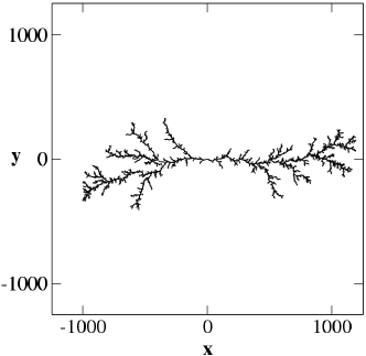
Figure 1: A typical fracture pattern that is obtained from iterated conformal maps. What is seen is the boundary of the fractured zone, which is the mapping of the unit circle in the mathematical domain onto the physical domain. Notice that the pattern becomes more and more ramified as the the fracture pattern develops. This is due to the enhancement of the stress field at the tips of the growing pattern

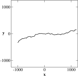
Figure 2: A typical backbone of the fracture pattern. This is the projection onto the x-y plane of the experimentally observed boundary between the two parts of the material that separate when the fracture pattern hits the lateral boundaries

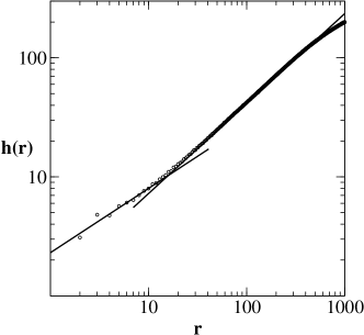
Figure 3: $h(r)$ averaged over all the backbone and over 70 fracture patterns each of which of 10 000 fracture events. There is a cross-over between a scaling law with roughness exponent $0.54\pm 0.05$ to and exponent of $0.75\pm 0.02$

References

- (1) N.I. Muskhelishvili, Some Basic Problems in the Mathematical Theory of Elasticity, (Noordhoff, Groningen, 1952).
- (2) L.D. Landau and E.M. Lifshitz, Theory of Elasticity, 3rd ed. (Pergamon, London, 1986).
- (3) J. Fineberg and M. Marder, Phys. Rep. 313, 1, (1999), and references therein.
- (4) H.J. Herrmann and S. Roux, Statistical Models for the Fracture of Disordered Media, (North Holland, Amsterdam, 1990), and references therein.
- (5) L. Slepian, Dov. Phys. Dokl. 26, 538 (1981).
- (6) M. Marder and X. Liu, Phys. Rev. Lett. 71, 2417 (1993).
- (7) A. Parisi, G. Caldarelli and L. Pietronero, arXiv:cond-mat/0004374
- (8) M.B. Hastings and L.S. Levitov, Physica D 116, 244 (1998).
- (9) B. Davidovitch, H.G.E. Hentschel, Z. Olami, I.Procaccia, L.M. Sander, and E. Somfai, Phys. Rev. E, 59 1368 (1999).
- (10) B. Davidovitch, M.J. Feigenbaum, H.G.E. Hentschel and I. Procaccia, Phys. Rev. E 62, 1706 (2000).
- (11) B. Davidovitch, A. Levermann, I. Procaccia, Phys. Rev. E, 62 R5919.
- (12) M. Barber, J. Donley and J. S. Langer, Phys. Rev. A40, 366 (1989)
- (13) See for example J. Kertész in 90HR .
- (14) F. Barra, B. Davidovitch and I. Procaccia, “Iterated Conformal Dynamics and Laplacian Growth”, submitted to Phys.Rev. E, also cond-mat/0105608.
- (15) F. Barra, A. Levermann and I. Procaccia, ”Solution of the bi-Laplacian Equation for Quasi-Static Mode I and Mode II Fracture Using Iterated Conformal Maps”, in preparation.
- (16) See for example 99FM Sect. 2.3.
- (17) Z. Olami, I. Procaccia and R. Zeitak, Phys. Rev. E52, 3402 (1995).
- (18) E. Bouchaud, J. Phys: Condens. Matter 9, 4319 (1997).