DC Josephson Effect in SNS Junctions of
Anisotropic Superconductors

Abstract

A formula for the Josephson current between two superconductors with anisotropic pairing symmetries is derived based on the mean-field theory of superconductivity. Zero-energy states formed at the junction interfaces is one of basic phenomena in anisotropic superconductor junctions. In the obtained formula, effects of the zero-energy states on the Josephson current are taken into account through the Andreev reflection coefficients of a quasiparticle. In low temperature regimes, the formula can describe an anomaly in the Josephson current which is a direct consequence of the exsitence of zero-energy states. It is possible to apply the formula to junctions consist of superconductors with spin-singlet Cooper pairs and those with spin-triplet Cooper pairs.

I introduction

The discoveries of the high-$T_{c}$ superconductors bednorz have stimulated an intensive research in this field. A symmetry of a Cooper pair is an important information to understand the mechanism of high-$T_{c}$ superconductivity. The Josephson effect in anisotropic superconductors has attracted considerable interst in recent years because high-$T_{c}$ superconductors may have the $d_{x^{2}-y^{2}}$-wave pairing symmetry sigrist ; wollman . So far, transport properties in various junctions of the $d$-wave superconductors have been discussed in a number of studies kashiwaya ; lofwander ; yip ; bruder ; kuklov ; barash ; tanaka ; samanta ; riedel ; golubov ; fogelstrom ; zhang ; zhu ; ohashi ; matsumoto ; nagato ; asano . In anisotropic superconductors, a sign of the pair potential depends on a direction of a quasiparticle’s motion. As a consequence, zero-energy states (ZES’s) hu are formed at the normal metal/ superconductor (NS) interface when the potential barrier at the interface is large enough. The ZES’s have been seen in the conductance spectra of tunnel junctions wei ; iguchi . It is known that the ZES’s cause a low-temperature anomaly of the Josephson current in SIS junctions of the $d$-wave superconductor barash ; tanaka .

The anisotropic superconductivity itself has been an important topic in condensed matter physics since unconventional superconductivity was found in heavy-fermion materials such as, CeCu₂Si₂, UBe₁₃ and UPt₃ steglich ; ott ; stewart . In a recent study, the anisotropic superconductivity was reported in a layered perovskite Sr₂RuO₄ maeno . Some of interesting effects of the anisotropy in the pairing symmetry on Josephson current are revealed in previous work geshkenbein ; millis ; sigrist2 . However, in order to study the contribution of the ZES’s to the Josephson current, we have to pay careful attention to a boundary condition of a wavefunction at the junction interface tanaka2 . Thus an expression of the Josephson current that describes the effects of the ZES’s is desirable to study an aspect of transport properties in anisotropic supercondutor junctions. So far, such formular for the Josephson current is obtained in SIS junctions of $d_{x^{2}-y^{2}}$ superconductors tanaka . However there is no general fomula which can be applied to junctions of spin-triplet superconductors.

In this paper, we derive a formula for the Josephson current in junctions of anisotropic superconductors with spin-singlet and spin-triplet Cooper pairs. The results are an extension of the Furusaki-Tsukada formula for $s$-wave superconductor junctions furusaki . Effects of the ZES’s on the Josephson current is naturally taken into account in the obtained formula through the Andreev reflection andreev coefficients (ARC’s) of a quasiparticle. The low-temperature anomaly in the Josephson current is described by the dependence of the ARC’s on temperatures. Throughout this paper, we take the units of $\hbar=k_{B}=1$, where $k_{B}$ is the Boltzmann constant.

This paper is organized as follows. In Sec. II, we derive the Josephson current formula based on the mean-field theory of superconductivity. In Sec. III, the formula is applied to junctions of superconductors with spin-singlet and spin-triplet Copper pairs. The conclusion is given in Sec. IV.

II Josephson Current Formula I

Let us consider SNS junctions as shown in Fig. 1, where the length of the normal metal is $L_{N}$ and the cross section of the junction is $S_{J}$. The (BCS) Hamiltonian in the mean-field approximation reads

$$H_{MF}= \frac{1}{2}\int\!\!d\boldsymbol{r}\int\!\!d\boldsymbol{r}^{\prime}\left[{\tilde{c}^{\dagger}(\boldsymbol{r})}\delta(\boldsymbol{r}-\boldsymbol{r}^{\prime}){\hat{h}}_{0}(\boldsymbol{r}^{\prime}){\tilde{c}(\boldsymbol{r}^{\prime})}\right.$$

$$-\tilde{c}^{t}(\boldsymbol{r})\delta(\boldsymbol{r}-\boldsymbol{r}^{\prime}){\hat{h}}^{\ast}_{0}(\boldsymbol{r}^{\prime})\left\{\tilde{c}^{\dagger}(\boldsymbol{r}^{\prime})\right\}^{t}$$

$$+{\tilde{c}^{\dagger}(\boldsymbol{r})}{\hat{\Delta}}(\boldsymbol{r}-\boldsymbol{r}^{\prime})\left\{{\tilde{c}^{\dagger}(\boldsymbol{r}^{\prime})}\right\}^{t}$$

$$-\left.{\tilde{c}^{t}(\boldsymbol{r})}{\hat{\Delta}}^{\ast}(\boldsymbol{r}-\boldsymbol{r}^{\prime}){\tilde{c}(\boldsymbol{r}^{\prime})}\right],$$ (1)

$${\hat{h}}_{0}(\boldsymbol{r})= \left[-\frac{\nabla^{2}}{2m}+V_{0}(\boldsymbol{r})-\mu_{F}\right]{\hat{\sigma}}_{0}+\boldsymbol{V}(\boldsymbol{r})\cdot{\hat{\boldsymbol{\sigma}}},$$ (2)

$${\tilde{c}(\boldsymbol{r})}\equiv \left(\begin{array}[]{c}c_{\uparrow}(\boldsymbol{r})\\ c_{\downarrow}(\boldsymbol{r})\end{array}\right),$$ (5)

where $c_{\sigma}(\boldsymbol{r})$ is the annihilation operator of an electron at $\boldsymbol{r}$ with spin $\sigma=\uparrow$ or $\downarrow$, $\left\{{\tilde{c}(\boldsymbol{r})}\right\}^{t}$ is the transpose of Eq. (5), $\hat{\sigma}_{0}$ is the unit matrix of $2\times 2$, and $\mu_{F}$ is the Fermi energy. Spin-independent potential is represented by $V_{0}(\boldsymbol{r})$ which includes the barrier potential at the two NS interfaces given by $V_{b}\left\{\delta(z)+\delta(z-L_{N})\right\}$. Spin-orbit scattering in the normal metal is denoted by $\boldsymbol{V}(\boldsymbol{r})\cdot{\hat{\boldsymbol{\sigma}}}$. A pair potential between an electron with ($\sigma$, $\boldsymbol{r}$) and that with ($\sigma^{\prime}$, $\boldsymbol{r}^{\prime}$) is described by $\Delta_{\sigma,\sigma^{\prime}}(\boldsymbol{r}-\boldsymbol{r}^{\prime})$. In the normal segment ($0<z<L_{N}$), the pair potential is taken to be zero. In what follows, $2\times 2$ matrices are indicated by $\widehat{\cdots}$. The pair potential is given by

$${\hat{\Delta}}(\boldsymbol{r})=\begin{cases}id_{0}(\boldsymbol{r})\hat{\sigma}_{2}&\text{ singlet }\\ i(\boldsymbol{d}(\boldsymbol{r})\cdot{\hat{\boldsymbol{\sigma}}})\hat{\sigma}_{2}&\text{ triplet },\end{cases}$$ (6)

where $\hat{\sigma}_{j}$ with $j=1,2$ and 3 are the Pauli’s matrices. The pair potential satisfies a relation

$$-{\hat{\Delta}}^{t}(\boldsymbol{r}^{\prime}-\boldsymbol{r})={\hat{\Delta}}(\boldsymbol{r}-\boldsymbol{r}^{\prime}).$$ (7)

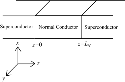
Figure 1: The SNS junction of anisotropic superconductors is illustrated. The phase of the pair potential on the left (right) superconductor is $\varphi_{L}$ ($\varphi_{R}$).

The Hamiltonian in Eq.(1) is diagonalized by the Bogoliubov transformation,

$$\left[\begin{array}[]{c}\tilde{c}(\boldsymbol{r})\\ \{\tilde{c}^{\dagger}(\boldsymbol{r})\}^{t}\end{array}\right]= \sum_{\lambda}\left[\begin{array}[]{cc}\hat{u}_{\lambda}(\boldsymbol{r})&\hat{v}_{\lambda}^{\ast}(\boldsymbol{r})\\ \hat{v}_{\lambda}(\boldsymbol{r})&\hat{u}_{\lambda}^{\ast}(\boldsymbol{r})\end{array}\right]\left[\begin{array}[]{c}\tilde{\alpha}_{\lambda}\\ \{\tilde{\alpha}_{\lambda}^{\dagger}\}^{t}\end{array}\right],$$ (14)

$$H_{MF}= \sum_{\lambda}\tilde{\alpha}^{\dagger}\,\hat{E}_{\lambda}\,\tilde{\alpha}_{\lambda},$$ (15)

$$\hat{E}_{\lambda}= \left[\begin{array}[]{cc}E_{\lambda,1}&0\\ 0&E_{\lambda,2}\end{array}\right],$$ (18)

where

$$\tilde{\alpha}_{\lambda}\equiv \left(\begin{array}[]{c}\alpha_{\lambda,\uparrow}\\ \alpha_{\lambda,\downarrow}\end{array}\right),$$ (21)

denotes the annihilation operator of a Bogoliubov quasiparticle. The wavefunctions satisfy the Bogoliubov-de Gennes (BdG) equation degennes ,

$$\displaystyle{\int} \!\!\!d\boldsymbol{r}^{\prime}\left[\begin{array}[]{cc}\delta(\boldsymbol{r}-\boldsymbol{r}^{\prime}){\hat{h}}_{0}(\boldsymbol{r}^{\prime})&\hat{\Delta}(\boldsymbol{r}-\boldsymbol{r}^{\prime})\\ -\hat{\Delta}^{\ast}(\boldsymbol{r}-\boldsymbol{r}^{\prime})&-\delta(\boldsymbol{r}-\boldsymbol{r}^{\prime}){\hat{h}}^{\ast}_{0}(\boldsymbol{r}^{\prime})\end{array}\right]$$ (24)

$$\times \left[\begin{array}[]{c}\hat{u}_{\lambda}(\boldsymbol{r}^{\prime})\\ \hat{v}_{\lambda}(\boldsymbol{r}^{\prime})\end{array}\right]=\left[\begin{array}[]{c}\hat{u}_{\lambda}(\boldsymbol{r})\\ \hat{v}_{\lambda}(\boldsymbol{r})\end{array}\right]\hat{E}_{\lambda}.$$ (29)

When the wavefunction

$$\left[\begin{array}[]{c}\hat{u}_{\lambda}(\boldsymbol{r})\\ \hat{v}_{\lambda}(\boldsymbol{r})\end{array}\right],$$ (30)

is belonging to a positive eigenvalue $\hat{E}_{\lambda}$, the wavefunction

$$\left[\begin{array}[]{c}\hat{v}_{\lambda}^{\ast}(\boldsymbol{r})\\ \hat{u}_{\lambda}^{\ast}(\boldsymbol{r})\end{array}\right],$$ (31)

is belonging to $-\hat{E}_{\lambda}$. They satisfy the following relations

$$\int d\boldsymbol{r}\left\{\hat{u}_{\lambda}^{\dagger}(\boldsymbol{r})\hat{u}_{\lambda^{\prime}}(\boldsymbol{r})+\hat{v}_{\lambda}^{\dagger}(\boldsymbol{r})\hat{v}_{\lambda^{\prime}}(\boldsymbol{r})\right\}= \delta_{\lambda,\lambda^{\prime}}\hat{\sigma}_{0},$$ (32)

$$\int d\boldsymbol{r}\left\{\hat{u}_{\lambda}^{\dagger}(\boldsymbol{r})\hat{v}_{\lambda^{\prime}}^{\ast}(\boldsymbol{r})+\hat{v}_{\lambda}^{\dagger}(\boldsymbol{r})\hat{u}_{\lambda^{\prime}}^{\ast}(\boldsymbol{r})\right\}= \hat{0},$$ (33)

$${\sum_{\lambda}}^{\prime}\left\{\hat{u}_{\lambda}(\boldsymbol{r})\hat{u}_{\lambda}^{\dagger}(\boldsymbol{r}^{\prime})+\hat{v}_{\lambda}^{\ast}(\boldsymbol{r})\hat{v}_{\lambda}^{t}(\boldsymbol{r}^{\prime})\right\}= \delta(\boldsymbol{r}-\boldsymbol{r}^{\prime})\hat{\sigma}_{0},$$ (34)

$${\sum_{\lambda}}^{\prime}\left\{\hat{u}_{\lambda}(\boldsymbol{r})\hat{v}_{\lambda}^{\dagger}(\boldsymbol{r}^{\prime})+\hat{v}_{\lambda}^{\ast}(\boldsymbol{r})\hat{u}_{\lambda}^{t}(\boldsymbol{r}^{\prime})\right\}= \hat{0},$$ (35)

where ${\sum_{\lambda}}^{\prime}$ is a summation over $\lambda$ with positive eigenvalues. The local charge density is defined by

$$P(\boldsymbol{r},\tilde{t})=-e\>{\tilde{c}}^{\dagger}(\boldsymbol{r},\tilde{t})\>{\tilde{c}}(\boldsymbol{r},\tilde{t}),$$ (36)

where $\tilde{t}$ is a time. The current conservation low implies,

$$\frac{\partial}{\partial\tilde{t}}P(\boldsymbol{r},\tilde{t})+\nabla\cdot\boldsymbol{J}(\boldsymbol{r},\tilde{t})=0.$$ (37)

The Josephson current between the two superconductors is calculated from the expectation value of Eq. (37)

$$\boldsymbol{J}(\boldsymbol{r})= \displaystyle{\frac{e}{4mi}}\lim_{\boldsymbol{r}^{\prime}\rightarrow\boldsymbol{r}}\left(\nabla_{\boldsymbol{r}^{\prime}}-\nabla_{\boldsymbol{r}}\right)T\sum_{\omega_{n}}\textrm{ Tr}\;\check{\cal G}_{\omega_{n}}(\boldsymbol{r},\boldsymbol{r}^{\prime}),$$ (38)

$$\check{\cal G}_{\omega_{n}}(\boldsymbol{r},\boldsymbol{r}^{\prime})= {\sum_{\lambda}}^{\prime}\left[\left[\begin{array}[]{c}\hat{u}_{\lambda}(\boldsymbol{r})\\ \hat{v}_{\lambda}(\boldsymbol{r})\end{array}\right]\left[i\omega_{n}\hat{\sigma}_{0}-\hat{E}_{\lambda}\right]^{-1}\left[\begin{array}[]{c}\hat{u}_{\lambda}(\boldsymbol{r}^{\prime})\\ \hat{v}_{\lambda}(\boldsymbol{r}^{\prime})\end{array}\right]^{\dagger}+\left[\begin{array}[]{c}\hat{v}_{\lambda}^{\ast}(\boldsymbol{r})\\ \hat{u}_{\lambda}^{\ast}(\boldsymbol{r})\end{array}\right]\left[i\omega_{n}\hat{\sigma}_{0}+\hat{E}_{\lambda}\right]^{-1}\left[\begin{array}[]{c}\hat{v}_{\lambda}^{\ast}(\boldsymbol{r}^{\prime})\\ \hat{u}_{\lambda}^{\ast}(\boldsymbol{r}^{\prime})\end{array}\right]^{\dagger}\right],$$ (47)

where $T$ is a temperature, $\check{\cal G}_{\omega_{n}}(\boldsymbol{r},\boldsymbol{r}^{\prime})$ is the Matsubara Green function of the SNS junctions and $\check{\cdots}$ indicates $4\times 4$ matrices. On the derivation of Eq. (38), we have assumed that the amplitude of the pair potential is much smaller than the Fermi energy $\mu_{F}$.

In the superconductors, we assume that the all potentials are uniform. Thus the BdG equation in Eq. (29) is given in the Fourier representation,

$$\left[\begin{array}[]{cc}\xi_{\boldsymbol{k}}\hat{\sigma}_{0}&\hat{\Delta}(\boldsymbol{k})\\ -\hat{\Delta}^{\ast}(-\boldsymbol{k})&-\xi_{\boldsymbol{k}}\hat{\sigma}_{0}\end{array}\right]\left[\begin{array}[]{c}\hat{u}_{\boldsymbol{k}}\\ \hat{v}_{\boldsymbol{k}}\end{array}\right]=\left[\begin{array}[]{c}\hat{u}_{\boldsymbol{k}}\\ \hat{v}_{\boldsymbol{k}}\end{array}\right]\hat{E}_{\boldsymbol{k}},$$ (48)

where $\xi_{\boldsymbol{k}}=\boldsymbol{k}^{2}/(2m)-\mu_{F}$ and

$$\hat{\Delta}(\boldsymbol{r}-\boldsymbol{r}^{\prime})= \sum_{\boldsymbol{k}}\hat{\Delta}(\boldsymbol{k})\textrm{ e}^{i\boldsymbol{k}\cdot(\boldsymbol{r}-\boldsymbol{r}^{\prime})},$$ (49)

$$\hat{\Delta}(\boldsymbol{k})= \begin{cases}id_{0}(\boldsymbol{k})\hat{\sigma}_{2}&\text{singlet}\\ i(\boldsymbol{d}(\boldsymbol{k})\cdot\hat{\boldsymbol{\sigma}})\hat{\sigma}_{2}&\textrm{triplet}\end{cases}.$$ (50)

Since relations

$$d_{0}(-\boldsymbol{k})= d_{0}(\boldsymbol{k}),$$ (51)

$$\boldsymbol{d}(-\boldsymbol{k})= -\boldsymbol{d}(\boldsymbol{k}),$$ (52)

are satisfied in the momentum space, one finds

$$-\hat{\Delta}^{t}(-\boldsymbol{k})=\hat{\Delta}(\boldsymbol{k}).$$ (53)

When $z<z^{\prime}\leq 0$, the Green function can be calculated as

$$\check{\cal G}_{\omega_{n}}(\boldsymbol{r},\boldsymbol{r}^{\prime})=-im\omega_{n}\sum_{\boldsymbol{p}}\chi_{\boldsymbol{p}}(\boldsymbol{\rho})\;\chi_{\boldsymbol{p}}^{\ast}(\boldsymbol{\rho}^{\prime})\check{\Phi}_{L}$$ (64)

$$\times \left[\left\{\left(\begin{array}[]{c}\hat{u}_{+}^{e}\\ \hat{v}_{+}^{e}\end{array}\right)\hat{K}_{p}(k^{e}_{+},z)+\left(\begin{array}[]{c}\hat{u}_{+}^{h}\\ \hat{v}_{+}^{h}\end{array}\right)\hat{K}_{p}(k^{h}_{+},z)\hat{a}_{1}+\left(\begin{array}[]{c}\hat{u}_{-}^{e}\\ \hat{v}_{-}^{e}\end{array}\right)\hat{K}_{p}(-k^{e}_{-},z)\hat{b}_{1}\right\}\hat{K}_{p}(-k^{e}_{+},z^{\prime})\left(\begin{array}[]{cc}k^{e}_{1,+}&0\\ 0&k^{e}_{2,+}\end{array}\right)^{-1}\hat{\Omega}_{+}^{-1}\left(\begin{array}[]{c}\hat{u}_{+}^{e}\\ \hat{v}_{+}^{e}\end{array}\right)^{\dagger}\right.$$

$$+ \left\{\left(\begin{array}[]{c}\hat{u}_{-}^{h}\\ \hat{v}_{-}^{h}\end{array}\right)\hat{K}_{p}(-k^{h}_{-},z)+\left(\begin{array}[]{c}\hat{u}_{-}^{e}\\ \hat{v}_{-}^{e}\end{array}\right)\hat{K}_{p}(-k^{e}_{-},z)\hat{a}_{2}\left(\begin{array}[]{c}\hat{u}_{+}^{h}\\ \hat{v}_{+}^{h}\end{array}\right)\hat{K}_{p}(k^{h}_{+},z)\hat{b}_{2}\right\}\left.\hat{K}_{p}(k^{h}_{-},z^{\prime})\left(\begin{array}[]{cc}k^{h}_{1,-}&0\\ 0&k^{h}_{2,-}\end{array}\right)^{-1}\hat{\Omega}_{-}^{-1}\left(\begin{array}[]{c}\hat{u}_{-}^{h}\\ \hat{v}_{-}^{h}\end{array}\right)^{\dagger}\right]$$ (75)

$$\times \check{\Phi}_{L}^{\ast},$$ (76)

with

$$k_{l,\pm}^{e}= \sqrt{2m(\mu_{F}-\epsilon(\boldsymbol{p})+i\Omega_{l,\pm})},$$ (77)

$$k_{l,\pm}^{h}= \sqrt{2m(\mu_{F}-\epsilon(\boldsymbol{p})-i\Omega_{l,\pm})},$$ (78)

$$\Omega_{l,\pm}= \sqrt{\omega_{n}^{2}+|\Delta_{l,\pm}|^{2}},$$ (79)

$$\epsilon(\boldsymbol{p})= \frac{\boldsymbol{p}^{2}}{2m},$$ (80)

$$d_{0,\pm}= d_{0}(\boldsymbol{p},\pm k_{z}),$$ (81)

$$\boldsymbol{d}_{\pm}= \boldsymbol{d}(\boldsymbol{p},\pm k_{z}),$$ (82)

$$\hat{\Delta}_{\pm}= \begin{cases}id_{0,\pm}\hat{\sigma}_{2}&\text{singlet}\\ i(\boldsymbol{d}_{\pm}\cdot\hat{\boldsymbol{\sigma}})\hat{\sigma}_{2}&\text{triplet}\end{cases},$$ (83)

$$\boldsymbol{q}_{\pm}= i\boldsymbol{d}_{\pm}\times\boldsymbol{d}_{\pm}^{\ast},$$ (84)

$$\hat{K}_{p}(k,z)= \left(\begin{array}[]{cc}\textrm{ e}^{ik_{1}z}&0\\ 0&\textrm{ e}^{ik_{2}z}\end{array}\right),$$ (87)

$$\hat{\Omega}_{\pm}= \left(\begin{array}[]{cc}\Omega_{1,\pm}&0\\ 0&\Omega_{2,\pm}\end{array}\right),$$ (90)

$$\check{\Phi}_{j}= \left(\begin{array}[]{cc}\textrm{ e}^{i\varphi_{j}}\hat{\sigma}_{0}&0\\ 0&\textrm{ e}^{-i\varphi_{j}}\hat{\sigma}_{0}\end{array}\right),$$ (93)

$$\chi_{\boldsymbol{p}}(\boldsymbol{\rho})= \frac{\exp(i\boldsymbol{p}\cdot\boldsymbol{\rho})}{\sqrt{S_{J}}},$$ (94)

where $\varphi_{j}$ for $j=L$ or $R$ is the phase of the superconductor, $\boldsymbol{p}=(k_{x},k_{y})$ and $\boldsymbol{\rho}=(x,y)$. The amplitude of the pair potential for unitary states is defined by

$$|\Delta_{l,\pm}|=|\Delta_{\pm}|=\begin{cases}|d_{0,\pm}|&\text{singlet}\\ |\boldsymbol{d}_{\pm}|&\text{triplet}\end{cases}.$$ (95)

In unitary states, these amplitudes are independent of $l$, where $l$ indicates the spin configuration of a quasiparticle. The amplitude of the pair potential depends on the spin configuration of a quasiparticle in nonunitary states,

$$|\Delta_{l,\pm}|=\begin{cases}\sqrt{|\boldsymbol{d}_{\pm}|^{2}+|\boldsymbol{q}_{\pm}|}&(l=1)\\ \sqrt{|\boldsymbol{d}_{\pm}|^{2}-|\boldsymbol{q}_{\pm}|}&(l=2)\end{cases}.$$ (96)

In Eqs. (77) and (78), $k^{e(h)}_{l,\pm}$ is the wavenumber in the electron (hole) branch for $l$-th spin state. In the following, we approximately describe these wavenumbers as $k^{e(h)}_{l,\pm}\approx k_{z}=\sqrt{2m(\mu_{F}-\epsilon(\boldsymbol{p}))}$ as shown in Eqs.(81) and (82), where $(\boldsymbol{p},\pm k_{z})$ is the wavenumber on the Fermi surface. The $l$-th column of

$$\left(\begin{array}[]{c}\hat{u}^{e(h)}_{\pm}\\ \hat{v}^{e(h)}_{\pm}\end{array}\right),$$ (97)

corresponds to the wavefunction of $l$-th spin state in the electron (hole) branch. The reflection coefficients from the left superconductor to the left superconductor are defined in a matrix form furusaki

$$\hat{a}_{j=1,2}= \left(\begin{array}[]{cc}a_{j}(1,1)&a_{j}(1,2)\\ a_{j}(2,1)&a_{j}(2,2)\end{array}\right),$$ (100)

$$\hat{b}_{j=1,2}= \left(\begin{array}[]{cc}b_{j}(1,1)&b_{j}(1,2)\\ b_{j}(2,1)&b_{j}(2,2)\end{array}\right).$$ (103)

The ARC from the $l$-th spin state in the electron (hole) branch to the $l^{\prime}$-th spin state in the hole (electron) branch is denoted by $\hat{a}_{1}(l^{\prime},l)$, ($\hat{a}_{2}(l^{\prime},l)$). In the same way, $\hat{b}_{1}(l^{\prime},l)$ ($\hat{b}_{2}(l^{\prime},l)$) is the normal reflection coefficient from the $l$-th spin state in the electron (hole) branch to the $l^{\prime}$-th spin state in the electron (hole) branch. These reflection coefficients depend on $\boldsymbol{p}$ which indicates the propagating channel at the left NS interface. Substituting Eq. (76) into Eq. (38), the Josephson current becomes

$$J= \frac{ie}{2}\sum_{\boldsymbol{p}}T\sum_{\omega_{n}}\textrm{ Tr}\;\;\omega_{n}$$

$$\times \left[\left(\begin{array}[]{c}\hat{u}^{h}_{+}\\ \hat{v}^{h}_{+}\end{array}\right)\hat{a}_{1}\hat{\Omega}_{+}^{-1}\left(\begin{array}[]{c}\hat{u}^{e}_{+}\\ \hat{v}^{e}_{+}\end{array}\right)^{\dagger}\right.$$ (108)

$$-\left.\left(\begin{array}[]{c}\hat{u}^{e}_{-}\\ \hat{v}^{e}_{-}\end{array}\right)\hat{a}_{2}\hat{\Omega}_{-}^{-1}\left(\begin{array}[]{c}\hat{u}^{h}_{-}\\ \hat{v}^{h}_{-}\end{array}\right)^{\dagger}\right].$$ (113)

The expression of the Josephson current in Eq. (113) nishida is an extension of the Furusaki-Tsukada formula furusaki for $s$-wave junctions.

Throughout this paper, we use a representation

$$\left(\begin{array}[]{c}\hat{u}^{e}_{\pm}\\ \hat{v}^{e}_{\pm}\end{array}\right)= \left(\begin{array}[]{c}{u}_{\pm}\hat{\sigma}_{0}\\ {v}_{\pm}\displaystyle{\frac{\hat{\Delta}_{\pm}^{\dagger}}{|\Delta_{\pm}|}}\end{array}\right),$$ (118)

$$\left(\begin{array}[]{c}\hat{u}^{h}_{\pm}\\ \hat{v}^{h}_{\pm}\end{array}\right)= \left(\begin{array}[]{c}{v}_{\pm}\displaystyle{\frac{\hat{\Delta}_{\pm}}{|\Delta_{\pm}|}}\\ {u}_{\pm}\hat{\sigma}_{0}\end{array}\right),$$ (123)

$$u_{\pm}= \sqrt{\frac{1}{2}\left(1+\frac{\Omega_{\pm}}{\omega_{n}}\right)},$$ (124)

$$v_{\pm}= \sqrt{\frac{1}{2}\left(1-\frac{\Omega_{\pm}}{\omega_{n}}\right)},$$ (125)

for unitary states. In unitary states, $\Delta_{l,\pm}$ is independent of $l$ because of $\boldsymbol{q}=0$. For nonunitary states sigrist2 , we use

$$\left(\begin{array}[]{c}\hat{u}^{e}_{\pm}\\ \hat{v}^{e}_{\pm}\end{array}\right)= \left(\begin{array}[]{c}\hat{u}_{\pm}\\ \hat{\Delta}_{\pm}^{\dagger}\hat{v}_{\pm}\end{array}\right),$$ (130)

$$\left(\begin{array}[]{c}\hat{u}^{h}_{\pm}\\ \hat{v}^{h}_{\pm}\end{array}\right)= \left(\begin{array}[]{c}\hat{\Delta}_{\pm}\hat{v}_{\pm}^{\ast}\\ \hat{u}_{\pm}^{\ast}\end{array}\right),$$ (135)

$$\hat{u}_{\pm}= Q_{\pm}\displaystyle{\sum_{l=1}^{2}u_{l,\pm}\hat{S}_{l,\pm}},$$ (136)

$$\hat{v}_{\pm}= Q_{\pm}\displaystyle{\sum_{l=1}^{2}v_{l,\pm}\frac{\hat{S}_{l,\pm}}{|\Delta_{l,\pm}|}},$$ (137)

$$u_{l,\pm}= \sqrt{\frac{1}{2}\left(1+\frac{\Omega_{l,\pm}}{\omega_{n}}\right)},$$ (138)

$$v_{l,\pm}= \sqrt{\frac{1}{2}\left(1-\frac{\Omega_{l,\pm}}{\omega_{n}}\right)},$$ (139)

$$(Q_{\pm})^{-2}= 8|\boldsymbol{q}_{\pm}|(|\boldsymbol{q}_{\pm}|+q_{3,\pm}),$$ (140)

$$\hat{S}_{l,\pm}= {\hat{P}}_{l,\pm}\cdot{\hat{t}}_{l},$$ (141)

$$\hat{P}_{1,\pm}= |\boldsymbol{q}_{\pm}|\hat{\sigma}_{0}+\boldsymbol{q}_{\pm}\cdot\hat{\boldsymbol{\sigma}},$$ (142)

$$\hat{P}_{2,\pm}= |\boldsymbol{q}_{\pm}|\hat{\sigma}_{0}-\boldsymbol{q}_{\pm}\cdot\hat{\boldsymbol{\sigma}},$$ (143)

$$\hat{t}_{1}= \hat{\sigma}_{0}+\hat{\sigma}_{3},$$ (144)

$$\hat{t}_{2}= \hat{\sigma}_{0}-\hat{\sigma}_{3}.$$ (145)

In this paper, we consider four reflection processes to calculate $\hat{a}_{1}$ and $\hat{a}_{2}$ as shown in Fig. 2 (a) and neglect all higher-order terms. This approximation is justified when the potential barrier at the NS interfaces is large enough and the transmission probability in the normal segment is low enough. Thus in the normal segment, insulators or dirty normal metals are assumed. In order to estimate $\hat{a}_{1}$ and $\hat{a}_{2}$, we calculate the transmission and the reflection coefficients at the single NS interface for fixed $\boldsymbol{p}$ as shown in Appendix A. The ARC’s in Fig. 2 (a) are given by

$$\hat{a}_{1}^{(1)}(\boldsymbol{p})= \sum_{\boldsymbol{p}^{\prime}}\hat{t}_{SN}^{hh}(\boldsymbol{p},L)\cdot\hat{t}^{h}_{\boldsymbol{p},\boldsymbol{p}^{\prime}}\cdot\hat{r}_{NN}^{he}(\boldsymbol{p}^{\prime},R)\cdot\hat{t}^{e}_{\boldsymbol{p}^{\prime},\boldsymbol{p}}\cdot\hat{t}_{NS}^{ee}(\boldsymbol{p},L),$$ (146)

$$\hat{a}_{1}^{(2)}(\boldsymbol{p})= \sum_{\boldsymbol{p}^{\prime}}\hat{t}_{SN}^{he}(\boldsymbol{p},L)\cdot\hat{t}^{e}_{\boldsymbol{p},\boldsymbol{p}^{\prime}}\cdot\;\hat{r}_{NN}^{eh}(\boldsymbol{p}^{\prime},R)\cdot\hat{t}^{h}_{\boldsymbol{p}^{\prime},\boldsymbol{p}}\cdot\hat{t}_{NS}^{he}(\boldsymbol{p},L),$$ (147)

$$\hat{a}_{2}^{(1)}(\boldsymbol{p})= \sum_{\boldsymbol{p}^{\prime}}\hat{t}_{SN}^{ee}(\boldsymbol{p},L)\cdot\hat{t}^{e}_{\boldsymbol{p},\boldsymbol{p}}\cdot\;\hat{r}_{NN}^{eh}(\boldsymbol{p}^{\prime},R)\cdot\hat{t}^{h}_{\boldsymbol{p}^{\prime},\boldsymbol{p}}\cdot\hat{t}_{NS}^{hh}(\boldsymbol{p},L),$$ (148)

$$\hat{a}_{2}^{(2)}(\boldsymbol{p})= \sum_{\boldsymbol{p}^{\prime}}\hat{t}_{SN}^{eh}(\boldsymbol{p},L)\cdot\hat{t}^{h}_{\boldsymbol{p},\boldsymbol{p}^{\prime}}\cdot\hat{r}_{NN}^{he}(\boldsymbol{p}^{\prime},R)\cdot\;\hat{t}^{e}_{\boldsymbol{p}^{\prime},\boldsymbol{p}}\cdot\hat{t}_{NS}^{eh}(\boldsymbol{p},L),$$ (149)

where $\hat{t}^{e(h)}_{\boldsymbol{p}^{\prime},\boldsymbol{p}}$ is the transmission coefficient of the electronlike (holelike) quasiparticle in the normal conductor, and $\boldsymbol{p}^{\prime}$ indicates the propagating channel at the right NS interface. The transmission coefficients in the normal metal are described by

$${\hat{t}}^{e}_{\boldsymbol{p}^{\prime},\boldsymbol{p}}= iv_{\boldsymbol{p}}\textrm{ e}^{-ik_{z}^{\prime}L_{N}}\int d{\boldsymbol{\rho}}\int d{\boldsymbol{\rho}}^{\prime}\,{\hat{\cal G}}_{\omega_{n}}^{N,e}({\boldsymbol{\rho}}^{\prime},L_{N};{\boldsymbol{\rho}},0)\chi_{\boldsymbol{p}^{\prime}}^{\ast}({\boldsymbol{\rho}}^{\prime})\chi_{\boldsymbol{p}}({\boldsymbol{\rho}}),$$ (150)

$${\hat{t}}^{h}_{\boldsymbol{p},\boldsymbol{p}^{\prime}}= iv_{\boldsymbol{p}^{\prime}}\textrm{ e}^{ik_{z}^{\prime}L_{N}}\int d{\boldsymbol{\rho}}\int d{\boldsymbol{\rho}}^{\prime}\,{\hat{\cal G}}_{\omega_{n}}^{N,h}(\boldsymbol{\rho},0;\boldsymbol{\rho}^{\prime},L_{N})\chi_{\boldsymbol{p}}^{\ast}(\boldsymbol{\rho})\chi_{\boldsymbol{p}^{\prime}}(\boldsymbol{\rho}^{\prime}),$$ (151)

where ${\hat{\cal G}}_{\omega_{n}}^{N,e(h)}(\boldsymbol{r},\boldsymbol{r}^{\prime})$ is the Green function of the normal conductor in the electron (hole) branch stone . The velocity of a quasiparicle in the $z$ direction is $v_{\textbf{p}}$ for the propagating channel with $\boldsymbol{p}$. We assume that the NS interface is sufficiently clean so that $\boldsymbol{p}$ and $\boldsymbol{p}^{\prime}$ are conserved while the transmission and the reflection at the interfaces. In $\hat{a}_{1}^{(1)}$ in Eq. (146), a quasiparticle-wave is initially incident into the normal segment from the left superconductor through the channel specified by $\boldsymbol{p}$. After the Andreev reflection at the right NS interface, we assume that the reflected wave transmits to the left superconductor through the initial channel of $\boldsymbol{p}$. This is because a quasiparicle in the normal segment has the retro property under the time reversal symmetry bennaker . The two ARC’s in Eq.(113) are given by $\hat{a}_{1}=\hat{a}_{1}^{(1)}+\hat{a}_{1}^{(2)}$ and $\hat{a}_{2}=\hat{a}_{2}^{(1)}+\hat{a}_{2}^{(2)}$.

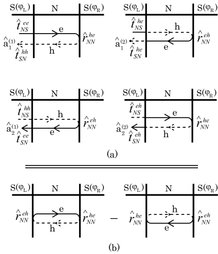
Figure 2: Four reflection processes in (a) contribute to the Josephson current. The Josephson current calculated from the four reflection processes in (a) is summarized in the reflection processes in (b).

By using Eqs. (113) and (146)-(149), we can derive a general expression of the Josephson current

$$J= ie\sum_{\boldsymbol{p}}\sum_{\boldsymbol{p}^{\prime}}T\sum_{\omega_{n}}\textrm{ Tr}$$

$$\times \left[\hat{r}_{NN}^{eh}(\boldsymbol{p},L)\cdot\hat{t}^{h}_{\boldsymbol{p},\boldsymbol{p}^{\prime}}\cdot\hat{r}_{NN}^{he}(\boldsymbol{p}^{\prime},R)\cdot\hat{t}^{e}_{\boldsymbol{p}^{\prime},\boldsymbol{p}}\right.$$

$$- \left.\hat{r}_{NN}^{he}(\boldsymbol{p},L)\cdot\hat{t}^{e}_{\boldsymbol{p},\boldsymbol{p}^{\prime}}\cdot\hat{r}_{NN}^{eh}(\boldsymbol{p}^{\prime},R)\cdot\hat{t}^{h}_{\boldsymbol{p}^{\prime},\boldsymbol{p}}\right].$$ (152)

The reflection processes in Eq. (152) are summarized in Fig. 2 (b). Since the relations

$$\hat{t}^{e}_{-\boldsymbol{p},-\boldsymbol{p}^{\prime}}= \left[\hat{t}^{h}_{\boldsymbol{p},\boldsymbol{p}^{\prime}}\right]^{\ast},$$ (153)

$$\hat{t}^{h}_{-\boldsymbol{p}^{\prime},-\boldsymbol{p}}= \left[\hat{t}^{e}_{\boldsymbol{p}^{\prime},\boldsymbol{p}}\right]^{\ast},$$ (154)

$$\hat{r}_{NN}^{eh}(-\boldsymbol{p},R)= \left\{\hat{r}_{NN}^{he}(\boldsymbol{p},R)\right\}^{\ast},$$ (155)

$$\hat{r}_{NN}^{he}(-\boldsymbol{p},L)= \left\{\hat{r}_{NN}^{eh}(\boldsymbol{p},L)\right\}^{\ast},$$ (156)

are satisfied (see Appendices A and B), the Josephson current results in

$$J= -2e\textrm{ Im}\sum_{\boldsymbol{p}}\sum_{\boldsymbol{p}^{\prime}}T\sum_{\omega_{n}}\textrm{ Tr}$$

$$\times \left[\hat{r}_{NN}^{eh}(\boldsymbol{p},L)\cdot\hat{t}^{h}_{\boldsymbol{p},\boldsymbol{p}^{\prime}}\cdot\hat{r}_{NN}^{he}(\boldsymbol{p}^{\prime},R)\cdot\hat{t}^{e}_{\boldsymbol{p}^{\prime},\boldsymbol{p}}\right].$$ (157)

The formula in Eq. (157) can be applied to various Josephson junctions. For instance, it is possible to calculate the Josephson current in clean SIS junctions by using a relation $\hat{t}^{e(h)}_{\boldsymbol{p},\boldsymbol{p}^{\prime}}\propto\delta_{\boldsymbol{p},\boldsymbol{p}^{\prime}}{\hat{\sigma}}_{0}$. We also note that the two superconductors are not necessary to be identical to each other.

III Josephson current formula II

In this section, we show the ARC’s of the superconductors in spin-singlet, spin-triplet unitary and spin-triplet nonunitary states because the Josephson current is described by the ARC’s at the NS interfaces in Eq. (157).

Firstly, we consider the superconductor with the spin-singlet Copper pairs. The ARC’s are given by

$${\hat{r}}_{NN}^{eh}(\boldsymbol{p},L)= -i{\hat{\Gamma}}_{su}(\boldsymbol{p},L)\textrm{ e}^{i\varphi_{L}},$$ (158)

$${\hat{r}}_{NN}^{he}(\boldsymbol{p},R)= -i{\hat{\Gamma}}_{su}^{\dagger}(\boldsymbol{p},R)\textrm{ e}^{-i\varphi_{R}},$$ (159)

$${\hat{\Gamma}}_{su}(\boldsymbol{p},j)= i\Gamma_{su}(\boldsymbol{p},j){\hat{\sigma}}_{2},$$ (160)

$$\Gamma_{su}(\boldsymbol{p},j)= \left.\frac{{\bar{k}}_{z}^{2}K_{+}d_{0,-}}{\Xi_{su}}\right|_{j},$$ (161)

$$\Xi_{su}= (H^{2}+{\bar{k}}_{z}^{2})d_{0,+}d_{0,-}+H^{2}K_{+}K_{-},$$ (162)

$$K_{\pm}= \Omega_{\pm}-|\omega_{n}|,$$ (163)

$${\bar{k}}_{z}= k_{z}/k_{F}$$ (164)

where $H=mV_{b}/k_{F}$ represents the strength of the potential barrier at the NS interface and $j=L$ or $R$ symbolically denote the character of the superconductors such as symmetries of the pair potential and orientation angles.

Secondly, the ARC’s in spin-triplet unitary states are given by

$${\hat{r}}_{NN}^{eh}(\boldsymbol{p},L)= -i{\hat{\Gamma}}_{tu}(\boldsymbol{p},L)\textrm{ e}^{i\varphi_{L}},$$ (165)

$${\hat{r}}_{NN}^{he}(\boldsymbol{p},R)= -i{\hat{\Gamma}}_{tu}^{\dagger}(\boldsymbol{p},R)\textrm{ e}^{-i\varphi_{R}},$$ (166)

$${\hat{\Gamma}}_{tu}(\boldsymbol{p},j)= i{\boldsymbol{\Gamma}}_{tu}(\boldsymbol{p},j)\cdot{\hat{\boldsymbol{\sigma}}}\;{\hat{\sigma}}_{2},$$ (167)

$${\boldsymbol{\Gamma}}_{tu}(\boldsymbol{p},j)= {\bar{k}}_{z}^{2}K_{+}$$

$$\!\!\!\!\!\!\!\!\!\!\!\!\!\!\!\!\!\!\!\times\left.\frac{\Xi_{tu}\boldsymbol{d}_{-}-(H^{2}+{\bar{k}}_{z}^{2})(\boldsymbol{d}_{+}^{\ast}\times\boldsymbol{d}_{-})\times\boldsymbol{d}_{-}}{\Xi_{tu}^{2}-\boldsymbol{D}_{tu}\cdot\boldsymbol{D}_{tu}}\right|_{j},$$ (168)

$$\Xi_{tu}= (H^{2}+{\bar{k}}_{z}^{2})\boldsymbol{d}_{+}^{\ast}\!\!\cdot\boldsymbol{d}_{-}\!\!+H^{2}K_{+}K_{-},$$ (169)

$$\boldsymbol{D}_{tu}= -i(H^{2}+{\bar{k}}_{z}^{2})(\boldsymbol{d}_{+}^{\ast}\times\boldsymbol{d}_{-}).$$ (170)

In unitary states, $\boldsymbol{d}_{\pm}$ often has a single component. In such case, one finds

$${\boldsymbol{\Gamma}}_{tu}(\boldsymbol{p},j)={\bar{k}}_{z}^{2}K_{+}\left.\frac{\boldsymbol{d}_{-}}{\Xi_{tu}}\right|_{j},$$ (171)

because of $\boldsymbol{d}_{+}^{\ast}\times\boldsymbol{d}_{-}=0$.

Finally we show the ARC’s in nonunitary states,

$${\hat{r}}_{NN}^{eh}(\boldsymbol{p},L)= -i{\hat{\Gamma}}_{nu}(\boldsymbol{p},L)\textrm{ e}^{i\varphi_{L}},$$ (172)

$${\hat{r}}_{NN}^{eh}(\boldsymbol{p},R)= -i{\hat{\Gamma}}_{nu}^{\dagger}(\boldsymbol{p},R)\textrm{ e}^{-i\varphi_{R}},$$ (173)

$${\hat{\Gamma}}_{nu}= i{\boldsymbol{\Gamma}}_{nu}(\boldsymbol{p},j)\cdot{\hat{\boldsymbol{\sigma}}}\;{\hat{\sigma}}_{2},$$ (174)

$${\boldsymbol{\Gamma}}_{nu}(\boldsymbol{p},j)= {\bar{k}}_{z}^{2}\left.\frac{\boldsymbol{D}_{nu}}{\boldsymbol{D}_{nu}\cdot\boldsymbol{D}_{nu}}\right|_{j},$$ (175)

$$\boldsymbol{D}_{nu}= (H^{2}+{\bar{k}}_{z}^{2})\left\{\frac{1}{2}\sum_{l}\frac{\boldsymbol{D}_{l,+}}{K_{l,+}}\right\}$$

$$+ H^{2}\left\{\frac{1}{2}\sum_{l}\frac{K_{l,-}\boldsymbol{D}_{l,+}}{|\Delta_{l,-}|^{2}}\right\},$$ (176)

$$\boldsymbol{D}_{1,\pm}= \boldsymbol{d}_{\pm}^{\ast}+i\frac{\boldsymbol{d}_{\pm}^{\ast}\times\boldsymbol{q}_{\pm}}{|\boldsymbol{q}_{\pm}|},$$ (177)

$$\boldsymbol{D}_{2,\pm}= \boldsymbol{d}_{\pm}^{\ast}-i\frac{\boldsymbol{d}_{\pm}^{\ast}\times\boldsymbol{q}_{\pm}}{|\boldsymbol{q}_{\pm}|},$$ (178)

$$K_{l,\pm}= \Omega_{l,\pm}-|\omega_{n}|.$$ (179)

Detail of the calculation is shown in Appendix A, where we derive the ARC’s of the superconductors in nonunitary states. We do not show the derivation for unitary states because it is much simpler than that in nonunitary states. As shown in above equations, the expression of the ARC’s in nonunitary states is very complicated. However if a relation

$$\boldsymbol{d}= \boldsymbol{d}_{+}=\nu\boldsymbol{d}_{-},$$ (180)

$$\nu= 1\,\,\textrm{ or}\,\,-1,$$ (181)

is satisfied, the ARC’s can be reduced to a rather simple expression

$${\hat{r}}_{NN}^{eh}(\boldsymbol{p},L)= \left.-i\left\{\frac{{\bar{k}}_{z}^{2}}{2|\boldsymbol{q}|}\sum_{l=1}^{2}\frac{{\hat{P}}_{l}}{\Xi_{nu}(l)}\right\}{\hat{\Delta}}\right|_{L}\!\!\!\!\textrm{ e}^{i\varphi_{L}},$$ (182)

$${\hat{r}}_{NN}^{he}(\boldsymbol{p},R)= \left.-i{\hat{\Delta}}^{\dagger}\left\{\frac{{\bar{k}}_{z}^{2}}{2|\boldsymbol{q}|}\sum_{l=1}^{2}\frac{{\hat{P}}_{l}}{\Xi_{nu}(l)}\right\}\right|_{R}\!\!\!\textrm{ e}^{-i\varphi_{R}},$$ (183)

$$\Xi_{nu}(l)= H^{2}\left\{(1-\nu)|\omega_{n}|+(1+\nu)\Omega_{l}\right\}$$

$$+{\bar{k}}_{z}^{2}(|\omega_{n}|+\Omega_{l}).$$ (184)

The effects of the ZES’s on the ARC’s can be easily confirmed in Eqs. (162), (169) and (184). For instance in Eq. (184), we find in the limit of $H>>1$ and $\omega_{n}\to 0$,

$$\Xi_{nu}(l)\to\begin{cases}2H^{2}|\Delta_{l}|&(\nu=1)\\ {\bar{k}}_{z}^{2}|\Delta_{l}|&(\nu=-1)\end{cases}.$$ (185)

In the absence of the ZES’s ($\nu=1$), the reflection coefficients proportional to $1/H^{2}$. On the other hand in the presence of the ZES’s ($\nu=-1$), the reflection coefficients are independent of the barrier height. In this way, the low-temperature anomaly of the Josephson current is described by the ARC’s.

In the normal metal, the two Green functions in Eqs. (150) and (151) satisfy a relation as shown in Appendix B,

$${\cal G}_{\omega_{n}}^{N,h}(\boldsymbol{r}^{\prime},\boldsymbol{r})=-{\hat{\sigma}}_{2}\left[\hat{\cal G}_{\omega_{n}}^{N,e}(\boldsymbol{r},\boldsymbol{r}^{\prime})\right]^{\dagger}{\hat{\sigma}}_{2},$$ (186)

because of the time reversal symmetry. The transmission coefficients can be parameterized by

$${\hat{\tau}}(\boldsymbol{p}^{\prime},\boldsymbol{p})\equiv \tau_{0}(\boldsymbol{p}^{\prime},\boldsymbol{p}){\hat{\sigma}_{0}}+{\boldsymbol{\tau}}(\boldsymbol{p}^{\prime},\boldsymbol{p})\cdot{\hat{\boldsymbol{\sigma}}},$$ (187)

$$= \sqrt{v_{\boldsymbol{p}}v_{\boldsymbol{p}^{\prime}}}\int d{\boldsymbol{\rho}}\int d{\boldsymbol{\rho}}^{\prime}\chi_{\boldsymbol{p}^{\prime}}^{\ast}({\boldsymbol{\rho}}^{\prime})\chi_{\boldsymbol{p}}({\boldsymbol{\rho}})$$

$$\times{\hat{\cal G}}_{\omega_{n}}^{N,e}({\boldsymbol{\rho}}^{\prime},L_{N};{\boldsymbol{\rho}},0).$$ (188)

Since the amplitude of the spin-orbit scattering is much smaller than that of the spin-independent transmission probability, we assume that

$$|\tau_{0}|\gg|{\boldsymbol{\tau}}|.$$ (189)

The conductance of the normal metal at $T=0$ is given by

$$G_{N}= \lim_{\omega_{n}\to 0}\frac{e^{2}}{h}\textrm{ Tr}\sum_{\boldsymbol{p},\boldsymbol{p}^{\prime}}{\hat{\tau}}(\boldsymbol{p}^{\prime},\boldsymbol{p}){\hat{\tau}}^{\dagger}(\boldsymbol{p}^{\prime},\boldsymbol{p}),$$ (190)

$$\simeq \lim_{\omega_{n}\to 0}\frac{2e^{2}}{h}\sum_{\boldsymbol{p},\boldsymbol{p}^{\prime}}|\tau_{0}(\boldsymbol{p}^{\prime},\boldsymbol{p})|^{2}.$$ (191)

By using Eq.(187), the Josephson current is rewritten as

$$J= -2e\textrm{ Im}\sum_{\boldsymbol{p}}\sum_{\boldsymbol{p}^{\prime}}T\sum_{\omega_{n}}\textrm{ Tr}$$

$$\times\left[\hat{r}_{NN}^{eh}(\boldsymbol{p},L)\cdot{\hat{\sigma}}_{2}\{\tau_{0}^{\ast}{\hat{\sigma}_{0}}+{\boldsymbol{\tau}}^{\ast}\cdot{\hat{\boldsymbol{\sigma}}}\}{\hat{\sigma}}_{2}\right.$$

$$\cdot\left.\hat{r}_{NN}^{he}(\boldsymbol{p}^{\prime},R)\cdot\{\tau_{0}{\hat{\sigma}_{0}}+{\boldsymbol{\tau}}\cdot{\hat{\boldsymbol{\sigma}}}\}\right].$$ (192)

Firstly we consider Josephson junctions where the two superconductors have the spin-singlet Cooper pairs. The Josephson current is given by

$$J_{SS}= 4e\sin\varphi T\sum_{\omega_{n}}\sum_{\boldsymbol{p},\boldsymbol{p}^{\prime}}$$

$$\times\Gamma_{su}(\boldsymbol{p}^{\prime},R)|\tau_{0}(\boldsymbol{p}^{\prime},\boldsymbol{p})|^{2}\Gamma_{su}(\boldsymbol{p},L),$$ (193)

where $\varphi=\varphi_{L}-\varphi_{R}$.

Secondly we consider junctions where spin-triplet and spin-singlet superconductors are on the left and on the right hand sides, respectively. The Josephson current results in

$$J_{TS}= 4eT\sum_{\omega_{n}}\sum_{\boldsymbol{p},\boldsymbol{p}^{\prime}}\textrm{Im}$$

$$\times \left[\textrm{ e}^{i\varphi}\Gamma_{su}(\boldsymbol{p}^{\prime},R)\boldsymbol{W}(\boldsymbol{p}^{\prime},\boldsymbol{p})\cdot{\boldsymbol{\Gamma}}_{t}(\boldsymbol{p},L)\right],$$ (194)

$$\boldsymbol{W}(\boldsymbol{p}^{\prime},\boldsymbol{p})= \left(\tau_{0}^{\ast}{\boldsymbol{\tau}}+\tau_{0}{\boldsymbol{\tau}}^{\ast}+i{\boldsymbol{\tau}}^{\ast}\times{\boldsymbol{\tau}}\right)(\boldsymbol{p}^{\prime},\boldsymbol{p}),$$ (195)

where ${\boldsymbol{\Gamma}}_{t}$ represents ${\boldsymbol{\Gamma}}_{tu}$ in Eq. (168) or ${\boldsymbol{\Gamma}}_{nu}$ in Eq. (175). As shown in Eq. (195), the $J_{TS}$ vanishes in the absence of the spin-orbit scattering in the normal metal geshkenbein ; millis ; sigrist2 .

Finally when the two superconductors have spin-triplet Cooper pairs, the Josephson current is given by

$$J_{TT}= 4eT\sum_{\omega_{n}}\sum_{\boldsymbol{p},\boldsymbol{p}^{\prime}}\textrm{ Im}$$

$$\times \left[\textrm{ e}^{i\varphi}{\boldsymbol{\Gamma}}_{t}(\boldsymbol{p},L)\cdot{\boldsymbol{\Gamma}}_{t}^{\ast}(\boldsymbol{p}^{\prime},R)|\tau_{0}(\boldsymbol{p}^{\prime},\boldsymbol{p})|^{2}\right].$$ (196)

The obtained formula in Eqs. (193), (194) and (196) are essentially the same as those in the previous results sigrist2 when the ZES’s are not formed at the NS interfaces. However in the presence of the ZES’s, the dependence of the Josephson current on temperatures in our results is drastically different from that in the previous one’s. This is because the ARC’s ( $\Gamma_{su}$, ${\boldsymbol{\Gamma}}_{tu}$ and ${\boldsymbol{\Gamma}}_{nu}$) describe the low-temperature anomaly of the Josephson current in the SNS junctions of anisotropic superconductors.

IV Conclusion

On the basis of the mean-field theory of the superconductivity, we derive a formula for the Josephson current between two anisotropic superconductors. The Josephson current is expressed by the Andreev reflection coefficients at the junction interfaces. The contribution of the zero-energy bound states formed at the NS interfaces to the Josephson current is taken into account through these Andreev reflection coefficients. The formula can be applied to SIS and SNS junctions of the anisotropic superconductors with spin-singlet and spin-triplet Copper pairs.

Appendix A Transmission and Reflection Coefficients at the NS interface

We derive the transmission and the reflection coefficients at the left NS interface ($z=0$), where the superconductor is in spin-triplet nonunitary states as shown in Fig. 3. In what follows, we calculate the coefficients after the analytic continuation (i.e., $E\rightarrow i\omega_{n}$) for $\omega_{n}>0$. In the normal metal, a wavefunction of a quasiparticle can be described by

$${\boldsymbol{\Psi}}^{N}_{\boldsymbol{p}}(\boldsymbol{\rho},z)=\left[\left(\begin{array}[]{c}\hat{\alpha}\\ \hat{0}\end{array}\right)\textrm{ e}^{-ik_{z}z}+\left(\begin{array}[]{c}\hat{0}\\ \hat{\beta}\end{array}\right)\textrm{ e}^{ik_{z}z}+\left(\begin{array}[]{c}\hat{A}\\ \hat{0}\end{array}\right)\textrm{ e}^{ik_{z}z}+\left(\begin{array}[]{c}\hat{0}\\ \hat{B}\end{array}\right)\textrm{ e}^{-ik_{z}z}\right]\chi_{\boldsymbol{p}}({\boldsymbol{\rho}}),$$ (197)

where $\hat{\alpha}$ and $\hat{\beta}$ ($\hat{A}$ and $\hat{B}$ ) are the amplitudes of incoming (outgoing) waves in the electron and the hole branches, respectively. In the same way, a wavefunction in the superconductor is given by

$${\boldsymbol{\Psi}}^{S}_{\boldsymbol{p}}(\boldsymbol{\rho},z)= \check{\Phi}_{L}\left[\left(\begin{array}[]{c}\hat{u}_{+}\\ \hat{\Delta}_{+}^{\dagger}\hat{v}_{+}\end{array}\right)\textrm{ e}^{ik_{z}z}\hat{\gamma}+\left(\begin{array}[]{c}\hat{\Delta}_{-}\hat{v}_{-}^{\ast}\\ \hat{u}_{-}^{\ast}\end{array}\right)\textrm{ e}^{-ik_{z}z}\hat{\delta}+\left(\begin{array}[]{c}\hat{u}_{-}\\ \hat{\Delta}_{-}^{\dagger}\hat{v}_{-}\end{array}\right)\textrm{ e}^{-ik_{z}z}\hat{C}\right.$$ (204)

$$+\left.\left(\begin{array}[]{c}\hat{\Delta}_{+}\hat{v}_{+}^{\ast}\\ \hat{u}_{+}^{\ast}\end{array}\right)\textrm{ e}^{ik_{z}z}\hat{D}\right]\chi_{\boldsymbol{p}}(\boldsymbol{\rho}),$$ (207)

where $\hat{\gamma}$ and $\hat{\delta}$ ($\hat{C}$ and $\hat{D}$ ) are the amplitudes of incoming (outgoing) waves in the electron and the hole branches, respectively. We note that $\hat{\alpha}$, $\hat{\beta}$, $\hat{\gamma}$ and $\hat{\delta}$ have only diagonal elements.

The two wavefunctions satisfy a continuity-condition at the left NS interface,

$${\boldsymbol{\Psi}}^{N}_{\boldsymbol{p}}(\boldsymbol{\rho},0)= {\boldsymbol{\Psi}}^{S}_{\boldsymbol{p}}(\boldsymbol{\rho},0),$$ (208)

$$\left.\frac{\partial}{\partial z}{\boldsymbol{\Psi}}^{N}_{\boldsymbol{p}}(\boldsymbol{\rho},z)\right|_{z=0}-2mV_{b}{\boldsymbol{\Psi}}^{N}_{\boldsymbol{p}}(\boldsymbol{\rho},0)= \left.\frac{\partial}{\partial z}{\boldsymbol{\Psi}}^{S}_{\boldsymbol{p}}(\boldsymbol{\rho},z)\right|_{z=0}.$$ (209)

From Eqs. (208) and (209), we obtain the transmission and the reflection coefficients

$$\hat{t}_{SN}^{ee}(\boldsymbol{p},L)= \bar{k}_{z}\,\kappa\,\hat{u}_{-}^{-1}\,\hat{Z}_{2}^{\dagger}\,\hat{\xi}_{2,+}^{\dagger}\,\textrm{ e}^{-i\varphi_{L}/2},$$ (210)

$$\hat{t}_{SN}^{eh}(\boldsymbol{p},L)= \bar{k}_{z}\,H\,\hat{u}_{-}^{-1}\,\hat{Z}_{2}^{\dagger}\,\textrm{ e}^{i\varphi_{L}/2},$$ (211)

$$\hat{t}_{SN}^{he}(\boldsymbol{p},L)= -\bar{k}_{z}\,H\,\left(\hat{u}_{+}^{\ast}\right)^{-1}\,\hat{Z}_{1}\,\textrm{ e}^{-i\varphi_{L}/2},$$ (212)

$$\hat{t}_{SN}^{hh}(\boldsymbol{p},L)= \bar{k}_{z}\,\kappa^{\ast}\,\left(\hat{u}_{+}^{\ast}\right)^{-1}\,\hat{Z}_{1}\,\hat{\xi}_{2,-}\,\textrm{ e}^{i\varphi_{L}/2},$$ (213)

$$\hat{r}_{SS}^{eh}(\boldsymbol{p},L)= -\hat{u}_{-}^{-1}\hat{\Delta}_{-}\,\hat{v}_{-}^{\ast}$$

$$-i\frac{H^{2}}{\omega_{n}}\,\hat{u}_{-}^{-1}\,\hat{Z}_{2}^{\dagger}\,\left(\hat{u}_{-}^{t}\right)^{-1}\hat{\Omega}_{-},$$ (214)

$$\hat{r}_{SS}^{he}(\boldsymbol{p},L)= -\left(\hat{u}_{+}^{\ast}\right)^{-1}\hat{\Delta}_{+}^{\dagger}\hat{v}_{+}$$

$$\!\!\!\!\!-i\frac{H^{2}}{\omega_{n}}\left(\hat{u}_{+}^{\ast}\right)^{-1}\hat{Z}_{1}\left(\hat{u}_{-}^{\dagger}\right)^{-1}\hat{\Omega}_{+},$$ (215)

$$\hat{r}_{NN}^{eh}(\boldsymbol{p},L)= -i{\bar{k}}_{z}^{2}\,\hat{Z}_{2}^{\dagger}\,\textrm{ e}^{i\varphi_{L}},$$ (216)

$$\hat{r}_{NN}^{he}(\boldsymbol{p},L)= -i\bar{k}_{z}^{2}\,\hat{Z}_{1}\,\textrm{ e}^{-i\varphi_{L}},$$ (217)

$$\hat{t}_{NS}^{ee}(\boldsymbol{p},L)= \frac{\bar{k}_{z}\kappa}{\omega_{n}}\,\hat{Z}_{2}^{\dagger}\,\hat{\xi}_{2,+}^{\dagger}\,\left(\hat{u}_{+}^{\dagger}\right)^{-1}\hat{\Omega}_{+}\textrm{ e}^{i\varphi_{L}/2},$$ (218)

$$\hat{t}_{NS}^{eh}(\boldsymbol{p},L)= -\frac{\bar{k}_{z}H}{\omega_{n}}\,\hat{Z}_{2}^{\dagger}\,\left(\hat{u}_{-}^{t}\right)^{-1}\hat{\Omega}_{-}\,\textrm{ e}^{i\varphi_{L}/2},$$ (219)

$$\hat{t}_{NS}^{he}(\boldsymbol{p},L)= \frac{\bar{k}_{z}H}{\omega_{n}}\,\hat{Z}_{1}\left(\hat{u}_{+}^{\dagger}\right)^{-1}\hat{\Omega}_{+}\,\textrm{ e}^{-i\varphi_{L}/2}$$ (220)

$$\hat{t}_{NS}^{hh}(\boldsymbol{p},L)= \frac{\bar{k}_{z}\kappa^{\ast}}{\omega_{n}}\,\hat{Z}_{1}\,\hat{\xi}_{2,-}\left(\hat{u}_{+}^{t}\right)^{-1}\hat{\Omega}_{-}\textrm{ e}^{-i\frac{\varphi_{L}}{2}},$$ (221)

$$\hat{r}_{NN}^{he}(-\boldsymbol{p},L)= \left[\hat{r}_{NN}^{eh}(\boldsymbol{p},L)\right]^{\ast}.$$ (222)

Here we define

$$\hat{\xi}_{1,\pm}= \left(\frac{1}{2|\boldsymbol{q}_{\pm}|}\sum_{l=1}^{2}\frac{K_{l,\pm}}{|\Delta_{l,\pm}|^{2}}\hat{P}_{l,\pm}\right)\hat{\Delta}_{\pm},$$ (223)

$$\hat{\xi}_{2,\pm}= \left(\frac{1}{2|\boldsymbol{q}_{\pm}|}\sum_{l=1}^{2}\frac{\hat{P}_{l,\pm}}{K_{l,\pm}}\right)\hat{\Delta}_{\pm},$$ (224)

$$\hat{Z}_{1}= \left[H^{2}\hat{\xi}_{1,+}+|\kappa|^{2}\hat{\xi}_{2,-}\right]^{-1},$$ (225)

$$\hat{Z}_{2}= \left[H^{2}\hat{\xi}_{1,-}+|\kappa|^{2}\hat{\xi}_{2,+}\right]^{-1},$$ (226)

$$\kappa= \bar{k}_{z}+iH.$$ (227)

In the same way, the ARC’s at the right NS interface are given by

$$\hat{r}_{NN}^{he}(\boldsymbol{p},R)= -i\bar{k}_{z}^{2}\,\hat{Z}_{2}\,\textrm{ e}^{-i\varphi_{R}},$$ (228)

$$\hat{r}_{NN}^{eh}(-\boldsymbol{p},R)= \left[\hat{r}_{NN}^{he}(\boldsymbol{p},R)\right]^{\ast}.$$ (229)

On the derivation, we use identities,

$$\hat{S}_{l,\pm}^{\dagger}\cdot\hat{S}_{l^{\prime},\pm}= \frac{\hat{t}_{l}}{2Q_{\pm}^{2}}\,\delta_{l,l^{\prime}},$$ (230)

$$\hat{S}_{l,\pm}\cdot\hat{S}_{l^{\prime},\pm}^{\dagger}= \frac{\hat{P}_{l,\pm}}{2|\boldsymbol{q}_{\pm}|Q_{\pm}^{2}}\,\delta_{l,l^{\prime}},$$ (231)

$$\hat{P}_{l,\pm}\cdot\hat{P}_{l^{\prime},\pm}= 2|\boldsymbol{q}_{\pm}|\hat{P}_{l,\pm}\,\delta_{l,l^{\prime}},$$ (232)

$$\hat{S}_{l,\pm}^{\dagger}\cdot\hat{\Delta}_{\pm}\cdot\hat{\Delta}^{\dagger}_{\pm}\cdot\hat{S}_{l^{\prime},\pm}= \frac{|\Delta_{l,\pm}|^{2}}{2Q^{2}_{\pm}}\,\hat{t}_{l}\,\delta_{l,l^{\prime}},$$ (233)

$$\hat{\Delta}^{\dagger}_{\pm}\cdot\hat{S}_{l,\pm}\cdot\hat{S}_{l^{\prime},\pm}^{\dagger}\cdot\hat{\Delta}_{\pm}= \frac{|\Delta_{l,\pm}|^{2}}{2|\boldsymbol{q}_{\pm}|Q^{2}_{\pm}}\,\hat{P}_{l,\pm}^{\ast}\,\delta_{l,l^{\prime}},$$ (234)

$$\hat{\Delta}_{\pm}\cdot\hat{P}_{l,\pm}^{\ast}= \hat{P}_{l,\pm}\cdot\hat{\Delta}_{\pm},$$ (235)

$$\hat{P}_{l,\pm}\cdot\hat{\Delta}_{\pm}\cdot\hat{\Delta}^{\dagger}_{\pm}= |\Delta_{l,\pm}|^{2}\hat{P}_{l,\pm}.$$ (236)

The ARC’s of superconductors in unitary states can be calculated in the same way. The derivation of the ARC’s in unitary states is much simpler than that in nonunitary states.

Figure 3: Amplitudes of incoming and outgoing waves at the left NS interface.

In addition to the four reflection processes shown in Fig. 2(a), six reflection processes can be considered for $\hat{a}_{1}$ and $\hat{a}_{2}$ as shown in Fig. 4. By using the coefficients in Eqs. (210)-(221), it is possible to show that these six processes do not contribute to the Josephson current.

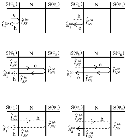
Figure 4: Reflection processes included in the coefficients $\hat{a}_{1}$ and $\hat{a}_{2}$. These processes, however, do not contribute to the Josephson current.

Appendix B Transmission coefficients in normal metal

Since the amplitude of the pair potential in the normal metal is taken to be zero, the BdG equation in Eq.(29) is decoupled into two equations,

$$\hat{h}_{0}(\boldsymbol{r})\hat{u}_{\lambda}= \hat{u}_{\lambda}\hat{E}_{\lambda}$$ (237)

$$-\hat{h}_{0}^{\ast}(\boldsymbol{r})\hat{v}_{\lambda}= \hat{v}_{\lambda}\hat{E}_{\lambda}.$$ (238)

The Green function in the normal metal obeys the equation,

$$(i\omega_{n}\hat{\sigma}_{0}-\hat{h}_{0}(\boldsymbol{r}))\hat{\cal G}_{\omega_{n}}^{N,e}(\boldsymbol{r},\boldsymbol{r}^{\prime})= \delta(\boldsymbol{r}-\boldsymbol{r}^{\prime})\hat{\sigma}_{0},$$ (239)

$$(i\omega_{n}\hat{\sigma}_{0}+\hat{h}_{0}^{\ast}(\boldsymbol{r}))\hat{\cal G}_{\omega_{n}}^{N,h}(\boldsymbol{r},\boldsymbol{r}^{\prime})= \delta(\boldsymbol{r}-\boldsymbol{r}^{\prime})\hat{\sigma}_{0}.$$ (240)

The Green function in the two branch are represented by

$$\hat{\cal G}_{\omega_{n}}^{N,e}(\boldsymbol{r},\boldsymbol{r}^{\prime})= \sum_{\lambda}\hat{u}_{\lambda}(\boldsymbol{r})\left[i\omega_{n}\hat{\sigma}_{0}-\hat{E}_{\lambda}\right]^{-1}\!\!\!\hat{u}_{\lambda}^{\dagger}(\boldsymbol{r}^{\prime}),$$ (241)

$$\hat{\cal G}_{\omega_{n}}^{N,h}(\boldsymbol{r},\boldsymbol{r}^{\prime})= -\left[\hat{\cal G}_{\omega_{n}}^{N,e}(\boldsymbol{r},\boldsymbol{r}^{\prime})\right]^{\ast},$$ (242)

where we use the complex conjugate of Eq. (237) for the Green function in the hole branch. By using Eqs.(150) and (151), we can show relations

$$\hat{t}_{-\boldsymbol{p},-\boldsymbol{p}^{\prime}}^{e}= \left[\hat{t}_{\boldsymbol{p},\boldsymbol{p}^{\prime}}^{h}\right]^{\ast},$$ (243)

$$\hat{t}_{-\boldsymbol{p}^{\prime},-\boldsymbol{p}}^{h}= \left[\hat{t}_{\boldsymbol{p}^{\prime},\boldsymbol{p}}^{e}\right]^{\ast}.$$ (244)

When the time-reversal symmetry holds in the normal metal, we find

$$\hat{h}_{0}^{\ast}(\boldsymbol{r})i\hat{\sigma}_{2}\hat{u}_{\lambda}=i\hat{\sigma}_{2}\hat{u}_{\lambda}\hat{E}_{\lambda}.$$ (245)

The Green function in the hole branch is described by that in the electron branch,

$$\hat{\cal G}_{\omega_{n}}^{N,h}(\boldsymbol{r}^{\prime},\boldsymbol{r})=-\hat{\sigma}_{2}\left[\hat{\cal G}_{\omega_{n}}^{N,e}(\boldsymbol{r},\boldsymbol{r}^{\prime})\right]^{\dagger}\hat{\sigma}_{2}.$$ (246)

References

• (1) J. G. Bednorz ans K. A. Müller, Z Phys. B 64, 189 (1986).
• (2) M. Sigrist and T. M. Rice, J. Phys. Soc. Jpn. 61, 4283 (1992); Rev. Mod. Phys. 67, 503 (1995).
• (3) D. A. Wollman, D. J. Van Harlingen, W. C. Lee, D. M. Ginsberg,and A. J. Leggett, Phys. Rev. Lett. 71, 2134 (1993).
• (4) S. Kashiwaya and Y. Tanaka, Rep. Prog. Phys. 63, 1641 (2001).
• (5) T. Löfwander, V. S. Shumeiko, and G. Wendin, Supercond. Sci. Technol. 14 R53 (2001).
• (6) S. Yip, Phys. Rev. B 52, 3087 (1995).
• (7) C. Bruder, A. van Otterlo, and G. T. Zimanyi, Phys. Rev. B 51, 12 904 (1995).
• (8) A. B. Kuklov, Phys. Rev. B 52, 6729 (1995).
• (9) Y. S. Barash, H. Burkhardt, and D. Rainer, Phys. Rev. Lett. 77, 4070 (1996).
• (10) Y. Tanaka and S. Kashiwaya, Phys. Rev. B 53, R11957 (1996).
• (11) M. P. Samanta and S. Datta, Phys. Rev. B 55, R8689 (1997).
• (12) R. A. Riedel and P. F. Bagwell, Phys. Rev. B 57, 6084 (1998).
• (13) A. A. Golubov, M. Y. Kupriyanov, Pis’ma Zh. Eksp. Teor. fiz 69, 242 (1999).[ Sov. Phys. JETP Lett. 69, 262 (1999).]
• (14) M. Fogelstöm, S. Yip, and J. Kurkijärvi, Physica C 294, 289 (1998).
• (15) W. Zhang, Phys. Rev. B 52, 3772 (1995).
• (16) J. -X. Zhu, Z. D. Wang, and H. X. Tang, Phys. Rev. B 54, 7354 (1996).
• (17) Y. Ohashi, J. Phys. Soc. Jpn. 65, 823 (1996).
• (18) M. Matsumoto and H. Shiba, J. Phys. Soc. Jpn. 64, 4867 (1995).
• (19) Y. Nagato and K. Nagai, Phys. Rev. B 51, 16254 (1995).
• (20) Y. Asano, Phys. Rev. B, 63, 052512 (2001); Phys. Rev. B, 64, 014511 (2001).
• (21) C. R. Hu, Phys. Rev. Lett. 72, 1526 (1994).
• (22) J. Y. T. Wei, N. -C. Yeh, D. F. Garrigus, and M. Strasik, Phys. Rev. Lett. 81, 2542 (1998).
• (23) I. Iguchi, W. Wang, M. Yamazaki, Y. Tanaka, and S. Kashiwaya, Phys. Rev. B 62, R6131 (2000); Y. Tanaka and S. Kashiwaya, Phys. Rev. Lett. 74, 3451 (1995).
• (24) E. Il’ichev, V. Zakosarenko, R. P. J. IJsselsteijn, V. Schultze, H. -G. Meyer, H. E. Hoenig, H. Hilgenkamp, and J. Mannhart, Phys. Rev. Lett. 81, 894 (1998); E. Il’ichev, M. Grajcar, R. Hlubina, R. P. J. IJsselsteijn, H. E. Hoenig, H. -G. Meyer, A. Golubov, M. H. S. Amin, A. M. Zagoskin. A. N. Omelyanchouk, and M. Yu. Kupriyanov, Phys. Rev. Lett. 86, 5369 (2001).
• (25) F. Steglich, J. Aarts, C. D. Bredl, W. Lieke, D. Meschede, W. Franz, and H. Schäfer, Phys. Rev. Lett. 43, 1892 (1979).
• (26) H. R. Ott, H. Rudigier, Z. Fisk, and J. L. Smith, Phys. Rev. Lett. 50, 1595 (1983).
• (27) G. R. Stewart, Z. Fisk, J. O. Willis, and J. L. Smith, Phys. Rev. Lett. 52, 679 (1984).
• (28) Y. Maeno, H. Hashimoto, K. Yoshida, S. Nishizaki, T. Fujita, J. G. Bednorz, and F. Lichtenberg, Nature 372, 532 (1994).
• (29) V.B. Geshkenbein and A.I. Larkin, Pis’ma Zh. Eksp. Teor. Fiz. 43, 306 (1986) [JETP Lett. 43, 395 (1986)].
• (30) A. Millis, D. Rainer, and J. A. Sauls, Phys. Rev. B 38, 4504 (1988).
• (31) M. Sigrist and K. Ueda, Rev. Mod. Phys. 63, 239 (1991).
• (32) Y. Tanaka ans S. Kashiwaya, J. Phys. Soc. Jpn. 69, 1152 (2000).
• (33) A. Furusaki and M. Tsukada, Solid State Commun. 78, 299 (1991).
• (34) After submission, we knew a theory reporting the Josephson current formula in a similar system of unitary states. M. Nishida, N. Hatakenaka, and S. Kurihara, cond-mat/0108368.
• (35) A. F. Andreev, Zh. Eksp. Theor. Fiz, 46,1823 (1964) [Sov. Phys. JETP 19, 1228 (1964)].
• (36) P. G. de Gennes, Superconductivity of Metals and Alloys, (Benjamin, New York, 1966).
• (37) A. D. Stone and A. Szafer, IBM J. Res. Develop. 32, 384 (1988).
• (38) C. W. J. Beenakker, J. A. Melsen, and P. W. Brouwer, Phys. Rev. B 51, 13883 (1995).