Generalized thermostatistics and Kolmogorov-Nagumo averages

Abstract

We introduce a generalized thermostatistics based on Kolmogorov-Nagumo averages and appropriately selected information measures. The formalism includes Tsallis non-extensive thermostatistics, but also extensive thermostatistics based on Rényi entropy. The Curie-Weiss model is discussed as an example.

Keywords: generalized thermostatistics, Kolmogorov-Nagumo mean, Rényi entropy, Tsallis entropy, kappa distribution, nonlinear averages, non-extensive thermodynamics, mean-field model.

1 Introduction

We present a thermostatistical theory based on the notion of Kolmogorov-Nagumo (KN) mean [10]. It deals with the problem of maximizing average information content under the constraint that the (nonlinear) average of some energy function has a given value.

From the point of view of information theory and the principle of maximal entropy [6] there are at least two ways to generalize the Boltzmann-Gibbs formalism of statistical mechanics. One can modify the definition of entropy/information, or one can modify the definition of average energy. We will make use of both possibilities. Many definitions of entropy can be found in literature [11]. In contrast, KN-averages, although known in statistics since many years, appear not to be used in the context of physics. Therefore, we will discuss in detail how they fit with basic principles of statistical mechanics.

Originally, our plan was to generalize the Boltzmann-Gibbs formalism by replacing Shannon’s entropy by Rényi’s $\alpha$-entropies, and by simultaneously replacing the usual linear statistical average by an appropriate KN-average. The resulting formalism is what we call Rényi thermostatistics in the sequel. However, the formalism allows further generalization which consists of replacing Rényi entropies by equivalent entropies, each time choosing appropriate KN-averages. By equivalent entropies we mean monotonically increasing continuous functions of Rényi entropies. Indeed, replacing an entropy by an equivalent one does not change the maximum entropy problem. One such entropy which is equivalent with Rényi’s, and which is quoted often in literature, is Tsallis’ entropy [13], studied earlier by Harvda and Charvat [7] and by Daróczy [8]. The thermostatistics which we propose is not equivalent with the non-extensive thermostatistics proposed by the Tsallis school because of the non-linear averages used in the present paper. Rényi thermostatistics is extensive, as we will show. The more general formalism can be non-extensive, and, in fact, comprises Tsallis’ thermostatistics as a special case.

Note that throughout the paper units are used in which Boltzmann’s constant $k_{B}$ equals one.

The paper is organized as follows. In section 2 the general formalism is explained. The standard Boltzmann-Gibbs formalism and some other formalisms are shown to be special cases. In section 3 equilibrium distributions are discussed. Special attention is paid to the definition of thermodynamic temperature. Section 4 shows how nonlinear averages fit with the fundaments of statistical mechanics. The Curie-Weiss model is treated as an example. Section 5 deals with Rényi thermostatistics and its obvious non-extensive generalization. The Curie-Weiss model serves again as an example, together with the two-level system. The last section contains a short discussion of our results. Throughout the paper we use deformed exponential and logarithmic functions with a definition which is broader than that found in literature. Details about these are found in appendix.

2 A general formalism

2.1 Optimization problem

For simplicity we restrict ourselves initially to functions $f(k)$ with integer $k=0,1,2,\cdots$. We use the index notation $f_{k}$.

The Kolmogorov-Nagumo (KN) average [3, 4] depends on a monotonically increasing function $\phi(x)$ and on parameters $p_{k}$. Essential for the present approach is that the latter are probabilities satisfying $p_{k}\geq 0$ and $\sum_{k}p_{k}=1$. The definition is

$$\langle f\rangle=\phi^{-1}\left(\sum_{k}p_{k}\phi(f_{k}).\right)$$ (1)

We will not make use of the possibility that $\phi$ may be decreasing instead of increasing.

Fix an additional monotonically increasing function $\omega(x)$. It is used to define information content $I_{k}$ by

$$I_{k}=\omega(1/p_{k}).$$ (2)

Because $\omega$ is increasing, less probable events (i.e. smaller $p_{k}$) carry more information. The average information content is now given by

$$\langle I\rangle=\phi^{-1}\left(\sum_{k}p_{k}\phi(\omega(1/p_{k}))\right).$$ (3)

Generalized thermostatistics studies the problem of maximizing average information content under the condition that average values of functions $f_{1}(x),\cdots f_{n}(x)$ have predetermined values $y_{1},\cdots,y_{n}$

$$\langle f_{j}\rangle=y_{j}\qquad\hbox{ for }j=1,2,\cdots,n.$$ (4)

Throughout the paper we consider the optimization problem with exactly one constraint, i.e., we fix some real function $\beta_{0}E_{k}$ and optimize information content under the condition that $\langle\beta_{0}E\rangle$ has a predetermined value $\beta_{0}U$. It is tradition to call $E_{k}$ the energy functional and to call $U$ the internal energy. Note that we introduce here a constant $\beta_{0}$ with dimension of inverse energy. Its first purpose is to make quantities dimensionless. Its actual role in the theory will be clarified later on. The maximum attained by $\langle I\rangle$ is denoted $S(U)$ and is called thermodynamic entropy (not to be confused with the entropy functionals introduced below). The variation is with respect to the choice of probabilities $p_{k}$. In principle, it might be interesting to vary also the choice of functions $\phi(x)$ resp. $\omega(x)$. This extension is not considered in the present paper.

2.2 Variation principle

It is tradition [6] to solve this kind of optimization problem by introduction of two Lagrange parameters $\gamma$ and $\beta$, one to ensure normalization of the probabilities $p_{k}$, the other to enforce the energy constraint. Since $\phi$ is a monotonically increasing function an equivalent optimization problem is to minimize a free energy of the form

$$\phi(\langle\beta_{0}E\rangle)-\frac{\beta_{0}}{\beta}\,\phi(\langle I\rangle)-\gamma\sum_{k}p_{k}.$$ (5)

The set of conditions for an extremum reads

$$0=\frac{\partial\,}{\partial p_{k}}\phi(\langle\beta_{0}E\rangle)-\frac{\beta_{0}}{\beta}\,\frac{\partial\,}{\partial p_{k}}\phi(\langle I\rangle)-\gamma.$$ (6)

Using (1) and (3) this simplifies to

$$\frac{\partial\,}{\partial p_{k}}\left[p_{k}\phi(\omega(1/p_{k}))\right]=\frac{\beta}{\beta_{0}}\left(\phi(\beta_{0}E_{k})-\gamma\right).$$ (7)

This equation has to be solved to obtain $p_{k}$ as a function of $\gamma$ and $\beta$. It is not easy to progress with a problem of this generality. Let us therefore consider first some important examples.

2.3 Boltzmann’s entropy

Consider first the rather trivial case that the energy function $E_{k}$ is constant and that the index $k$ takes on a finite number $\Omega$ of values. Then entropy is optimal with

$$p_{k}=\frac{1}{\Omega}.$$ (8)

This implies immediately the result

$$S=\omega(\Omega).$$ (9)

With $\omega(x)$ replaced by $k_{B}\ln(x)$ this is the famous result obtained by Boltzmann in the nineteenth century.

2.4 Shannon’s entropy

Let $\phi(x)=x$ and $\omega(x)=\log_{b}(x)$. With this choice of $\omega$ the information measure is

$$I_{k}=-\log_{b}p_{k}.$$ (10)

It represents Hartley’s notion of information [2]. The expression for average information content becomes

$$\langle I\rangle=-\sum_{k}p_{k}\log_{b}p_{k}\equiv S^{\rm Shannon}(p).$$ (11)

This expression is called Shannon’s entropy functional [5]. Eq. (7) becomes

$$-1-\log_{b}p_{k}=\beta E_{k}-\frac{\beta}{\beta_{0}}\gamma.$$ (12)

This implies

$$p_{k}=\frac{1}{Z}\,\exp_{b}(-\beta E_{k})$$ (13)

with normalisation factor $Z$ given by

$$Z=\sum_{k}\exp_{b}(-\beta E_{k}).$$ (14)

This is the Boltzmann-Gibbs distribution. For simplicity, only the base $b=e$ will be used in the sequel. The notations $\ln_{\alpha}(\cdot)$ and $\exp_{\alpha}(\cdot)$ will be used from now on with the different meaning of $\alpha$-deformed logarithm resp. exponential.

2.5 Tsallis’ entropy functional

Fix some $\alpha>0$, $\alpha\not=1$, and let $\phi(x)=x$ and $\omega(x)=\ln_{\alpha}(x)$ where

$$\ln_{\alpha}(x)=\frac{x^{1-\alpha}-1}{1-\alpha},\qquad x\geq 1.$$ (15)

We use here the $\alpha$-deformed logarithm ([18, 25], see also the appendix). In the limit $\alpha=1$ it reduces to the natural logarithm. Its inverse is the deformed exponential

$$\exp_{\alpha}(x)=[1+(1-\alpha)x]_{+}^{1/(1-\alpha)},\qquad x\geq 0.$$ (16)

Throughout the text $[x]_{+}$ equals the maximum of $x$ and 0. Note that the present example is an obvious generalization of the previous one. The average information content is

$$\langle I\rangle=\sum_{k}p_{k}\ln_{\alpha}(1/p_{k})=\frac{\sum_{k}p_{k}^{\alpha}-1}{1-\alpha}\equiv S_{\alpha}^{\rm Tsallis}(p).$$ (17)

This is Tsallis’ entropy [7, 8, 13]. Eq. (7) becomes

$$\frac{1}{1-\alpha}\left(\alpha p_{k}^{\alpha-1}-1\right)=\beta E_{k}-\frac{\beta}{\beta_{0}}\gamma.$$ (18)

It can be written as

$$p_{k}=\left[\frac{1}{\alpha}\left(1+(1-\alpha)\beta(E_{k}-\gamma/\beta_{0})\right)\right]^{1/(\alpha-1)}.$$ (19)

which means that $p_{k}$ is inversely proportional to $\exp_{\alpha}(\beta E_{k})$. This solution, with some modification, will be discussed in more detail further on.

2.6 Rényi’s entropy

It is well-known [9] that averaging information $I$, as given by (10), leads to Rényi’s entropy of order $\alpha$, if the function $\phi$ is chosen of the form $\phi(x)=\exp((1-\alpha)x)$, ($\alpha\not=1$). Let us make an innocent modification to this function and let $\phi=\phi_{\alpha}$ with

$$\phi_{\alpha}(x) = \ln_{\alpha}(e^{x})$$ (20)

$$= \frac{e^{(1-\alpha)x}-1}{1-\alpha},\qquad x>0.$$ (21)

Note that the KN-mean is invariant under this kind of modification. One obtains (assuming $\omega(x)=\ln(x)$ as in the Shannon case)

$$\langle I\rangle = \phi^{-1}_{\alpha}\left(\sum_{k}p_{k}\phi_{\alpha}(-\ln p_{k})\right)$$ (22)

$$= \phi^{-1}_{\alpha}\left(\frac{\sum_{k}p_{k}^{\alpha}-1}{1-\alpha}\right)$$ (23)

$$= \frac{1}{1-\alpha}\ln\left(\sum_{k}p_{k}^{\alpha}\right)\equiv S_{\alpha}^{\rm Renyi}(p)$$ (24)

The latter is the usual expression for Rényi’s entropy of order $\alpha$.

It is now straightforward to solve (7) for the present choice of $\phi$ and $\omega$. However, note that in course of calculation (24) the expression for Tsallis’ entropy (17) appears. This shows that in the context of KN-means, there is an intrinsic relation between the entropies of Rényi and of Tsallis (this relation seems to be known since quite some time — see [34]). Instead of maximizing Rényi’s entropy under the constraint that $\langle\beta_{0}E\rangle=\beta_{0}U$ one can as well maximize Tsallis’ entropy $\phi_{\alpha}(\langle I\rangle)$ under the constraint that $\phi_{\alpha}(\langle\beta_{0}E\rangle)=\phi_{\alpha}(\beta_{0}U)$. In other words, the present example is reduced to the previous one.

2.7 Equivalent entropies

Note that there exist other pairs $(\phi,\omega)$ which are linked to Tsallis entropy in a way similar to the previous example. This is the case whenever

$$\phi(\omega(x))=\ln_{\alpha}(x)$$ (25)

for some $\alpha\not=1$. One can see (25) as a definition of $\omega$ in case $\phi$ is given, or as a constraint on $\phi$ if $\omega$ is given.

Condition (25) implies that $\phi$ maps average information content $\langle I\rangle$ onto Tsallis’ entropy. Hence all entropies in this class are equivalent in the sense that they are increasing functions of Tsallis’ $\alpha$-entropy or, if you wish, of Rényi’s $\alpha$-entropy. Note that the result of the optimization problem does not change if the entropy is replaced by a monotonic function of the entropy. Hence all what happens is that for a given (nonlinear) constraint we adapt the $\alpha$-entropy to an equivalent entropy which is technically better adapted for solving the optimization problem.

3 Solutions

In this section $\alpha$ is fixed and $\phi$ and $\omega$ are related by (25).

The original optimization problem is reformulated as maximizing Tsallis’ entropy $S_{\alpha}^{\rm Tsallis}(p)$ under the constraint

$$\sum_{k}p_{k}\phi(\beta_{0}E_{k})=\phi(\beta_{0}U)$$ (26)

3.1 Optimization results

The formulas that follow are based on results already found in literature in many places, e.g. in [27].

The equilibrium average is the KN-mean (1) with $p_{k}$ given by

$$p_{k}=\frac{1}{Z_{1}}\,[1+a(1-\alpha)(x_{k}-u)]_{+}^{1/(\alpha-1)}=\frac{1}{Z_{1}}\,\exp_{\alpha}(-a(x_{k}-u))$$ (27)

with $a>0$ and $u\leq x_{k}$ for all $k$, with normalization $Z_{1}$ given by

$$Z_{1}=\sum_{k}[1+a(1-\alpha)(x_{k}-u)]_{+}^{1/(\alpha-1)}$$ (28)

and with $x_{k}=\phi(\beta_{0}E_{k})$. The unknown parameters $a$ and $u$ have to be fixed in such a way that (26) holds. This condition can be written as

$$\phi(\beta_{0}U) = u+\frac{1}{a(1-\alpha)}\left(\frac{Z_{0}}{Z_{1}}-1\right)$$ (29)

with $Z_{0}$ given by

$$Z_{0}=\sum_{k}[1+a(1-\alpha)(x_{k}-u)]_{+}^{\alpha/(\alpha-1)}.$$ (30)

There is only one condition to determine the two parameters $a$ and $u$. A convenient way to fix $u$ is to take it equal to the lower bound of the $x_{k}$ (we assume that $x_{k}$ is bounded from below). In that case one can guarantee [27] that the solution of the optimization problem, if it exists, occurs for $a\geq 0$.

The entropy $S(U)=\langle I\rangle_{\rm max}$ follows from (17) using (27). One obtains

$$\phi(S)=\frac{1}{1-\alpha}\left(\frac{Z_{0}}{Z_{1}^{\alpha}}-1\right).$$ (31)

Expression (27) with $0<\alpha<1$ is related to the kappa-distribution or generalized Lorentzian distribution [28]

$$p(v)=\frac{1}{\left[1+av^{2}\right]^{1+\kappa}}.$$ (32)

It is frequently used, e.g. in plasma physics to describe an excess of highly energetic particles [22].

Typical for distribution (27) with $\alpha>1$ is that the probabilities $p_{k}$ are identically zero whenever $a(\alpha-1)(\phi(E_{k})-u)\geq 1$. This cut-off for high values of $E_{k}$ is of interest in many areas of physics. In astrophysics it has been used [17] to describe stellar systems with finite average mass. A statistical description of an electron captured in a Coulomb potential requires the cut-off to mask scattering states [23, 31]. In standard statistical mechanics the treatment of vanishing probabilities requires infinite energies which lead to ambiguities. These can be avoided if distributions of the type (27), with $\alpha>1$, are used.

3.2 A thermodynamic relation

For further use we calculate now the derivative of $S$ w.r.t $U$. Since the equilibrium state depends only on the fee parameter $a$ ($u$ may be kept constant) we start with calculating the dependence of $S$ on $a$.

Equations (29) and (31) can be written as

$$\frac{Z_{0}}{Z_{1}^{\alpha}} = 1+(1-\alpha)\phi(S)$$ (33)

$$\frac{Z_{0}}{Z_{1}} = 1+a(1-\alpha)(\phi(\beta_{0}U)-u)$$ (34)

Hence, (31) can be written as

$$\phi(S)=\frac{1}{1-\alpha}\left([1+a(1-\alpha)(\phi(\beta_{0}U)-u)]^{\alpha}Z_{0}^{1-\alpha}-1\right)$$ (35)

On the other hand, (30) implies

$$\frac{{\rm d}\,}{{\rm d}a}Z_{0}=-\frac{\alpha}{1-\alpha}\frac{1}{a}(Z_{0}-Z_{1})$$ (36)

Combining these two expressions one obtains

$$\frac{{\rm d}\,}{{\rm d}a}\phi(S) = a\alpha\frac{1+(1-\alpha)\phi(S)}{1+a(1-\alpha)(\phi(\beta_{0}U)-u)}\frac{{\rm d}\,}{{\rm d}a}\phi(\beta_{0}U)$$ (37)

The final result is then

$$\frac{1}{\beta_{0}}\,\frac{{\rm d}S}{{\rm d}U} = \frac{{\rm d}S}{{\rm d}a}\bigg{/}\beta_{0}\frac{{\rm d}U}{{\rm d}a}$$ (38)

$$= \frac{\phi^{\prime}(\beta_{0}U)}{\phi^{\prime}(S)}\left(\frac{{\rm d}\phi(S)}{{\rm d}a}\bigg{/}\frac{{\rm d}\phi(\beta_{0}U)}{{\rm d}a}\right)$$ (39)

$$= a\alpha\,\frac{\phi^{\prime}(\beta_{0}U)}{\phi^{\prime}(S)}\,\frac{1+(1-\alpha)\phi(S)}{1+a(1-\alpha)(\phi(\beta_{0}U)-u)}$$ (40)

Note that $a$ in this expression is still a function of $U$.

3.3 Thermodynamic temperature

The standard thermodynamical relation for temperature $T$ is

$$\frac{1}{T}=\frac{{\rm d}S}{{\rm d}U}.$$ (41)

In generalized thermostatistics this definition of temperature is not necessarily correct [30]. The problem is that the thermodynamic definition of temperature (41) is not invariant under substitution of entropy by an equivalent entropy. This means that one can generalize definition (41) to

$$\frac{1}{T} = \frac{{\rm d}f(S)}{{\rm d}U}=f^{\prime}(S)\frac{{\rm d}S}{{\rm d}U}$$ (42)

where $f(x)$ is any strictly increasing function of $x$ i.e. the derivative $f^{\prime}(x)$ is positive. However, not all choices of $f(x)$ are physically acceptable. Minimal requirements are that $T$ is an increasing function of $U$, and that $T=0$ corresponds with $U=E_{\rm m}$, where $E_{\rm m}=\min_{k}E_{k}$.

The formalism of Tsallis’ thermostatistics[13] has been modified a few times [16, 24]. In particular, the correct definition of temperature has been a difficult point [30, 32, 34]. One can easily verify that the proposed definitions of thermodynamic temperature are of the form (42). As argued in [30], (41) is correct in case the entropy is extensive. Only Rényi’s $\alpha$-entropies are extensive – see the next section. Hence we propose that $f(x)$ should be fixed in such a way that $f(S)$ is Rényi’s entropy. This is the case if

$$f(x)=\ln(\exp_{\alpha}(\phi(x)))=\frac{1}{1-\alpha}\ln(1+(1-\alpha)\phi(x))$$ (43)

Indeed, one has

$$\phi(S)=S_{\rm Tsallis}=\ln_{\alpha}(\exp(S_{\rm Renyi})).$$ (44)

Note that, taking $\phi(x)=x$ in (43), one obtains

$$\frac{1}{T} = \frac{{\rm d}f(S)}{{\rm d}U}=\frac{1}{1+(1-\alpha)S}\frac{{\rm d}S}{{\rm d}U}.$$ (45)

This coincides with the formula proposed in [30].

3.4 Discussion

Combine (40,42) with the above choice of function $f(x)$, one obtains

$$\frac{1}{\beta_{0}T}=\frac{a\alpha\phi^{\prime}(\beta_{0}U)}{1+a(1-\alpha)(\phi(\beta_{0}U)-u)}.$$ (46)

Make now the following choice of the parameter $u$

$$u=\phi(\beta_{0}E_{\rm m})\qquad\hbox{ with }E_{\rm m}=\min_{k}E_{k}.$$ (47)

Then (46) can be written as

$$\frac{1}{\beta_{0}T}=\frac{a\alpha\phi^{\prime}(\beta_{0}U)}{1+a(1-\alpha)(\phi(\beta_{0}U)-\phi(\beta_{0}E_{\rm m}))}.$$ (48)

This is our general result for the relation between the parameter $a$ and thermodynamic temperature $T$. From this expression it is immediately clear that, in case $0<\alpha<1$, temperature $T$ is always positive. The analysis of what happens if $\alpha>1$ is more complex and falls out of the scope of the present paper. In addition, if $a$ tends to infinity, then $U$ will become equal to $E_{\rm m}$. In this limit (48) implies that temperature $T$ goes to zero, as is physically expected.

An open questions is wether $T$ is always an increasing function of $U$, as it should be. This analysis is not made in the present paper.

Next, use (46) to eliminate $a$ from expression (27) for the probabilities $p_{k}$. One obtains

$$p_{k}=\frac{1}{\zeta_{\alpha}}\left[\alpha+(1-\alpha)\frac{1}{\phi^{\prime}(\beta_{0}U)\beta_{0}T}(\phi(\beta_{0}E_{k})-\phi(\beta_{0}U))\right]_{+}^{1/(\alpha-1)}$$ (49)

with $\zeta_{\alpha}$ the appropriate normalization constant. The limit $\alpha=1$ of this expression is

$$p_{k}=\frac{1}{\zeta_{1}}\exp\left[1-\frac{1}{\phi^{\prime}(\beta_{0}U)\beta_{0}T}(\phi(\beta_{0}E_{k})-\phi(\beta_{0}U))\right].$$ (50)

If $\phi(x)=x$ then this is the Boltzmann-Gibbs distribution.

3.5 A special temperature

Consider the case that

$$a=\frac{1}{1+(1-\alpha)u}$$ (51)

Then (27) simplifies to

$$p_{k}=\frac{1}{\zeta}\exp_{\alpha}(-x_{k})$$ (52)

with $\zeta$ the appropriate normalization factor. Formula (48) becomes

$$\frac{1}{\beta_{0}T}=\frac{\alpha\phi^{\prime}(\beta_{0}U)}{1+(1-\alpha)\phi(\beta_{0}U)}$$ (53)

In case of Rényi thermostatistics is $\phi=\phi_{\alpha}$ as given by (21). Then the r.h.s. of the above expression is identically equal to $\alpha$ so that one obtains the condition $\alpha\beta_{0}T=1$. This shows that in this case the special temperature for which (52) holds is $1/\alpha\beta_{0}$. One concludes that, because of the nonlinear averages, the value of $\beta_{0}$ cannot be chosen arbitrarily.

4 Nonlinear averages

In the present section we try to clarify the role nonlinear averages can play in statistical mehanics.

4.1 Large deviations

A fundament of equilibrium statistical mechanics is the equivalence of ensembles, known as the equipartition theorem [15] in information theory. A related [19, 20, 21] property is the asymptotic expression

$$\hbox{Prob}(\beta_{0}(E-U)/N\approx\epsilon)\sim\exp(-Nr(\epsilon))$$ (54)

where $r(\epsilon)$ is an appropriate rate function. With ’$f_{N}\sim\exp(-Nx)$’ we mean here that

$$\lim_{N\rightarrow\infty}\frac{1}{N}\ln f_{N}=x,$$ (55)

with $x\approx\epsilon$ we mean that $x$ should ly in a small open neighborhood of $\epsilon$, of size independent of $N$. This result from the theory of large deviations [12] states that the probability that energy $E$ deviates from its average value $U$ is exponentially small in the size of the system $N$. Physically, minus the rate function $r(\epsilon)$ has the meaning of a relative entropy density in the microcanonical ensemble with energy $U+N\epsilon$. The rate function $r(\epsilon)$ is expected to be minimal for $\epsilon=0$ because the equilibrium state maximizes entropy under the constraint that average energy equals $U$.

In case of identically distributed independent stochastic variables $x_{1}$, $x_{2}$, $\cdots$ with average value $\langle x\rangle$, the central limit theorem implies that

$$\hbox{Prob}\left(\frac{1}{N}\sum_{j=1}^{N}(x_{j}-\langle x\rangle)\approx\epsilon\right)\sim e^{-N\epsilon^{2}/2\sigma^{2}}$$ (56)

where $\sigma^{2}$ is the variance of the distribution. Comparison with (54) shows that in this case $r(\epsilon)=\epsilon^{2}/2\sigma^{2}$. In general, (54) will hold with different rate functions. E.g., in the high temperature phase of the Curie-Weiss model, is $U=\hbox{O}(N^{0})$ and

$$\hbox{Prob}(\beta_{0}E/N\approx\epsilon) \sim \exp\left(-N\left[s_{\infty}\left(\sqrt{-\frac{2\epsilon}{\beta_{0}J}}\right)+\frac{\epsilon}{\beta_{0}T}\right]\right),$$ (57)

($-\beta_{0}J/2<\epsilon<0$), with $T$ the temperature, with $J>0$ the interaction constant of the model, and with

$$s_{\infty}(m) = \frac{1}{2}(1+m)\ln(1+m)+\frac{1}{2}(1-m)\ln(1-m)$$ (58)

($-1<m<1$, see section (4.2) below).

Let us now make the link with nonlinear averages. Fix a strictly increasing function $\phi(x)$. Then (54) is equivalent with

$$\hbox{Prob}(\phi(\beta_{0}(E-U)/N)\approx\epsilon)\sim\exp(-Nr\circ\phi^{-1}(\epsilon))$$ (59)

For thermostatistics it is important that the rate function $r(\epsilon)$ is convex, at least in a neighborhood of $\epsilon=0$. But clearly, that $r(\epsilon)$ is convex does not imply that $r\circ\phi^{-1}(\epsilon)$ is convex. Conversely, if $r(\epsilon)$ is not convex, as is e.g. the case in the Curie-Weiss model at low temperatures, then one might search for a function $\phi(x)$ such that $r\circ\phi^{-1}(\epsilon)$ is convex. This is a possible motivation for introducing KN-averages. The strictly increasing function $\phi(x)$ changes the scale used to observe energy fluctuations. The choice of function should be such that the resulting rate function is convex.

For example, if we take $\phi(x)={\rm sign}(x)\sqrt{|x|}$ and apply rescaling to (57) we obtain

$$\hbox{Prob}\left(\sqrt{-\beta_{0}E/N}\approx\epsilon\right)\sim\exp(-N\left[s_{\infty}\left(\epsilon\sqrt{\frac{2}{\beta_{0}J}}\right)-\frac{\epsilon}{\beta_{0}T}\right]$$ (60)

Note that in the Curie-Weiss model the square root of energy is proportional to total magnetization $M$. In fact, it is tradition to study large deviations of the Curie-Weiss model in terms of $M$ instead of $E$, in the context of a grand canonical ensemble instead of the canonical ensemble studied here.

The link with Kolmogorov-Nagumo (KN) averages (see definition (1)) is immediate, be it on an intuitive basis. We introduce probabilities $p_{k}$ of a canonical ensemble based on (59), i.e. after rescaling energy fluctuations with the function $\phi$, because then we can expect equivalence of ensembles to be valid. The actual need for nonlinear averages, as given by (1), will be discussed in section 5.4.

4.2 The Curie-Weis model

For a mathematical treatment of the Curie-Weiss model in the context of the Boltzmann-Gibbs formalism, see [12, 14, 20]. The energy of the model is given by

$$E_{\sigma}=-\frac{J}{2N}M_{\sigma}^{2}-hM,\qquad\hbox{ with }M_{\sigma}=\sum_{j=1}^{N}\sigma_{j}.$$ (61)

The spin variables $\sigma_{j}$ take on the values $\pm 1$. The constant $J$ is strictly positive. For simplicity, assume $h>0$.

Fix $\gamma>0$. Introduce an increasing function $\phi(x)$ by

$$\phi(x)={\rm sign}(x)|x|^{\gamma}.$$ (62)

Because $\phi^{\prime}(x)$ is singular at $x=0$ when $0<\gamma<1$ we have to be carefull with the denominator $\phi^{\prime}(U)$ appearing in (50). Let $m=M/N$ and $v=-U/N$ and assume $U<0$. There follows

$$p_{\sigma} = \frac{1}{\zeta_{1}}\exp\left[-\frac{|U|}{\gamma T}\left({\rm sign}(E_{\sigma})\left|\frac{E_{\sigma}}{U}\right|^{\gamma}+1\right)\right]$$ (63)

$$= \frac{1}{\zeta_{1}^{\prime}}\exp\left[N\frac{v^{1-\gamma}}{\gamma T}\phi(Jm^{2}/2+hm)\right]$$ (64)

Hence the probability of a given magnetization $M$ is

$$p(M) = {N\choose\frac{N+M}{2}}\frac{1}{\zeta_{1}^{\prime}}\exp\left[N\frac{v^{1-\gamma}}{\gamma T}\phi(Jm^{2}/2+hm)\right]$$ (65)

$$\sim \exp(-Nr(m))$$ (66)

with

$$r(m) = s_{\infty}(m)-\frac{v^{1-\gamma}}{\gamma T}\phi(Jm^{2}/2+hm)$$ (67)

(see (58) for the definition of $s_{\infty}$). To obtain this asymptotic expression, Stirling’s formula has been used. Note that (67) is not in agreement with (57,60)! The result obtained here is ($\gamma=1/2$)

$$\hbox{Prob}\left(\sqrt{-\beta_{0}E/N}\approx\epsilon\right)\sim\exp(-N\left[s_{\infty}\left(\epsilon\sqrt{\frac{2}{\beta_{0}J}}\right)-\frac{\sqrt{2Jv}}{T}\epsilon\right]$$ (68)

The temperature $T$ in this expression is defined by the thermodynamic relation (41), while in (57,60) it is a Lagrange multiplier. Since $v=\hbox{O}(1/N)$ throughout the high-temperature phase the second contribution to the rate function in (68) vanishes in the limit of large $N$.

Assume $r(m)$ is minimal at $m=m_{*}$. The condition $I^{\prime}(m_{*})=0$ reads

$$m_{*}=\tanh\left(\frac{1}{T}\left(\frac{v}{Jm_{*}^{2}/2+hm_{*}}\right)^{1-\gamma}(Jm_{*}+h)\right)$$ (69)

Because $v=Jm_{*}^{2}/2+hm_{*}+\hbox{O}(1/N)$ holds, this simplifies to

$$m_{*}=\tanh\left(\frac{1}{T}(Jm_{*}+h)\right).$$ (70)

This is the standard mean-field equation. It does not depend on the choice of $\gamma$.

Let $m=m_{*}+\epsilon$. Expansion of the exponent in (66) around $m_{*}$, assuming $m_{*}>0$, gives

$$p(M)\sim\exp[-(1/2)NI^{\prime\prime}(m_{*})\epsilon^{2}]$$ (71)

with

$$I^{\prime\prime}(m_{*}) = \frac{1}{1-m_{*}^{2}}-\frac{J}{T}+(1-\gamma)\frac{1}{T}\frac{(Jm_{*}+h)^{2}}{Jm_{*}^{2}/2+hm_{*}}$$ (72)

Hence fluctuations do depend on the choice of $\gamma$.

Let us now consider the case $\gamma<1$ and $h=0$ in more detail. Then $m_{*}=0$ is a solution of the mean-field equation at all temperatures. The corresponding value of $v$ is of the order $1/N$ and can be neglected. Hence expression (67) reduces to the result of the ideal paramagnet. One concludes that, contrary to what happens in the $\gamma=1$-case, this solution is (meta)stable at all temperatures (a solution of the mean-field equation is said to be stable if it optimizes entropy for the given average energy, it is metastable if it is not stable but the rate function is convex in a neighborhood of the origin).

5 Rényi thermostatistics

Rényi’s entropy corresponds with the choice $\phi=\phi_{\alpha}$ (given by (21)) and $I$ given by (10), i.e. $\phi_{\alpha}(x)=\ln_{\alpha}(e^{x})$ and $\omega(x)=\ln(x)$. In the present section we study an obvious generalization of this entropy. It contains both Rényi and Tsallis thermostatistics as subcases.

5.1 Definition

Introduce the function $\phi_{\alpha\rho}(x)$ given by

$$\phi_{\alpha\rho}(x) = \ln_{\alpha}(\exp_{\rho}(x))$$ (73)

$$= {\rm sign}(x)\frac{1}{1-\alpha}\left([1+(1-\rho)|x|]_{+}^{\theta(\alpha,\rho)}-1\right)$$ (74)

Here, and in what follows, we use $\theta(\alpha,\rho)$ as an abbreviation for $(1-\alpha)/(1-\rho)$. Equation (74) is the obvious generalization of (21) obtained by deforming the exponential occurring in it. We use extended definitions of $\ln_{\alpha}(x)$ and $\exp_{\rho}(x)$, introduced in appendix. The inverse function of $\phi_{\alpha\rho}$ is $\phi_{\rho\alpha}$. The entropy function is chosen in such a way that (25) holds. Now, $\phi_{\alpha\rho}(\omega(x))=\ln_{\alpha}(x)$ implies $\omega(x)=\ln_{\rho}(x)$. The average information content then equals

$$\langle I\rangle = \phi_{\rho\alpha}\left(\sum_{k}p_{k}\phi_{\alpha\rho}(\ln_{\rho}(1/p_{k}))\right)$$ (75)

$$= \frac{1}{1-\rho}\left[\left(\sum_{k}p_{k}^{\alpha}\right)^{\theta(\rho,\alpha)}-1\right]\equiv S_{\alpha\rho}(p)$$ (76)

The two interesting limiting cases are $\rho=1$ and $\rho=\alpha$. If $\rho=1$ the expression reduces to that of Rényi’s entropies (24). If $\rho=\alpha$ it reduces to the Tsallis expression (17). Note that all entropies with the same $\alpha$-value belong to the same equivalence class. The constraint $\langle\beta_{0}E\rangle=U$ can be written as

$$\sum_{k}p_{k}\phi_{\alpha\rho}(\beta_{0}E_{k})=\phi_{\alpha\rho}(U)$$ (77)

It depends of course on the choice of both $\alpha$ and $\rho$.

5.2 Subsystems

Rényi proved [10] that the only additive measures of information content are Shannon’s entropy (11) and the family of Rényi $\alpha$-entropies (24). Additivity means here that when a system is composed of two independent subsystems A and B then the entropy of the total system is the sum of the entropies of the subsystems.

Let us consider additivity in more detail. A system consisting of two independent subsystems is described by probabilities $p_{jk}$ of the product form

$$p_{jk}=p^{(1)}_{j}p^{(2)}_{k}$$ (78)

A short calculation gives

$$\langle I\rangle^{(1,2)} = \frac{1}{1-\rho}\left[\left(\sum_{jk}p_{jk}^{\alpha}\right)^{\theta(\alpha,\rho)}-1\right]$$ (79)

$$= \frac{1}{1-\rho}\left[\left(\sum_{j}(p_{j}^{(1)})^{\alpha}\right)^{\theta(\alpha,\rho)}\left(\sum_{k}(p_{k}^{(2)})^{\alpha}\right)^{\theta(\alpha,\rho)}-1\right]$$ (80)

$$= \langle I\rangle^{(1)}+\langle I\rangle^{(2)}+(1-\rho)\langle I\rangle^{(1)}\langle I\rangle^{(2)}$$ (81)

If $\rho=1$ this implies additivity of Rényi’s entropy functional. If $\rho=\alpha$ this result is well-known [13] in the literature about Tsallis’ thermostatistics.

Next assume that the relation between the energy functional of the composed system and those of the subsystems is

$$\beta_{0}E_{jk}^{(1,2)}=\ln_{\rho}\left(\exp_{\rho}(\beta_{0}E_{j}^{(1)})\exp_{\rho}(\beta_{0}E_{k}^{(2)})\right)$$ (82)

For $\rho=1$ this simply means that $E_{jk}^{(1,2)}=E_{j}^{(1)}+E_{k}^{(2)}$. For arbitrary $\rho$ (82) implies that

$$\phi_{\alpha\rho}(\beta_{0}E_{jk}^{(1,2)})=\ln_{\alpha}\left(\exp_{\rho}(\beta_{0}E_{j}^{(1)})\exp_{\rho}(\beta_{0}E_{k}^{(2)})\right)$$ (83)

so that

$$\sum_{jk}p_{jk}\phi_{\alpha\rho}(\beta_{0}E_{jk})$$ (84)

$$= \frac{1}{1-\alpha}\sum_{j}p_{j}^{(1)}\sum_{k}p_{k}^{(2)}\left(\left[\exp_{\rho}(\beta_{0}E_{j}^{(1)})\exp_{\rho}(\beta_{0}E_{k}^{(2)})\right]^{1-\alpha}-1\right)$$ (85)

$$= \frac{1}{1-\alpha}\bigg{[}\sum_{j}p_{j}^{(1)}\exp_{\rho}(\beta_{0}E_{j}^{(1)})^{1-\alpha}\sum_{k}p_{k}^{(2)}\exp_{\rho}(\beta_{0}E_{k}^{(2)})^{1-\alpha}-1\bigg{]}$$ (86)

$$= \frac{1}{1-\alpha}\bigg{[}\sum_{j}p_{j}^{(1)}(1+(1-\alpha)\phi_{\alpha\rho}(\beta_{0}E_{j}^{(1)})$$ (88)

$$\times\sum_{k}p_{k}^{(2)}(1+(1-\alpha)\phi_{\alpha\rho}(\beta_{0}E_{k}^{(2)})-1\bigg{]}$$

$$= X^{(1)}+X^{(2)}+(1-\alpha)X^{(1)}X^{(2)}$$ (89)

with

$$X^{(i)}=\sum_{j}p_{j}^{(i)}\phi_{\alpha\rho}(\beta_{0}E_{j}^{(i)})$$ (90)

On the other hand is

$$\langle\beta_{0}E^{(1)}\rangle^{(1)}+\langle\beta_{0}E^{(2)}\rangle^{(2)}+(1-\rho)\langle\beta_{0}E^{(1)}\rangle^{(1)}\langle\beta_{0}E^{(2)}\rangle^{(2)}$$ (91)

$$= \ln_{\rho}(\exp_{\alpha}(X^{(1)}))+\ln_{\rho}(\exp_{\alpha}(X^{(2)}))$$ (93)

$$+(1-\rho)\ln_{\rho}(\exp_{\alpha}(X^{(1)}))\ln_{\rho}(\exp_{\alpha}(X^{(2)}))$$

$$= \ln_{\rho}\left\{\exp_{\alpha}(X^{(1)})\exp_{\alpha}(X^{(2)})\right\}$$ (94)

$$= \ln_{\rho}\left(\left\{(1+(1-\alpha)X^{(1)})(1+(1-\alpha)X^{(2)})\right\}^{1/(1-\alpha)}\right)$$ (95)

$$= \phi_{\rho\alpha}\left(X^{(1)}+X^{(2)}+(1-\alpha)X^{(1)}X^{(2)}\right)$$ (96)

Combination of the two expressions gives the result

$$\langle\beta_{0}E\rangle=\langle\beta_{0}E^{(1)}\rangle^{(1)}+\langle\beta_{0}E^{(2)}\rangle^{(2)}+(1-\rho)\langle\beta_{0}E^{(1)}\rangle^{(1)}\langle\beta_{0}E^{(2)}\rangle^{(2)}$$ (97)

For $\rho=1$ this proves the additivity for energies as expected. When $\rho\not=1$ this is a nontrivial result, even if $\rho=\alpha$, in which case the average is linear.

In general, equilibrium probabilities of generalized thermostatistics are not of the product form. Therefore, thermodynamic entropy $S$, which is the maximum value attained by $\langle I\rangle$ is not necessarily equal to the sum of thermodynamic entropies of the subsystems. Of course, the product form is also absent in the standard formalism of thermostatistics when there are correlations between subsystems. If correlations are not too strong then the system in equilibrium is still extensive, by which is meant that thermodynamic entropy $S$ and internal energy $U$ grow linearly with the size of the system. This is usually expressed by stating that the so-called thermodynamic limit exists. We expect that also in the present case (i.e. with $\phi_{\alpha}$ given by (21) and $I$ given by (10)) thermodynamic limit exists under suitable conditions. This point has still to be studied.

5.3 Two-level system

As an example, consider a system with two energy levels $E_{0}$ and $E_{1}$. Assume $E_{0}=0$ and $E_{1}>0$. Let $u=0$. Then one has

$$x_{0} = \phi_{\alpha\rho}(\beta_{0}E_{0})=\phi_{\alpha\rho}(0)=0\qquad\hbox{ and }$$ (98)

$$x_{1} = \phi_{\alpha\rho}(\beta_{0}E_{1})=\frac{1}{1-\alpha}\left([1+(1-\rho)\beta_{0}E_{1}]_{+}^{\theta(\alpha,\rho)}-1\right)$$ (99)

From (27) follows $p_{0}=1/Z_{1}$ and

$$p_{1}=p_{0}\left[1+a(1-\alpha)x_{1}\right]_{+}^{-1/(1-\alpha)}$$ (100)

Note for further use that

$$Z_{1}=\frac{1}{p_{0}}=1+\frac{p_{1}}{p_{0}}\qquad\hbox{ and }Z_{0}=1+(Z_{1}-1)^{\alpha}=1+\left(\frac{p_{1}}{p_{0}}\right)^{\alpha}$$ (101)

From

$$\phi_{\alpha,\rho}(\beta_{0}U) = p_{0}\phi_{\alpha}(0)+p_{1}\phi_{\alpha}(1)=p_{1}x_{1}$$ (102)

follows

$$1-p_{0}=p_{1} = \frac{1}{x_{1}}\,\phi_{\alpha,\rho}(\beta_{0}U)$$ (103)

$$= \frac{1}{1+(1-\alpha)x_{1}}\left([1+(1-\rho)\beta_{0}U]_{+}^{\theta(\alpha,\rho)}-1\right).$$ (104)

This is the solution of the optimization problem maximizing information content given the constraint that $\langle\beta_{0}E\rangle=\beta_{0}U$.

Entropy can be calculated using (101). One obtains

$$\phi_{\alpha\rho}(S) = \frac{1}{1-\alpha}\left(\frac{Z_{0}}{Z_{1}^{\alpha}}-1\right)$$ (105)

$$= \frac{1}{1-\alpha}\left(p_{0}^{\alpha}+p_{1}^{\alpha}-1\right)$$ (106)

so that

$$S = \frac{1}{1-\rho}\left((p_{0}^{\alpha}+p_{1}^{\alpha})^{\theta(\rho,\alpha)}-1\right).$$ (107)

The optimum as a function of temperature is calculated now. From definition (42) of thermodynamic temperature, with $f(x)$ given by (43), there follows

$$\frac{1}{\beta_{0}T} = \frac{\phi^{\prime}_{\alpha\rho}(S)}{1+(1-\alpha)\phi_{\alpha\rho}(S)}\,\frac{{\rm d}S}{{\rm d}\beta_{0}U}$$ (108)

$$= \frac{1}{1+(1-\rho)S}\,\frac{{\rm d}S}{{\rm d}\beta_{0}U}$$ (109)

$$= \frac{\alpha}{1-\alpha}\frac{p_{1}^{\alpha-1}-p_{0}^{\alpha-1}}{p_{0}^{\alpha}+p_{1}^{\alpha}}\,\frac{{\rm d}p_{1}}{{\rm d}\beta_{0}U}$$ (110)

with

$$\frac{{\rm d}p_{1}}{{\rm d}\beta_{0}U} = \frac{1}{x_{1}}(1+(1-\alpha)p_{1}x_{1})^{(\rho-\alpha)/(1-\alpha)}$$ (111)

$$= \frac{1}{x_{1}}(\exp_{\alpha}(p_{1}x_{1}))^{\rho-\alpha}.$$ (112)

Let us shortly discuss these results.

The condition $T>0$ requires that $p_{1}<p_{0}$ holds. The latter is also expected on physical grounds. The equality $p_{1}=p_{0}$ is reached when temperature $T$ goes to infinity. Expansion for small $p_{1}$, assuming $0<\alpha<1$, gives

$$\beta_{0}T\simeq\frac{1-\alpha}{\alpha}x_{1}p_{1}^{1-\alpha}$$ (113)

This means that for small temperatures the population of the excited level goes like $T^{1/(1-\alpha)}$. On the other hand, if $\alpha>1$ then the limit $p_{1}=0$ is reached at a finite temperature $T_{g}$ given by

$$\beta_{0}T_{g}=(1-\frac{1}{\alpha})x_{1}.$$ (114)

Below $T_{g}$ is $p_{1}=0$. Due to the cutoff in the probability distribution the first excited level is not populated at all. See Figure 1.

In the special case $a=1$ one obtains directly from (99,100) that $p_{1}=p_{0}\exp_{\rho}(\beta_{0}E_{1})$. The corresponding temperature is calculated using (53) and satisfies

$$\beta_{0}T=\frac{1}{\alpha}(1+(1-\rho)\beta_{0}U)$$ (115)

In particular, as noted earlier, if $\rho=1$, then the special temperature satisfies $\alpha\beta_{0}T=1$. Hence, as a funtion of $\alpha T$, curves plotting $p_{1}$ as a function of $T$ for different $\alpha$, but $\rho=1$, all intersect in the same point — see Figure 1.

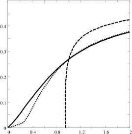
Figure 1: Occupation of the excited level as a function of $\alpha T$, for $\rho=1$, $\beta_{0}E_{1}=1$, and $\alpha=0.5$ (solid line), resp. $1.0$ (dotted), and $2.0$ (dashed).

5.4 Why nonlinear averages?

We now show how nonlinear averages arise in a natural way.

Note that

$$\phi_{\alpha}(\beta_{0}(E-U)/N) = \frac{e^{(1-\alpha)\beta_{0}(E_{\sigma}-U)/N}-1}{1-\alpha}$$ (116)

$$= \frac{e^{(1-\alpha)\beta_{0}E/N}-e^{(1-\alpha)\beta_{0}U/N}}{(1-\alpha)e^{(1-\alpha)\beta_{0}U/N}}$$ (117)

$$= \frac{1}{N}\,\frac{\phi_{\alpha_{N}}(\beta_{0}E)-\phi_{\alpha_{N}}(\beta_{0}U)}{\phi^{\prime}_{\alpha_{N}}(\beta_{0}U)}$$ (118)

with $1-\alpha_{N}=(1-\alpha)/N$. In particular, the equation $\phi_{\alpha}(\beta_{0}(E-U)/N)\approx\epsilon$ appearing in the l.h.s. of (59), can be rewritten as

$$\phi_{\alpha_{N}}(\beta_{0}E)-\phi_{\alpha_{N}}(\beta_{0}U)\approx\phi^{\prime}_{\alpha_{N}}(\beta_{0}U)\,\epsilon.$$ (119)

This implies that (59) can be written as

$$\hbox{Prob}\left((\phi_{\alpha_{N}}(\beta_{0}E)-\phi_{\alpha_{N}}(\beta_{0}U))/N\approx\epsilon\right)\sim\exp(-Nr_{*}(\epsilon))$$ (120)

with

$$r_{*}(\epsilon)=r\circ\phi_{\alpha}^{-1}\left(\epsilon/\phi^{\prime}_{\alpha}(\beta_{0}U/N)\right)$$ (121)

The problem is now to find a probability distribution $p_{\sigma}$ for which (120) is satisfied. A candidate solution to this problem is obtained by maximizing entropy with the constraint that

$$\sum_{\sigma}p_{\sigma}\phi_{\alpha_{N}}(\beta_{0}E_{\sigma})=\phi_{\alpha_{N}}(\beta_{0}U)$$ (122)

The latter condition can be written as

$$\langle\beta_{0}E\rangle=\beta_{0}U$$ (123)

with average $\langle\cdot\rangle$ calculated as a KN-mean w.r.t. the function $\phi_{\alpha_{N}}$. This justifies the use of nonlinear KN-averages.

Remains the question which entropy should be optimized. We believe that in many applications the right choice is either Shannon’s entropy or an $\alpha$-entropy of Rényi (or an equivalent entropy like that of Tsallis). The reason for this belief is that these are the only entropies with nice additivity properties.

5.5 Rényi thermostatistics of the Curie-Weiss model

We reconsider the Curie-Weiss model, now with the function $\phi$ equal to $\phi_{\alpha,1}\equiv\phi_{\alpha}$. It is not the intention here to treat this model in detail, with arbitrary values of $\alpha$ and $\rho$. We rather want to to discuss the thermodynamic limit in the extensive $\rho=1$-case.

Introduce the notations $m=M/N$ and $u=U/N$, and

$$\gamma(m)=\exp((1-\alpha)\beta_{0}(Jm^{2}/2+hm+u)).$$ (124)

The equilibrium probabilities are, assuming $0<\alpha<1$, (see (49) and the discussion of the previous subsection)

$$p(M) = {N\choose\frac{N+M}{2}}\frac{1}{Z}\left[\alpha_{N}+(1-\alpha_{N})\frac{\phi_{\alpha_{N}}(\beta_{0}E_{\sigma})-\phi_{\alpha_{N}}(\beta_{0}U)}{\phi^{\prime}_{\alpha_{N}}(\beta_{0}U)\beta_{0}T}\right]^{1/(\alpha_{N}-1)}$$ (125)

$$= {N\choose\frac{N+M}{2}}\frac{1}{Z}\left[\alpha_{N}-\frac{1}{\beta_{0}T}\left(1-\frac{1}{\gamma(m)}\right)\right]^{-N/(1-\alpha)}$$ (126)

$$\sim \exp\bigg{[}-Ns(m)\bigg{]},$$ (127)

with

$$s(m) = s_{\infty}(m)+\frac{1}{1-\alpha}\ln\left[1-\frac{1}{\beta_{0}T}\left(1-\frac{1}{\gamma(m)}\right)\right]$$ (128)

(assuming $T>J$). The first derivative of $s(m)$ is

$$I^{\prime}(m) = \frac{1}{2}\ln\frac{1+m}{1-m}-\frac{\beta_{0}(Jm+h)}{1+(\beta_{0}T-1)\gamma(m)}$$ (129)

Let $m_{*}$ be the value of $m$ for which $s(m)$ is maximal. It is a solution of $I^{\prime}(m)=0$. Hence it satisfies

$$m_{*}=\tanh\left(\frac{\beta_{0}(Jm_{*}+h)}{1+(\beta_{0}T-1)\gamma(m_{*})}\right)$$ (130)

But $\gamma(m_{*})=1+\hbox{O}(1/N)$ holds for large $N$, so that the previous equation simplifies to the standard mean-field equation (70).

In case $T>J$ the rate function $s(m)$ does not differ significantly from the standard result $s_{\infty}(m)-Jm^{2}/2T$. If $T<J$ the difference consists in the first place of a constant term. All together, the present treatment of the Curie-Weiss model seems to yield results which are very similar to the standard one.

6 Discussion

We have presented a formalism of thermostatistics based on Kolmogorov-Nagumo averages and Hartley’s information measure. It treats the problem of maximizing average information $\langle I\rangle$ under the constraint that average energy $\langle\beta_{0}E\rangle$ has some given value $\beta_{0}U$. The KN-average $\langle\cdot\rangle$ is determined by a monotonic function $\phi$ and by probabilities $p_{k}$. The same KN-average is used to define average energy and to define entropy as an average information content. In the present paper the function $\phi$ is kept constant while the probabilities $p_{k}$ are varied. It could be interesting to consider cases where $\phi$ is varied as well.

Of particular interest is the case when $\phi$ is an exponential function because then the average information $\langle I\rangle$ coincides with Rényi’s entropy. As proved by Rényi, his $\alpha$-entropies, together with that of Shannon, are the only additive ones. Instead of exponential $\phi$ we use a slightly modified function (21), for which $\langle I\rangle$ is still Rényi’s entropy. We call the statistical formalism obtained in this way Rényi thermostatistics. It generalizes the standard formalism of Boltzmann-Gibbs. Note that Rényi thermostatistics is extensive in the sense that, when a system is composed of independent subsystems and the probabilities are of the product form, then both average information and average energy of the total system are the sum of the corresponding subsystem averages. From the examples of the Curie-Weis model (section 5.5) and the two-level model (section 5.3) it seems that Rényi thermostatistics behaves quite similar to the standard formalism. The most striking difference is the energy cut-off which can occur in case $\alpha>1$. When this happens then the probability of occupation of high-energy levels is exactly zero. In particular, this kind of equilibrium state is not a Gibbs measure.

We have tried to justify the use of KN-averages in statistical mechanics. In essence, a KN-average consists of a change of scale by means of a function $\phi$, followed by a statistical average using probabilities $p_{k}$, and a final back transformation using the inverse function $\phi^{-1}$. A basic ingredient of statistical mechanics is the equivalence of ensembles. A possible reason for combining the canonical ensemble with a change of scale is that in this way the equivalence of ensembles might be restored. We did not consider equivalence of ensembles directly, but argued on the level of fluctuations of energy. These should be exponentially small in order to apply the theory of large deviations. It is intuitively clear that a change of scale influences the scale of fluctuations. This is indeed confirmed by calculations on the Curie-Weiss model which we used as an example. Now, if the function $\phi$ is the function involved in the definition of Rényi’s entropy, then scaled energy fluctuations can be expressed as fluctuations of the scaled energy. In this way we can justify that scaled energy is the relevant quantity of the canonical ensemble.

In a natural way Tsallis’ entropy appears as a tool for calculating equilibrium averages in Rényi thermostatistics. This offers the opportunity to reuse knowledge from Tsallis-like thermostatistics. It shines also new light onto Tsallis’ nonextensive thermostatistics because there is a one-to-one translation of problems from the one formalism to the other. There are many applications of the Tsallis formalism — see e.g. the review paper [26]. An open question is how many of these applications have a natural formulation in terms of Rényi thermostatistics. As a first guess this would be the case whenever extensivity is important.

We consider also a further generalization of extensive Rényi thermostatistics to a non-extensive formalism. This extended formalism includes, besides the extensive case, also nonextensive Tsallis thermostatistics. In particular, an argument has been presented which settles the problem of defining thermodynamic temperature in a nonextensive context.

A short version of the present paper has appeared in [33].

Acknowledgements

One of the authors (MC) wishes to thank the NATO for a research fellowship enabling his stay at the Universiteit Antwerpen.

Appendix

Definition (15) of the $\alpha$-deformed logarithm $\ln_{\alpha}(x)$, without the condition $x\geq 1$, is what is found in literature [18, 25]. The inverse function $\exp_{\alpha}(x)$ is not defined for all $x$, while we need it for all $x$ in section 5. Therefore we propose the following extended definition

$$\ln_{\alpha}(x) = \frac{x^{1-\alpha}-1}{1-\alpha}\qquad\hbox{ if }x\geq 1$$ (131)

$$= \frac{x^{\alpha-1}-1}{\alpha-1}\qquad\hbox{ if }0<x\leq 1$$ (132)

(we assume $\alpha>0$, $\alpha\not=1$). It satisfies $\ln_{\alpha}(1)=0$. The deformed logarithm $\ln_{\alpha}(x)$ converges in the limit $\alpha=1$ to the natural logarithm $\ln(x)$.

The derivative of $\ln_{\alpha}(x)$ is a continuous positive function given by

$$\frac{{\rm d}\,}{{\rm d}x}\ln_{\alpha}(x) = x^{-\alpha}\qquad\hbox{ if }x\geq 1$$ (133)

$$= x^{\alpha-2}\qquad\hbox{ if }0<x\leq 1$$ (134)

In particular, this implies that $\ln_{\alpha}(x)$ is a strictly increasing function of $x$. Note that

$$-\frac{1}{\alpha-1}<\ln_{\alpha}(x)<\frac{1}{\alpha-1}\qquad\hbox{ if }\alpha>1$$ (135)

while for $0<\alpha<1$ the deformed logarithm takes on any real value. Hence, the inverse function $\exp_{\alpha}(x)$ has a limited domain of definition in the former case. One finds

$$\exp_{\alpha}(x) = \left[1+(1-\alpha)x\right]_{+}^{1/(1-\alpha)}\qquad\hbox{ if }x\geq 0$$ (136)

$$= \left[1+(\alpha-1)x\right]_{+}^{1/(\alpha-1)}\qquad\hbox{ if }x\leq 0$$ (137)

Clearly, $\exp_{\alpha}(0)=1$ and $\exp_{\alpha}(x)$ cannot be negative. In the limit $\alpha=1$ the deformed exponential function $\exp_{\alpha}(x)$ converges to the usual exponential function $\exp(x)$.

The derivative of $\exp_{\alpha}(x)$

$$\frac{{\rm d}\,}{{\rm d}x}\exp_{\alpha}(x) = \left(\exp_{\alpha}(x)\right)^{\alpha}\qquad\hbox{ if }x\geq 0$$ (138)

$$= \left(\exp_{\alpha}(x)\right)^{2-\alpha}\qquad\hbox{ if }x\leq 0$$ (139)

is a positive continuous function. In particular, this implies that $\exp_{\alpha}(x)$ is a strictly increasing function on its domain of definiton.

Finally, note that

$$\exp_{\alpha}(-x)=1/\exp_{\alpha}(x)\qquad\hbox{ and }\quad\ln_{\alpha}(1/x)=-\ln_{\alpha}(x).$$ (140)

References

- [1]
- [2] R.V. Hartley, Transmission of information, Bell System Technical Journal, 7, 1928.
- [3] A. Kolmogorov, Atti della R. Accademia Nazionale dei Lincei 12, 388 (1930).
- [4] M. Nagumo, Japan. J. Math. 7, 71 (1930).
- [5] C.E. Shannon, Bell System Technical J. 27, 379 (1948); 27, 623 (1948).
- [6] E.T. Jaynes,Information theory and statistical mechanics. Part I. Phys. Rev. 106, 620-630 (1957); Part II. Phys. Rev.108, 171-191 (1957).
- [7] J. Harvda, F. Charvat, Kybernetica 3, 30 (1967).
- [8] Z. Daróczy, Inf. Control, 16, 36- (1970).
- [9] A. Rényi, Some Fundamental Questions of Information Theory. Selected Papers of Alfred Renyi, Vol 2, (Akademia Kiado, Budapest, 1976) pp 526-552.
- [10] A. Rényi, On Measures of Entropy and Information. Selected Papers of Alfred Rényi, Vol. 2. (Akademia Kiado, Budapest, 1976) pp 565-580.
- [11] A. Wehrl, General properties of entropy, Rev. Mod. Phys. 50, 221-260 (1978).
- [12] R.S. Ellis, Entropy, large deviations, and statistical mechanics (Springer-Verlag, New York, 1985)
- [13] C. Tsallis, Possible Generalization of Boltzmann-Gibbs Statistics, J. Stat. Phys. 52, 479-487 (1988).
- [14] R.S. Ellis, K. Wang, Limit theorems for the empirical vector of the Curie-Weiss-Potts model, Stoch. Proc. Appl. 35, 59-79 (1990).
- [15] R.M. Gray, Entropy and information theory (Springer Verlag, 1990)
- [16] E.M.F. Curado and C. Tsallis, Generalized statistical mechanics: connection with thermodynamics, J. Phys. A24, L69-L72 (1991).
- [17] A.R. Plastino, A. Plastino, Stellar polytropes and Tsallis’ entropy, Phys. Lett. A174, 384-386 (1993).
- [18] C. Tsallis, What are the numbers that experiments provide?, Quimica Nova 17(6), 468-471 (1994).
- [19] J.T. Lewis, C.-E. Pfister, W.G. Sullivan, Large deviations and the thermodynamic formalism: a new proof of the equivalence of ensembles, in: On three levels, ed. M. Fannes, C. Maes, A. Verbeure (Plenum press, New York, 1994)
- [20] J.T. Lewis, C.-E. Pfister, W.G. Sullivan, The equivalence of ensembles for lattice systems: some examples and a counterexample, J. Stat. Phys. 77(1/2), 397-419 (1994).
- [21] J.T. Lewis and C.-E. Pfister, Thermodynamic probability theory: some aspects of large deviations, Russian Math. Surveys, 50(2), 279-317 (1995).
- [22] N. Meyer-Vernet, M. Moncuquet, and S. Hoang, Temperature inversion in the Io plasma torus, Icarus 116, 202-213 (1995).
- [23] L.S. Lucena, L.R. da Silva, C. Tsallis, Departure from Boltzmann-Gibbs statistics makes the hydrogen-atom specific heat a computable quantity, Phys. Rev. E51, 6247-6249 (1995)
- [24] C. Tsallis, R.S. Mendes, A.R. Plastino, The role of constraints within generalized nonextensive statistics, Physica A261, 543-554 (1998).
- [25] E.P. Borges, On a -generalization of circular and hyperbolic functions, J. Phys. A 31, 5281-5288 (1998).
- [26] C. Tsallis, Nonextensive statistics: theoretical, experimental and computational evidences and connections, Braz. J. Phys. 29(1), 1-35 (1999).
- [27] J. Naudts, Rigorous results in non-extensive thermodynamics, math-ph/9908025, Rev. Math. Phys., 12(10), 1305-1324 (2000).
- [28] A. V. Milovanov and L. M. Zelenyi, Functional background of the Tsallis entropy: ”coarse-grained” systems and ”kappa” distribution functions, Nonlinear Processes in Geophysics, 7(3/4), 211-221 2000.
- [29] J. Naudts and M. Czachor, Dynamic and thermodynamic stability of non-extensive systems, in: ”Nonextensive Statistical Mechanics and Its Applications”, ed. S. Abe, Y. Okamoto, Lecture Notes in Physics 560 (Springer-Verlag, 2001), p. 243-252.
- [30] S. Abe, A. Martinez, F. Pennini, A. Plastino, Nonextensive thermodynamics relations, Phys. Lett. A281(2-3), 126-130 (2001).
- [31] J. Naudts, Dual description of nonextensive ensembles, in: ”Classical and Quantum Complexity and Nonextensive Thermodynamics”, eds. C. Tsallis, P. Grigolini, and B. West, Chaos, Solitons, and Fractals 13(3),445-450 (2002).
- [32] R. Toral, On the definition of physical temperature and pressure for nonextensive thermostatistics, June 2001, cond-mat/0106060.
- [33] J. Naudts and M. Czachor, Thermostatistics based on Kolmogorov-Nagumo averages: Unifying framework for extensive and nonextensive generalizations cond-mat/0106324.
- [34] E. Vives and A Planes, Intensive variables and fluctuations in non-extensive thermodynamics: the generalized Gibbs-Duhem equation and Einstein’s formula, cond-mat/0106428.