Grassmannian Fields and Doubly Enhanced Skyrmions
in Bilayer Quantum Hall system at $\nu=2$

Abstract

At the filling factor $\nu=2$ the bilayer quantum Hall system has three phases, the ferromagnetic phase (spin phase), the spin singlet phase (ppin phase) and the canted antiferromagnetic phase. We analyze soft waves and quasiparticle excitations in the spin and ppin phases. It is shown that the dynamic field is the Grassmannian G_4,2 field carrying four complex degrees of freedom. In each phase there are four complex soft waves (pseudo-Goldstone modes) and one kind of skyrmion excitations (G_4,2 skyrmions) flipping either spins or pseudospins coherently. An intriguing property is that a quasiparticle is a G_4,2 skyrmion essentially consisting of two CP³ skyrmions and thus possesses charge $2e$.

I Introduction

Quantum Hall (QH) effects have attracted renewed attentionBookDasSarma ; BookEzawa owing to its peculiar features associated with quantum coherence. SkyrmionsSondhi93B are charged excitations reversing several electron spins coherently, whose existence has been established firmly in monolayer QH systemsBarrett95L ; Aifer96L ; Schmeller95L . Bilayer quantum Hall (BLQH) systems are much more interesting because they exhibit unique QH effects originating in the interlayer interaction. For instance, we may have not only skyrmions in the spin space but also skyrmions in the layer (pseudospin) spaceEzawa97B ; Ezawa99L . Furthermore, an anomalous tunneling current has been observedSpielman00L between the two layers at the zero bias voltage. It may well be a manifestation of the Josephson-like phenomena predicted a decade agoEzawa92IJMPB . They occur due to quantum coherence developed spontaneously across the layersEzawa97B ; Moon95B .

Electrons make cyclotron motions and their energies are quantized into Landau levels under perpendicular magnetic field $B_{\perp}$. The number density of magnetic flux quanta is $\rho_{\Phi}\equiv B_{\perp}/\Phi_{\text{D}}$, where $\Phi_{\text{D}}=2\pi\hbar/e$ is the flux unit. One electron occupies an area $2\pi\ell_{B}^{2}$ with $\ell_{B}=\sqrt{\hbar/eB_{\perp}}$ the magnetic length. The filling factor is $\nu=\rho_{0}/\rho_{\Phi}$ with $\rho_{0}$ the electron number density. In the BLQH system one Landau site may accommodate four isospin states $|\text{f}\!\uparrow\rangle$, $|\text{f}\!\downarrow\rangle$, $|\text{b}\!\!\uparrow\rangle$, $|\text{b}\!\!\downarrow\rangle$ in the lowest Landau level (LLL), where $|\text{f}\!\uparrow\rangle$ implies that the electron is in the front layer and its spin is up and so on. The SU(4) symmetry underlies the BLQH system provided the cyclotron energy is large enough.

The driving force of quantum coherence is the Coulomb exchange interaction. It is described by an anisotropic SU(4) nonlinear sigma model in BLQH systems, as is most easily demonstrated in the von-Neumann-lattice formulationEzawaX02B . The BLQH system at $\nu=1$ has been extensively analyzedEzawaX02B ; RJ based on this SU(4) scheme, where the dynamic field is the CP³ field carrying three complex degrees of freedom. It has been shown at $\nu=1$ that there are three complex soft waves (pseudo-Goldstone modes) and one kind of skyrmion excitations (CP³ skyrmions) flipping both spins and pseudospins coherently.

New features appear in the BLQH system at $\nu=2$, where two distinguishable phases have clearly been observed experimentallyPelle97 ; Sawada98L ; Sawada99R . One is a fully spin polarized ferromagnetic phase, which we call the spin phase. The other is a spin singlet phase, which we call the pseudospin (abridged as ppin) phase because it is also a fully pseudospin polarized one. (The layer degree of freedom is referred to as the pseudospin.) It has been argued that there arises a new phase, called canted antiferromagnetic phaseDemler99L ; Zheng97L ; Sarma97L , between the spin and ppin phases in the phase diagram. It is realized by the effect of the SU(4)-noninvariant part of the Coulomb exchange interaction. However, according to an exact numerical diagonalization method on few-electron systemsSchliemann00L the canted phase occupies a very tiny region in the phase diagram and is practically negligible, as is consistent with experimental resultsPelle97 ; Sawada98L ; Sawada99R .

The aim of this paper is to analyze soft waves and topological solitons in the spin and ppin phases. The Hilbert space in the lowest Landau level is spanned by the six states occupying two of the four isospin states. An intriguing property is that one quasiparticle consists of two skyrmions and thus possesses charge $2e$, as was pointed out in Ref.BookEzawa ; Ezawa99L . However, the previous analysis is primitive and incomplete. We present a theory of the $\nu=2$ BLQH system based on the SU(4) scheme with the Grassmannian manifold. We show that the dynamic field is the Grassmannian G_4,2 field carrying four complex degrees of freedom and that the Coulomb exchange interaction is described by the Grassmannian G_4,2 sigma model. In each phase there are four complex soft waves (pseudo-Goldstone modes) and one kind of skyrmion excitations (G_4,2 skyrmions) flipping either spins or pseudospins coherently. We confirm that one G_4,2 skyrmion essentially consists of two CP³ skyrmions and carries charge $2e$.

In section II, after reviewing the microscopic Landau-site HamiltonianEzawaX02B for the BLQH system, we present an improved expression for the Coulomb exchange interaction. In section III we make a group theoretical study of isospin states in the BLQH system. At $\nu=2$ they belong to the $\boldsymbol{6}$-dimensional representation of SU(4). Classifying them with respect to the subgroup SU${}_{\text{spin}}$(2)$\otimes$SU${}_{\text{ppin}}$(2), we introduce the spin phase and the ppin phase. In section IV, we investigate the SU(4) invariant limit of the $\nu=2$ BLQH system, where the symmetry SU(4) is spontaneously broken into U(1)$\otimes$SU(2)$\otimes$SU(2). There are eight broken generators; $S_{x}$, $S_{y}$, $2S_{x}P_{a}$ and $2S_{y}P_{a}$ in the spin phase, and $P_{y}$, $P_{z}$, $2S_{a}P_{y}$ and $2S_{a}P_{z}$ in the ppin phase, where $S_{a}$ and $P_{a}$ are respectively the generators of the groups SU${}_{\text{spin}}$(2) and SU${}_{\text{ppin}}$(2). Accordingly there arise eight Goldstone modes in the SU(4) invariant limit. The target space becomes the Grassmannian G_4,2 manifold, whose real dimension is eight. In section V, we introduce the composite-boson (CB) picture of electrons to make a further study of the Goldstone modes. The CP³ field is defined as the normalized CB field. To describe two electrons in one Landau site we introduce two CP³ fields. By requiring that two electrons are indistinguishable, the set of two CP³ fields turns out to be the Grassmannian G_4,2 field $Z(\boldsymbol{x})$. It is a $4\times 2$ matrix field carrying eight real independent components representing the Goldstone modes. In section VI, we construct the Hamiltonian in the $\boldsymbol{6}$-dimensional representation of SU(4), where the basic field is the Grassmannian field $Z(\boldsymbol{x})$. We analyze the soft modes which are the pseudo-Goldstone modes made gapful by the Zeeman or tunneling gap. In section VII we analyze topological solitons (G_4,2 skyrmions), whose existence follows from the homotopy theorem, $\pi_{2}($G${}_{4,2})=\mathbb{Z}$, with $\mathbb{Z}$ the integer additive group. Analyzing the condition that they are confined within the lowest Landau level, we find that they are comprised of two skyrmions excited in the front and back layers for the spin phase, or in the up-spin and down-spin states for the ppin phase. We call them biskyrmions. In section VIII, we present an effective spin-1 theory of biskyrmions. It is shown that they are represented as the well-known O(3) skyrmions in this effective spin-1 theory. In section IX we study the criterion whether the system is to be regarded as a genuine BLQH system with biskyrmion excitations or as a set of two monolayer QH systems with simple skyrmion excitations. Recent experimental dataKumada00L have revealed a remarkable difference in the activation energy behavior between two bilayer samples with small and large tunneling gaps. We explain it based on this criterion.

II Exchange Interactions

The kinetic Hamiltonian of planar electrons in the bilayer system is given by

$$H_{\text{K}}={\frac{1}{2M}}\int d^{2}x\boldsymbol{\psi}^{\dagger}(\boldsymbol{x})(D_{x}-iD_{y})(D_{x}+iD_{y})\boldsymbol{\psi}(\boldsymbol{x})$$ (1)

apart from the cyclotron energy $N\hbar\omega_{\text{c}}/2$, where $D_{k}=-i\hbar\partial_{k}+eA_{k}$. The electron field $\boldsymbol{\psi}$ possesses the SU(4) isospin index $\sigma=\text{f}\!\uparrow,\text{f}\!\downarrow,\text{b}\!\uparrow,\text{b}\!\downarrow$. When the cyclotron gap is large enough, thermal excitations across Landau levels are practically impossible. Hence, it is a good approximation to neglect all those excitations by requiring the confinement of electrons to the lowest Landau level. This leads to the LLL condition on the state,

$$(D_{x}+iD_{y})\psi^{\sigma}(\boldsymbol{x})|\varphi\rangle=0,$$ (2)

implying that the kinetic energy (1) vanishes. It determines the Hilbert space $\mathbb{H}_{\text{LLL}}$.

We analyze electrons confined to the lowest Landau level. One Landau site contains four electron states distinguished by the SU(4) isospin index $\sigma$. The group SU(4) is generated by the Hermitian, traceless, $4\times 4$ matrices. There are $(4^{2}-1)$ independent matrices. We take a standard basisBookGeorgi , $\lambda_{a}$, $a=1,2,\cdots,15$, normalized as $\text{Tr}(\lambda_{a}\lambda_{b})=2\delta_{ab}$. They are the generalization of the Pauli matrices.

The Coulomb interaction is given by

$$H_{C}=\sum_{\alpha,\beta=\text{f},\text{b}}{\frac{1}{2}}\int d^{2}xd^{2}yV_{\alpha\beta}(\boldsymbol{x}-\boldsymbol{y})\rho_{\alpha}(\boldsymbol{x})\rho_{\beta}(\boldsymbol{y}),$$ (3)

where $V_{\text{f}\text{f}}=V_{\text{b}\text{b}}={e^{2}}/4\pi\varepsilon r$ is the intralayer Coulomb interaction, while $V_{\text{f}\text{b}}=V_{\text{b}\text{f}}={e^{2}}/4\pi\varepsilon\sqrt{r^{2}+d^{2}}$ is the interlayer Coulomb interaction with $d$ the interlayer separation. The Coulomb interaction is decomposed into two terms, $H_{C}=H_{C}^{+}+H_{C}^{-}$, with

$$H_{C}^{+} ={\frac{1}{2}}\int d^{2}xd^{2}yV_{+}(\boldsymbol{x}-\boldsymbol{y})\rho(\boldsymbol{x})\rho(\boldsymbol{y}),$$ (4a)

$$H_{C}^{-} ={\frac{1}{2}}\int d^{2}xd^{2}yV_{-}(\boldsymbol{x}-\boldsymbol{y})\Delta\rho(\boldsymbol{x})\Delta\rho(\boldsymbol{y}),$$ (4b)

where $$V_{\pm}={\frac{1}{2}}(V_{\text{f}\text{f}}\pm V_{\text{f}\text{b}}) H_{C}^{+} \rho(\boldsymbol{x}) H_{C}^{-} \Delta\rho(\boldsymbol{x})$$; depends on the total density , while on the density difference between the front and back layers,

$$\Delta\rho(\boldsymbol{x})=\rho^{\text{f}\uparrow}(\boldsymbol{x})+\rho^{\text{f}\downarrow}(\boldsymbol{x})-\rho^{\text{b}\uparrow}(\boldsymbol{x})-\rho^{\text{b}\downarrow}(\boldsymbol{x}).$$ (5)

The Coulomb term $H_{C}^{+}$, which is invariant under the SU(4) transformation, dominates the BLQH system provided the interlayer separation $d$ is small enough.

The Coulomb exchange interaction is the key to quantum coherence. An easiest way for its derivation is to expand the electron field $\psi^{\sigma}(\boldsymbol{x})$ as

$$\psi^{\sigma}(\boldsymbol{x})=\sum_{i=1}^{N_{\Phi}}c_{\sigma}(i)\varphi_{i}(\boldsymbol{x}),$$ (6)

where $N_{\Phi}$ is the total number of Landau sites; $c_{\sigma}(i)$ is the annihilation operator of the electron with isospin $\sigma$ at Landau site $i$,

$$\{c_{\sigma}(i),c_{\tau}^{\dagger}(j)\} =\delta_{ij}\delta_{\sigma\tau},$$

$$\{c_{\sigma}(i),c_{\tau}(j)\} =\{c_{\sigma}^{\dagger}(i),c_{\tau}^{\dagger}(j)\}=0,$$ (7)

and $\varphi_{i}(\boldsymbol{x})$ is the one body wave function determined to satisfy the LLL condition (2). It describe an electron localized around the Landau site $i$.

We substitute the expansion (6) into the Coulomb interaction terms (4a) and (4b). From the SU(4)-invariant term (4a), we obtain a Landau-site HamiltonianEzawaX02B representing the SU(4)-invariant exchange interaction,

$$H_{X}^{+}=-4\sum_{\langle i,j\rangle}J_{ij}^{+}\biggl{(}\boldsymbol{T}(i)\!\cdot\!\boldsymbol{T}(j)+{\frac{1}{8}}n(i)n(j)\biggr{)}.$$ (8)

Here, the sum $\sum_{\langle i,j\rangle}$ runs over spin pairs just once;$\ \boldsymbol{T}=(T_{1},T_{2},\ldots,T_{15})$ is the SU(4) isospin,

$$T_{a}=(c_{\text{f}\uparrow}^{\dagger},c_{\text{f}\downarrow}^{\dagger},c_{\text{b}\uparrow}^{\dagger},c_{\text{b}\downarrow}^{\dagger}){\frac{\lambda_{a}}{2}}\begin{pmatrix}c_{\text{f}\uparrow}\\ c_{\text{f}\downarrow}\\ c_{\text{b}\uparrow}\\ c_{\text{b}\downarrow}\end{pmatrix},$$ (9)

and $n(i)$ is the electron number operator, $n\equiv\sum_{\sigma}c_{\sigma}^{\dagger}c_{\sigma}$, at each site $i$. The exchange integral $J_{ij}^{\pm}$ is given by

$$J_{ij}^{\pm}={\frac{1}{2}}\int\!d^{2}xd^{2}y\;\varphi_{i}^{\ast}(\boldsymbol{x})\varphi_{j}^{\ast}(\boldsymbol{y})V_{\pm}(\boldsymbol{x}-\boldsymbol{y})\varphi_{i}(\boldsymbol{y})\varphi_{j}(\boldsymbol{x}).$$ (10)

It is notable that the exchange term (8) is rewritten as

$$H_{X}^{+}=-8\sum_{\langle i,j\rangle} J_{ij}^{+}\bigl{(}\boldsymbol{S}(i)\!\cdot\!\boldsymbol{S}(j)+{\frac{1}{4}}n(i)n(j)\bigr{)}$$

$$\check{\otimes}\bigl{(}\boldsymbol{P}(i)\!\cdot\!\boldsymbol{P}(j)+{\frac{1}{4}}n(i)n(j)\bigr{)},$$ (11)

where $\boldsymbol{S}=\boldsymbol{S}^{\text{f}}+\boldsymbol{S}^{\text{b}}$ and $\boldsymbol{P}=\boldsymbol{P}^{\uparrow}+\boldsymbol{P}^{\downarrow}$. The symbol $\check{\otimes}$ is understood as the direct product with respect to the Pauli matrices such as

$$S_{a}P_{b}\equiv S_{a}\check{\otimes}P_{b}=(c_{\text{f}\uparrow}^{\dagger},c_{\text{f}\downarrow}^{\dagger},c_{\text{b}\uparrow}^{\dagger},c_{\text{b}\downarrow}^{\dagger}){\frac{\tau_{a}}{2}}\otimes{\frac{\tau_{b}}{2}}\begin{pmatrix}c_{\text{f}\uparrow}\\ c_{\text{f}\downarrow}\\ c_{\text{b}\uparrow}\\ c_{\text{b}\downarrow}\end{pmatrix}.$$ (12)

Various SU(2) operators are given by

$$S_{a}^{\text{f}} =(c_{\text{f}\uparrow}^{\dagger},c_{\text{f}\downarrow}^{\dagger}){\frac{\tau_{a}}{2}}\begin{pmatrix}c_{\text{f}\uparrow}\\ c_{\text{f}\downarrow}\end{pmatrix}, \;S_{a}^{\text{b}} =(c_{\text{b}\uparrow}^{\dagger},c_{\text{b}\downarrow}^{\dagger}){\frac{\tau_{a}}{2}}\begin{pmatrix}c_{\text{b}\uparrow}\\ c_{\text{b}\downarrow}\end{pmatrix},$$

$$P_{a}^{\uparrow} =(c_{\text{f}\uparrow}^{\dagger},c_{\text{b}\uparrow}^{\dagger}){\frac{\tau_{a}}{2}}\begin{pmatrix}c_{\text{f}\uparrow}\\ c_{\text{b}\uparrow}\end{pmatrix}, \;P_{a}^{\downarrow} =(c_{\text{f}\downarrow}^{\dagger},c_{\text{b}\downarrow}^{\dagger}){\frac{\tau_{a}}{2}}\begin{pmatrix}c_{\text{f}\downarrow}\\ c_{\text{b}\downarrow}\end{pmatrix}.$$ (13)

The equivalence between the Hamiltonians (8) and (11) is seen by expanding the latter as

$$H_{X}^{+}=- 2\sum_{\langle i,j\rangle}J_{ij}^{+}\biggl{(}\boldsymbol{S}(i)\!\cdot\!\boldsymbol{S}(j)+\boldsymbol{P}(i)\!\cdot\!\boldsymbol{P}(j)$$

$$+4S_{a}P_{b}(i)\!\cdot\!S_{a}P_{b}(j)+{\frac{1}{4}}n(i)n(j)\biggr{)}.$$ (14)

We may take $S_{a}$, $P_{a}$, $2S_{a}P_{b}$ instead of $T_{a}$ as the fifteen generators of the group SU(4). These are related by

$$S_{x}=T_{1}+T_{13},\quad S_{y}=T_{2}+T_{14},$$

$$\qquad S_{z}=T_{3}-(1/\sqrt{3})T_{8}+(\sqrt{6}/3)T_{15},$$

$$P_{x}=T_{4}+T_{11},\quad P_{y}=T_{5}+T_{12},$$

$$\qquad P_{z}=(2/\sqrt{3})T_{8}+(2/\sqrt{6})T_{15},$$

$$2S_{x}P_{x}=T_{6}+T_{9},\quad 2S_{x}P_{y}=T_{7}+T_{10},$$

$$\qquad 2S_{x}P_{z}=T_{1}-T_{13},$$

$$2S_{y}P_{x}=-T_{7}+T_{10},\quad 2S_{y}P_{y}=T_{6}-T_{9},$$

$$\qquad 2S_{y}P_{z}=T_{2}-T_{14},$$

$$2S_{z}P_{x}=T_{4}-T_{11},\quad 2S_{z}P_{y}=T_{5}-T_{12},$$

$$\qquad 2S_{z}P_{z}=T_{3}+(1/\sqrt{3})T_{8}-(\sqrt{6}/3)T_{15}.$$ (15)

Note that $2\boldsymbol{T}^{2}=\boldsymbol{S}^{2}+\boldsymbol{P}^{2}+(2S_{a}P_{b})^{2}$.

The exchange energy due to the SU(4)-noninvariant term (4b) is also evaluated. Combining them we obtain

$$H_{X}= -8\sum_{\langle i,j\rangle}J_{ij}\biggl{(}\boldsymbol{S}(i)\!\cdot\!\boldsymbol{S}(j)+\frac{1}{4}n(i)n(j)\biggr{)}$$

$$\check{\otimes}\biggl{(}\sum_{a}^{x,y,z}\frac{J_{ij}^{a}}{J_{ij}}P_{a}(i)P_{a}(j)+\frac{1}{4}n(i)n(j)\biggr{)},$$ (16)

where $J_{ij}^{x}=J_{ij}^{y}=J_{ij}^{d}\equiv J_{ij}^{+}-J_{ij}^{-}$ and $J_{ij}^{z}=J_{ij}\equiv J_{ij}^{+}+J_{ij}^{-}$. The exchange term represents interactions between isospins in two sites due to the overlapping of their wave functions. For instance, the term $\boldsymbol{S}\!\cdot\!\boldsymbol{S}$ contains

$$\bigl{\{}\boldsymbol{S}(i)\!\cdot\!\boldsymbol{S}(j)\bigr{\}}_{xy}\equiv{\frac{1}{2}}\bigl{(}S_{+}(i)S_{-}(j)+S_{-}(i)S_{+}(j)\bigr{)},$$ (17)

where ${S}_{\pm}=S_{x}\pm iS_{y}$ are the ladder operators. The term (17) has a role to flip the up-spin in $j$-site and the down-spin in $i$-site simultaneously and vise versa. Thus, the exchange term is the origin of isospin modulation.

III Ground States

We classify isospin states at $\nu=2$, where one Landau site contains two electrons. Each electron belongs to the $\boldsymbol{4}$-dimensional irreducible representation of SU(4). A pair of electrons is classified according to the group-theoretical composition rule,

$$\boldsymbol{4}\otimes\boldsymbol{4}=\boldsymbol{1}\boldsymbol{0}\oplus\boldsymbol{6}.$$ (18)

The $\boldsymbol{1}\boldsymbol{0}$-dimensional irreducible representation is a symmetric state, while the $\boldsymbol{6}$-dimensional irreducible representation is an antisymmetric state. Two electrons in one Landau site must form an antisymmetric state due to the Pauli exclusion principle. Hence, the allowed representation is the antisymmetric $\boldsymbol{6}$-dimensional irreducible representation.

In the language of the subgroup SU${}_{\text{spin}}$(2)$\otimes$SU${}_{\text{ppin}}$(2), the $\boldsymbol{6}$-dimensional irreducible representation of the group SU(4) is divided into two different irreducible representations,

$$\boldsymbol{6}=(\boldsymbol{3},\boldsymbol{1})+(\boldsymbol{1},\boldsymbol{3}),$$ (19)

where $\boldsymbol{3}$ is the symmetric representation of SU(2), and $\boldsymbol{1}$ is the antisymmetric representation of SU(2). Consequently, there are six states at each Landau site, which are grouped into two sectors, i.e., the $(\boldsymbol{3},\boldsymbol{1})$ sector and the $(\boldsymbol{1},\boldsymbol{3})$ sector. We call the $(\boldsymbol{3},\boldsymbol{1})$ sector the spin sector and the $(\boldsymbol{1},\boldsymbol{3})$ sector the ppin sector.

The spin sector $(\boldsymbol{3},\boldsymbol{1})$ consists of spin-triplet pseudospin-singlet states [Fig.1(a)],

$$|t_{\uparrow}\rangle=|\text{f}^{\uparrow},\text{b}^{\uparrow}\rangle,\quad\quad|t_{0}\rangle={\frac{1}{\sqrt{2}}}\bigl{(}|\text{f}^{\uparrow},\text{b}^{\downarrow}\rangle+|\text{f}^{\downarrow},\text{b}^{\uparrow}\rangle\bigr{)},$$

$$|t_{\downarrow}\rangle=|\text{f}^{\downarrow},\text{b}^{\downarrow}\rangle,$$ (20)

where $|\text{f}^{\uparrow},\text{b}^{\uparrow}\rangle\equiv c_{\text{f}\uparrow}^{\dagger}c_{\text{b}\uparrow}^{\dagger}|0\rangle$, etc.

The ppin sector $(\boldsymbol{1},\boldsymbol{3})$ consists of spin-singlet pseudospin-triplet states [Fig.1(b)],

$$|\tau_{+}\rangle=|\text{f}^{\uparrow},\text{f}^{\downarrow}\rangle,\quad\quad|\tau_{0}\rangle=\frac{1}{\sqrt{2}}\bigl{(}|\text{f}^{\uparrow},\text{b}^{\downarrow}\rangle-|\text{f}^{\downarrow},\text{b}^{\uparrow}\rangle\bigr{)},$$

$$|\tau_{-}\rangle=|\text{b}^{\uparrow},\text{b}^{\downarrow}\rangle,$$ (21)

where $|\text{f}^{\uparrow},\text{f}^{\downarrow}\rangle\equiv c_{\text{f}\uparrow}^{\dagger}c_{\text{f}\downarrow}^{\dagger}|0\rangle$, etc.

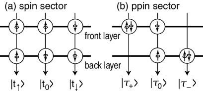
Figure 1: (a) The spin sector is comprised of spin-triplet ppin-singlet states, $|t_{\uparrow}\rangle$, $|t_{0}\rangle$ and $|t_{\downarrow}\rangle$. (b) The ppin sector is comprised of spin-singlet ppin-triplet states, $|\tau_{+}\rangle$, $|\tau_{0}\rangle$ and $|\tau_{-}\rangle$.

In the SU(4)-invariant limit all these six states are degenerate. Actually the degeneracy is resolved by various SU(4)-noninvariant interactions. We write down direct interaction terms to determine the ground state as well as perturbative excitations. Because the QH system is robust against density fluctuations, the direct Coulomb term arising from the SU(4)-invariant term (4a) is irrelevant as far as perturbative fluctuations are concerned. The SU(4)-noninvariant term (4b) yields the capacitance term,

$$H_{\text{cap}}=\varepsilon_{\text{cap}}\sum_{i=1}^{N_{\Phi}}P_{z}(i)P_{z}(i),$$ (22)

where $P_{z}=P_{z}^{\uparrow}+P_{z}^{\downarrow}$ at each site and

$$\varepsilon_{\text{cap}}=\frac{e^{2}}{4\pi\varepsilon\ell_{B}}\sqrt{\frac{\pi}{2}}\biggl{(}1-e^{d^{2}/2\ell_{B}^{2}}\bigl{\{}1-\text{erf}\bigl{(}d/\sqrt{2}\ell_{B})\bigr{\}}\biggr{)}$$ (23)

with the error function $\text{erf}(x)$. The term $\varepsilon_{\text{cap}}P_{z}(i)P_{z}(i)$ represents the capacitance energy per one Landau site. Including the Zeeman and tunneling terms, the direct interaction is summarized as

$$H_{D}=\sum_{i=1}^{N_{\Phi}}\biggl{(}-{\Delta}_{\text{Z}}S_{z}(i)+{{\varepsilon}_{\text{cap}}}P_{z}(i)P_{z}(i)-{\Delta}_{\text{SAS}}P_{x}(i)\biggr{)},$$ (24)

where ${\Delta}_{\text{Z}}$ and ${\Delta}_{\text{SAS}}$ are the Zeeman and tunneling gaps.

The total Landau-site Hamiltonian is

$$H_{\text{total}}=H_{X}+H_{D},$$ (25)

which is the sum of the exchange term (16) and the direct term (24).

The ground state and its energy are obtained by diagonalizing the Hamiltonian (25). The Hilbert space consists of six states. Because the spin and ppin sectors belong to different irreducible representations of SU${}_{\text{spin}}$(2)$\otimes$SU${}_{\text{ppin}}$(2), we have $\langle t_{a}|\boldsymbol{S}|\tau_{b}\rangle=0$ and so on. It follows that $\langle t_{a}|H_{D}|\tau_{b}\rangle=0$ for any $a$ and $b$. Therefore, the spin and ppin sectors are decoupled completely as far as the direct interaction is concerned. This is the case also for the SU(4)-invariant part of the Coulomb exchange interaction. These two sectors are mixed only by the SU(4)-noninvariant exchange interaction. The mixing between the spin and ppin sectors is absent in the vanishing limit of the interlayer separation ($d\rightarrow 0$). It is reasonable to start with this limit and then improve approximation. Thus, we diagonalize the Hamiltonian in the spin and ppin sectors to obtain the ground state. The SU(4)-noninvariant part of the Coulomb exchange interaction is included into the ground-state energy by way of its expectation value.

In the spin sector, the energies are given by

$$E_{t_{\uparrow}} =-2J-\Delta_{Z},$$

$$E_{t_{0}} =-2J,$$

$$E_{t_{\downarrow}} =-2J+\Delta_{Z}.$$ (26)

The ground state of the spin sector is $\prod_{i=1}^{N_{\Phi}}|t_{\uparrow}\rangle_{i}$ with the energy $N_{\Phi}E_{t_{\uparrow}}$.

In the ppin sector, the direct interaction reads

$$H_{D}=\sum_{i}^{N_{\Phi}}\begin{pmatrix}\varepsilon_{\text{cap}}&-\frac{1}{\sqrt{2}}{\Delta}_{\text{SAS}}&0\\ -\frac{1}{\sqrt{2}}{\Delta}_{\text{SAS}}&0&\ -\frac{1}{\sqrt{2}}{\Delta}_{\text{SAS}}\\ 0&-\frac{1}{\sqrt{2}}{\Delta}_{\text{SAS}}&\varepsilon_{\text{cap}}\end{pmatrix}_{i}.$$ (27)

At each site the eigenstates are given by

$$|v_{+}\rangle =\frac{\cos\theta-\sin\theta}{2}(|\tau_{+}\rangle+|\tau_{-}\rangle)+\frac{\cos\theta+\sin\theta}{\sqrt{2}}|\tau_{0}\rangle,$$

$$|v_{0}\rangle =\frac{1}{\sqrt{2}}(|\tau_{+}\rangle-|\tau_{-}\rangle),$$

$$|v_{-}\rangle =\frac{\cos\theta+\sin\theta}{2}(|\tau_{+}\rangle+|\tau_{-}\rangle)+\frac{\cos\theta-\sin\theta}{\sqrt{2}}|\tau_{0}\rangle,$$ (28)

where

$$\tan\theta=\frac{\varepsilon_{\text{cap}}}{2{\Delta}_{\text{SAS}}+\sqrt{4{\Delta}_{\text{SAS}}^{2}+\varepsilon_{\text{cap}}^{2}}},$$ (29)

with the eigenenergies

$$E_{v_{+}} =-(J+J^{d}\cos^{2}(2\theta))+{\frac{1}{2}}\bigl{(}\varepsilon_{\text{cap}}-\sqrt{4{\Delta}_{\text{SAS}}^{2}+\varepsilon_{\text{cap}}^{2}}\bigr{)},$$

$$E_{v_{0}} =-(J+J^{d}\cos^{2}(2\theta))+\varepsilon_{\text{cap}},$$

$$E_{v_{-}} =-(J+J^{d}\cos^{2}(2\theta))+{\frac{1}{2}}\bigl{(}\varepsilon_{\text{cap}}+\sqrt{4{\Delta}_{\text{SAS}}^{2}+\varepsilon_{\text{cap}}^{2}}\bigr{)},$$ (30)

respectively. The ground state of the ppin sector is $\prod_{i=1}^{N_{\Phi}}|v_{+}\rangle_{i}$ with the energy $N_{\Phi}E_{v_{+}}$.

Consequently, there are two possible ground states, $\prod_{i=1}^{N_{\Phi}}|t_{\uparrow}\rangle_{i}$ or $\prod_{i=1}^{N_{\Phi}}|v_{+}\rangle_{i}$. When $E_{t_{\uparrow}}<E_{v_{+}}$, the ground state is $\prod_{i=1}^{N_{\Phi}}|t_{\uparrow}\rangle_{i}$, which we call the spin phase since all spins are polarized. On the other hand, when $E_{v_{+}}<E_{t_{\uparrow}}$, the ground state is $\prod_{i=1}^{N_{\Phi}}|v_{+}\rangle_{i}$, which we call the ppin phase [Fig 2].

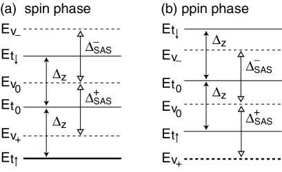
Figure 2: The energy levels are comprised of six levels. The spin phase or the ppin phase is realized for $E_{t_{\uparrow}}<E_{v_{+}}$ or $E_{v_{+}}<E_{t_{\uparrow}}$. Here, ${\Delta}_{\text{SAS}}^{\pm}={\frac{1}{2}}\left(\sqrt{4{\Delta}_{\text{SAS}}^{2}+\varepsilon_{\text{cap}}^{2}}\pm\varepsilon_{\text{cap}}\right)$

IV SU(4) Breaking and Topological Solitons

Isospin states in the $\nu=2$ BLQH system belong to the $\boldsymbol{6}$-dimensional irreducible representation of SU(4) as in (18). We restrict the Hamiltonian to this representation. In the SU(4)-invariant limit the Landau-site Hamiltonian is

$$H_{X}^{+}=-4\sum_{\langle i,j\rangle}J_{ij}^{+}\biggl{(}\widehat{\boldsymbol{T}}(i)\!\cdot\!\widehat{\boldsymbol{T}}(j)+{\frac{1}{8}}n(i)n(j)\biggr{)},$$ (31)

where $\widehat{\boldsymbol{T}}(j)$ are the fifteen generators of SU(4) in this representation. They are the spin-1 operators. We derive a field-theoretical Hamiltonian by taking a continuum limit. This can be done straightforwardlyEzawaX02B when Landau sites are taken on lattice points of a von Neumann latticevonNeumann55 ; Perelomov71 ; Bargmann71 ; Tao86 . It yields the SU(4) nonlinear sigma model,

$${\mathcal{H}}_{X}^{+}=2J^{+}\partial_{k}\widehat{\boldsymbol{T}}(\boldsymbol{x})\!\cdot\!\partial_{k}\widehat{\boldsymbol{T}}(\boldsymbol{x}),$$ (32)

where $J^{+}=\frac{1}{2}(J+J^{d})$ with

$$J=\frac{1}{16\sqrt{2\pi}}\frac{e^{2}}{4\pi\varepsilon\ell_{B}},$$ (33)

and

$$J^{d}=J\biggl{(}-\sqrt{\frac{2}{\pi}}\frac{d}{\ell_{B}}+\bigl{(}1+\frac{d^{2}}{\ell_{B}^{2}}\bigr{)}e^{d^{2}/2\ell_{B}^{2}}\bigl{\{}1-\text{erf}(d/\sqrt{2}\ell_{B})\bigr{\}}\biggr{)}.$$ (34)

All isospins are spontaneously polarized to lower this exchange energy. As far as the Hamiltonian (32) concerns, there are six degenerate states any one of which can be chosen as the ground state. It implies a spontaneous breaking of the SU(4) symmetry, giving rise to Goldstone modes and topological solitons.

The ground state is chosen actually by SU(4)-noninvariant interactions, as described in the previous section. Goldstone modes are made gapful and turned into pseudo-Goldstone modes. They are the soft waves in the system. When the explicit breaking is sufficiently small, the pattern of the spontaneous symmetry breaking provides us with an essential information on soft waves.

We study a spontaneous symmetry breaking in the spin phase. The ground state is a spin triplet and a ppin singlet. Let the spins be polarized to the $z$-direction. The residual symmetry is such one that keeps the ground state invariant. One residual symmetry is the rotation about the spin-$z$ axis, which is generated by the generator $S_{z}$. The ground state is also a ppin SU(2) singlet. Thus, the rotation in the ppin space generated by $P_{a}$ keeps the ground state invariant. In addition to them the combined one $2S_{z}P_{a}$ does not transform the ground state. These seven transformations generated by $S_{z},P_{a}$ and $2S_{z}P_{a}$ exhaust the residual symmetry, which is $U(1)\otimes SU(2)\otimes SU(2)$. They form the algebra,

$$[S_{z},J_{a}]=0,~{}~{}~{}~{}~{}~{}[S_{z},K_{b}]=0,~{}~{}~{}~{}~{}[J_{a},J_{b}]=i\epsilon_{abc}J_{c},$$

$$[K_{a},K_{b}]=i\epsilon_{abc}K_{c},~{}~{}~{}~{}~{}~{}[J_{a},K_{b}]=0,$$ (35)

where $J_{a}$ and $K_{a}$ are defined by

$$J_{a}=\frac{1}{2}(P_{a}+2S_{z}P_{a}),\qquad K_{a}=\frac{1}{2}(P_{a}-2S_{z}P_{a}).$$ (36)

The pattern of the symmetry breaking is

$$SU(4)\rightarrow U(1)\otimes SU(2)\otimes SU(2),$$ (37)

where the U(1) transformation is generated by $S_{z}$.

The target space is given by the coset space

$$G_{4,2}=SU(4)/[U(1)\otimes SU(2)\otimes SU(2)].$$ (38)

Here, $G_{N,k}$ is the complex Grassmannian manifold,

$$G_{N,k}=U(N)/[U(k)\otimes U(N-k)].$$ (39)

The dimension of the manifold $G_{4,2}$ is $15-7=8$ corresponding to the eight broken generators, $S_{x}$, $S_{y}$, $2S_{x}P_{a}$ and $2S_{y}P_{a}$. Thus, there emerge eight Goldstone modes associated with them.

There is a nontrivial mapping to this coset space,

$$\pi_{2}\left(G_{N,k}\right)=\pi_{1}(U(1))=\mathbb{Z},$$ (40)

where we have used $\pi_{2}(G/H)=\pi_{1}(H)$ (when G is simply connected) and $\pi_{n}(G\otimes G^{\prime})=\pi_{n}(G)\oplus\pi_{n}(G^{\prime})$. Consequently, there emerge topological solitons indexed by the topological number $\mathbb{Z}$. We call them $G_{4,2}$ skyrmions since they are associated with the Grassmannian manifold $G_{4,2}$: See also section V. Note that the $G_{4,1}$ skyrmion is the same object as the CP³ skyrmion discussed extensively in the previous paperEzawaX02B . The nontrivial mapping characterizing the soliton is the U(1) group generated by $S_{z}$.

Similarly we can study the spontaneous symmetry breaking in the ppin phase. The ground state is a ppin triplet and a spin singlet. For simplicity we consider the case, $d=0$, where all ppins are polarized to the $x$-direction by the tunneling interaction. The pattern of the symmetry breaking is the same as in the spin phase, as should be the case. The only difference is that the nontrivial mapping is the U(1) group generated by $P_{x}$. The seven residual symmetries are generated by $P_{x},S_{a}$ and $2S_{a}P_{x}$, while the eight broken symmetries are generated by $P_{y}$, $P_{z}$, $2S_{a}P_{y}$ and $2S_{a}P_{z}$.

V Grassmannian fields

There are fifteen generators in the nonlinear sigma model (32), but only eight of them are independent fields. To elucidate them we employ the composite boson (CB) theory of QH ferromagnetsEzawa99L ; Ezawa99JPSJ by attaching flux quanta to electronsGirvin87L ; Read89L ; Zhang89L . The CB field $\phi^{\sigma}(\boldsymbol{x})$ is defined by making a singular phase transformation to the electron field $\psi^{\sigma}(\boldsymbol{x})$,

$$\phi^{\sigma}(\boldsymbol{x})=e^{-ie\Theta(\boldsymbol{x})}\psi^{\sigma}(\boldsymbol{x}),$$ (41)

where the phase field $\Theta(\boldsymbol{x})$ is subject to the relation

$$\varepsilon_{ij}\partial_{i}\partial_{j}\Theta(\boldsymbol{x})=\Phi_{\text{D}}\rho(\boldsymbol{x}).$$ (42)

We introduce the normalized CB field $n^{\sigma}(\boldsymbol{x})$ by

$$\phi^{\sigma}(\boldsymbol{x})=\sqrt{\rho(\boldsymbol{x})}n^{\sigma}(\boldsymbol{x}),$$ (43)

obeying

$$\boldsymbol{n}^{\dagger}(\boldsymbol{x})\cdot\boldsymbol{n}(\boldsymbol{x})=\sum_{\sigma}n^{\sigma\dagger}(\boldsymbol{x})n^{\sigma}(\boldsymbol{x})=1.$$ (44)

Such a field is the CP³ fieldDAdda78NPB .

At $\nu=2$ there are two electrons per one Landau site. Let us introduce two CP³ fields $\boldsymbol{n}_{1}(\boldsymbol{x})$ and $\boldsymbol{n}_{2}(\boldsymbol{x})$ for them. They should be orthogonal one to another,

$$\boldsymbol{n}_{i}^{\dagger}(\boldsymbol{x})\cdot\boldsymbol{n}_{j}(\boldsymbol{x})=\delta_{ij},$$ (45)

because they describe hard-core bosons. Using a set of two CP³ fields subject to this normalization condition we consider a $4\times 2$ matrix field

$$Z(\boldsymbol{x})=(\boldsymbol{n}_{1},\boldsymbol{n}_{2}),$$ (46)

obeying

$$Z^{\dagger}Z=1.$$ (47)

Though we have introduced two fields $\boldsymbol{n}_{1}(\boldsymbol{x})$ and $\boldsymbol{n}_{2}(\boldsymbol{x})$, we cannot distinguish them quantum mechanically since they describe two electrons in the same Landau site. Namely, two fields $Z(\boldsymbol{x})$ and $Z^{\prime}(\boldsymbol{x})$ are indistinguishable physically when they are related by a local U(2) transformation $U(\boldsymbol{x})$,

$$Z^{\prime}(\boldsymbol{x})=Z(\boldsymbol{x})U(\boldsymbol{x}).$$ (48)

By identifying these two fields $Z(\boldsymbol{x})$ and $Z^{\prime}(\boldsymbol{x})$, the $4\times 2$ matrix field $Z(\boldsymbol{x})$ takes values on the Grassmannian manifold $G_{4,2}$ defined by (38). The field $Z(\boldsymbol{x})$ is no longer a set of two independent CP³ fields. It is a new object, called the Grassmannian field, carrying eight real degrees of freedom, as mentioned just below (39).

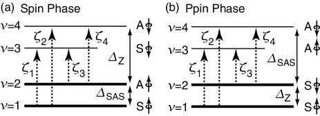
Figure 3: The lowest two energy levels are occupied in the ground state of the spin phase (a) and the ppin phase (b) at $\nu=2$. Small fluctuations are Goldstone modes $\zeta_{1}$, $\zeta_{2}$, $\zeta_{3}$ and $\zeta_{4}$.

The lowest-energy one-body electron state is the up-spin symmetric state. The second lowest energy state is either the up-spin antisymmetric state or the down-spin symmetric state [Fig.3]. It is convenient to use the CP³ field whose components are taken in the symmetric-antisymmetric basis,

$$n^{\text{S}\alpha}(\boldsymbol{x}) ={\frac{1}{\sqrt{2}}}\left(n^{\text{f}\alpha}(\boldsymbol{x})+n^{\text{b}\alpha}(\boldsymbol{x})\right),$$

$$n^{\text{A}\alpha}(\boldsymbol{x}) ={\frac{1}{\sqrt{2}}}\left(n^{\text{f}\alpha}(\boldsymbol{x})-n^{\text{b}\alpha}(\boldsymbol{x})\right),$$ (49)

where $\alpha=\uparrow,\downarrow$.

We first study the spin phase, where it is convenient to take the components of the CP³ field as [Fig.(a)]

$$\boldsymbol{n}=(n^{\text{S}\uparrow},n^{\text{A}\uparrow},n^{\text{S}\downarrow},n^{\text{A}\downarrow}).$$ (50)

In the ground state all up-spin states are occupied,

$$\boldsymbol{n}_{1}=(1,0,0,0),\quad\boldsymbol{n}_{2}=(0,1,0,0).$$ (51)

Accordingly the ground state is represented by the $G_{4,2}$ field as

$$Z_{\text{g}}=\left(\begin{array}[]{cc}1&0\\ 0&1\\ 0&0\\ 0&0\end{array}\right)U(\boldsymbol{x}).$$ (52)

We study perturbations around this ground state. Up to the second order of fluctuation fields, we may expand (46) as [Fig.3(a)]

$$Z=\left(\begin{array}[]{cc}1-\frac{1}{2}|\zeta_{1}|^{2}-\frac{1}{2}|\zeta_{2}|^{2}&-\frac{1}{2}\zeta_{1}^{\ast}\zeta_{3}-\frac{1}{2}\zeta_{2}^{\ast}\zeta_{4}\\ -\frac{1}{2}\zeta_{3}^{\ast}\zeta_{1}-\frac{1}{2}\zeta_{4}^{\ast}\zeta_{2}&1-\frac{1}{2}|\zeta_{3}|^{2}-\frac{1}{2}|\zeta_{4}|^{2}\\ \zeta_{1}&\zeta_{3}\\ \zeta_{2}&\zeta_{4}\end{array}\right)U(\boldsymbol{x}),$$ (53)

where $\zeta_{k}$ are the four complex Goldstone modes accompanied with the spontaneous SU(4) breaking (37). The Goldstone modes $\zeta_{1}$ and $\zeta_{4}$ are pure spin waves, while $\zeta_{2}$ and $\zeta_{3}$ are those mixing spins and pseudospins.

We can similarly analyze the ppin phase, where it is convenient to take the components of the CP³ field as [Fig.(b)]

$$\boldsymbol{n}=(n^{\text{S}\uparrow},n^{\text{S}\downarrow},n^{\text{A}\uparrow},n^{\text{A}\downarrow})$$ (54)

In the ground state all up-spin states are occupied,

$$\boldsymbol{n}_{1}=(1,0,0,0),\quad\boldsymbol{n}_{2}=(0,1,0,0).$$ (55)

The $G_{4,2}$ field is given by (52), and the eight Goldstone modes are parameterized as in (53) with this choice of the components of the CP³ field.

VI Soft Waves

We have argued that the dynamic fields are given by the Grassmannian field $Z(\boldsymbol{x})$ in the BLQH system at $\nu=2$. On the other hand, in the SU(4)-invariant limit the effective Hamiltonian is given by the nonlinear SU(4) sigma model (32) in terms of the SU(4) operator $\widehat{T}_{a}(\boldsymbol{x})$. By way of the relation

$$\widehat{T}_{a}={\frac{1}{2}}\text{Tr}[Z^{\dagger}\lambda_{a}Z]={\frac{1}{2}}\boldsymbol{n}_{1}^{\dagger}\lambda_{a}\boldsymbol{n}_{1}+{\frac{1}{2}}\boldsymbol{n}_{2}^{\dagger}\lambda_{a}\boldsymbol{n}_{2},$$ (56)

we are able to rewrite it into the well-known HamiltonianMacFarlane82PLB for the Grassmannian field,

$$\mathcal{H}_{X}^{+}=2J^{+}\text{Tr}\left[(\partial_{j}Z-iZK_{j})^{\dagger})(\partial_{j}Z-iZK_{j})\right],$$ (57)

where

$$K_{\mu}(\boldsymbol{x})=-iZ^{\dagger}(\boldsymbol{x})\partial_{\mu}Z(\boldsymbol{x}).$$ (58)

This Hamiltonian has the local U(2) gauge symmetry,

$$Z(\boldsymbol{x}) \rightarrow Z(\boldsymbol{x})U(\boldsymbol{x}),$$ (59a)

$$K_{\mu}(\boldsymbol{x}) \rightarrow U(\boldsymbol{x})^{\dagger}K_{\mu}(\boldsymbol{x})U(\boldsymbol{x})-iU(\boldsymbol{x})^{\dagger}\partial_{\mu}U(\boldsymbol{x}).$$ (59b)

The gauge field $$K_{\mu}$$ is not a dynamic field since it is an auxiliary field given by (58).

We study small fluctuations of the soft waves in the spin phase. Substituting the parametrization (53) of the Grassmannian field into the Hamiltonian (57), we expand it up to the second order,

$$\mathcal{H}_{X}^{+} = {2J^{+}}\sum_{i=1}^{4}\partial_{k}\zeta_{i}^{\dagger}(\boldsymbol{x})\partial_{k}\zeta_{i}(\boldsymbol{x})$$ (60)

$$= {\frac{J^{+}}{2}}\sum_{i=1}^{4}\bigl{\{}(\partial_{k}\sigma_{i})^{2}+(\partial_{k}\vartheta_{i})^{2}\bigr{\}},$$

where

$$\zeta_{i}(\boldsymbol{x})={\frac{1}{2}}\bigl{(}\sigma_{i}(\boldsymbol{x})+i\vartheta_{i}(\boldsymbol{x})\bigr{)}.$$ (61)

The equal-time commutation relation is

$$[\sigma_{i}(\boldsymbol{x}),\vartheta_{j}(\boldsymbol{y})]=2i\rho_{\Phi}^{-1}\delta_{ij}\delta(\boldsymbol{x}-\boldsymbol{y}),$$ (62)

where $\rho_{\Phi}=\frac{1}{2}\rho_{0}=1/(2\pi\ell_{B}^{2})$ represents the flux density. This Hamiltonian realizes the SU(4) symmetry nonlinearly. It describes four Goldstone modes associated with spontaneous symmetry breakdown of the SU(4) symmetry.

The SU(4) symmetry is broken explicitly but softly by various direct interactions. Relevant SU(2) operators are

$$\widehat{S}_{z} ={\frac{1}{2}}\text{Tr}\left[Z^{\dagger}\left(\begin{array}[]{cc}1_{2}&0\\ 0&-1_{2}\end{array}\right)Z\right]\simeq 1-\sum_{j=1}^{4}|\zeta_{j}|^{2},$$ (63c)

$$\widehat{P}_{x} ={\frac{1}{2}}\text{Tr}\left[Z^{\dagger}\left(\begin{array}[]{cc}1_{2}&0\\ 0&1_{2}\end{array}\right)Z\right]\simeq-|\zeta_{1}|^{2}+|\zeta_{3}|^{2},$$ (63f)

$$\widehat{P}_{z} ={\frac{1}{2}}\text{Tr}\left[Z^{\dagger}\left(\begin{array}[]{cc}\tau_{1}&0\\ 0&\tau_{1}\end{array}\right)Z\right]\simeq\text{Re}[(\zeta_{1}-\zeta_{4})(\zeta_{2}^{\ast}-\zeta_{3}^{\ast})],$$ (63i)

up to the second order of fluctuation fields, where the $$4\times 4$$ matrices are taken in the symmetric-asymmetric basis in accord with (53).

By taking into account of the SU(4)-noninvariant exchange interaction as well, the effective Hamiltonian is decomposed into four independent modes, $\mathcal{H}_{X}=\sum_{i=1}^{4}\mathcal{H}_{i}$, where

$$\mathcal{H}_{1}={\frac{J}{2}}\bigl{\{}(\partial_{k}\sigma_{1})^{2}+(\partial_{k}\vartheta_{1})^{2}\bigr{\}}+{\frac{{\Delta}_{\text{Z}}\rho_{\Phi}}{4}}\bigl{(}\sigma_{1}^{2}+\vartheta_{1}^{2}\bigr{)},$$ (64a)

$$\mathcal{H}_{4}={\frac{J}{2}}\bigl{\{}(\partial_{k}\sigma_{4})^{2}+(\partial_{k}\vartheta_{4})^{2}\bigr{\}}+{\frac{{\Delta}_{\text{Z}}\rho_{\Phi}}{4}}\bigl{(}\sigma_{4}^{2}+\vartheta_{4}^{2}\bigr{)},$$ (64b)

$$\mathcal{H}_{2}={\frac{J^{d}}{2}}\bigl{\{}(\partial_{k}\sigma_{2})^{2}+(\partial_{k}\vartheta_{2})^{2}\bigr{\}}+{\frac{({\Delta}_{\text{Z}}+{\Delta}_{\text{SAS}})\rho_{\Phi}}{4}}\bigl{(}\sigma_{2}^{2}+\vartheta_{2}^{2}\bigr{)},$$ (64c)

$$\mathcal{H}_{3}={\frac{J^{d}}{2}}\bigl{\{}(\partial_{k}\sigma_{3})^{2}+(\partial_{k}\vartheta_{3})^{2}\bigr{\}}+{\frac{|{\Delta}_{\text{Z}}-{\Delta}_{\text{SAS}}|\rho_{\Phi}}{4}}\bigl{(}\sigma_{3}^{2}+\vartheta_{3}^{2}\bigr{)}.$$ (64d)

They describe four independent soft waves, which are pseudo-Goldstone modes by acquiring gaps. They have finite coherence lengths (correlation lengths),

$$\xi_{1} =\xi_{4}=\ell_{B}\sqrt{{\frac{4\pi J}{{\Delta}_{\text{Z}}}}},$$ (65a)

$$\xi_{\text{2}} =\ell_{B}\sqrt{{\frac{4\pi J^{d}}{{\Delta}_{\text{Z}}+{\Delta}_{\text{SAS}}}}},$$ (65b)

$$\xi_{\text{3}} =\ell_{B}\sqrt{{\frac{4\pi J^{d}}{|{\Delta}_{\text{Z}}-{\Delta}_{\text{SAS}}|}}}.$$ (65c)

The two modes $$\zeta_{1} \zeta_{4} \zeta_{\text{3}} {\Delta}_{\text{Z}}={\Delta}_{\text{SAS}} d\rightarrow\infty \xi_{2}\rightarrow 0 \xi_{3}\rightarrow 0 J^{d}\rightarrow 0 \zeta_{2} \zeta_{3}$$ and are degenerate. The mode becomes gapless at , which signals the breakdown of the spin phase due to an infrared catastrophe. As we find and since , which implies the disappearance of the Goldstone modes and due to the decoupling of the bilayer system into the two monolayer systems.

We may perform a similar analysis in the ppin phase. Relevant operators for the direct interactions are

$$\hat{S}_{z} \simeq-|\zeta_{2}|^{2}+|\zeta_{3}|^{2},$$ (66a)

$$\hat{P}_{x} \simeq 1-(|\zeta_{1}|^{2}+|\zeta_{2}|^{2}+|\zeta_{3}|^{2}+|\zeta_{4}|^{2}),$$ (66b)

$$\hat{P}_{z} \simeq\frac{1}{2}(\zeta_{1}^{\dagger}+\zeta_{1}+\zeta_{4}^{\dagger}+\zeta_{4}).$$ (66c)

The effective Hamiltonian is decomposed into four independent modes, $$\mathcal{H}_{\text{X}}=\sum_{i=1}^{4}\mathcal{H}_{i} \mathcal{H}_{2} \mathcal{H}_{3} \zeta_{\text{3}} {\Delta}_{\text{Z}}={\Delta}_{\text{SAS}} \mathcal{H}_{1}$$. The Hamiltonians and are given by the same Hamiltonians (64c) and (64d), respectively. The coherence lengths are given by (65b) and (65c). The mode becomes gapless at , which signals the breakdown of the ppin phase due to an infrared catastrophe. On the other hand, the Hamiltonian reads

$$\mathcal{H}_{1}= {\frac{J}{2}}(\partial_{k}\sigma_{1})^{2}+{\frac{J^{d}}{2}}(\partial_{k}\vartheta_{1})^{2}+{\frac{\varepsilon_{\text{cap}}\rho_{\Phi}}{4}}\sigma_{1}^{2}$$

$$+{\frac{{\Delta}_{\text{SAS}}\rho_{\Phi}}{4}}\bigl{(}\sigma_{1}^{2}+\vartheta_{1}^{2}\bigr{)}\boldsymbol{\ }.$$ (67)

The Hamiltonians $\mathcal{H}_{4}$ is given by the same Hamiltonian as $\mathcal{H}_{1}$ with the replacement of the fields $(\sigma_{1},\vartheta_{1})$ by $(\sigma_{4},\vartheta_{4})$. There are two coherent lengths associated with the $\sigma$ field and the $\vartheta$ field,

$$\xi_{1}^{\vartheta} =\xi_{4}^{\vartheta}=\ell_{B}\sqrt{{\frac{4\pi J^{d}}{{\Delta}_{\text{SAS}}}}},$$ (68a)

$$\xi_{1}^{\sigma} =\xi_{4}^{\sigma}=\ell_{B}\sqrt{{\frac{4\pi J}{\varepsilon_{\text{cap}}+{\Delta}_{\text{SAS}}}}}.$$ (68b)

The ground state of these modes (67) is a squeezed state as in the $$\nu=1 \xi_{1} \xi_{4} \nu=1$$ caseEzawaX02B , where the coherence lengths are different between the conjugate variables. A new feature is that the interlayer tunneling modes and mediate the Josephson-like effect as in the caseEzawa92IJMPB ; BookEzawa .

VII Grassmannian $G_{4,2}$ Skyrmions

The homotopy theorem (40) guarantees the existence of topological solitons ($G_{4,2}$ skyrmions). The topological charge is definedMacFarlane82PLB as a gauge invariant by

$$Q={\frac{i}{2\pi}}\int d^{2}x\epsilon_{jk}\text{Tr}\left[(\partial_{j}Z-iZK_{j})^{\dagger}(\partial_{k}Z-iZK_{k})\right].$$ (69)

It is a topological invariant since it is equal to

$$Q={\frac{i}{2\pi}}\int d^{2}x\epsilon_{jk}\text{Tr}\left[(\partial_{j}Z)^{\dagger}(\partial_{k}Z)\right].$$ (70)

We rewrite it with the use of (46) as

$$Q={\frac{i}{2\pi}}\int d^{2}x\epsilon_{jk}\left[(\partial_{j}\boldsymbol{n}_{1})^{\dagger}\cdot(\partial_{k}\boldsymbol{n}_{1})+(\partial_{j}\boldsymbol{n}_{2})^{\dagger}\cdot(\partial_{k}\boldsymbol{n}_{2})\right].$$ (71)

It is the sum of the topological charges associated with the CP³ fields $\boldsymbol{n}_{1}$ and $\boldsymbol{n}_{2}.$Hence, the $G_{4,2}$ skyrmion consists of CP³ skyrmions,

$$n_{k}^{\sigma}(\boldsymbol{x})=\frac{1}{\sqrt{\sum|\omega_{k}^{\sigma}(z)|}}\omega_{k}^{\sigma}(z),$$ (72)

excited in the front and back layers in the spin phase, or in the up-spin and down-spin states in the ppin phase. Here, $\omega_{k}^{\sigma}(z)$ are arbitrary analytic functions.

For definiteness we consider the spin phase, where we now choose $\boldsymbol{n}_{k}=(n_{k}^{\text{f}\uparrow},n_{k}^{\text{b}\uparrow},n_{k}^{\text{f}\downarrow},n_{k}^{\text{b}\downarrow})$. The simplest soliton would be a set of one CP³ skyrmion in the front layer and the ground state in the back layer, $\boldsymbol{n}_{1}=(z,\kappa,0,0)/\sqrt{|z|^{2}+\kappa^{2}}$ and $\boldsymbol{n}_{2}=(0,1,0,0)$, or

$$Z_{\text{sky}}^{1}=\frac{1}{\sqrt{|z|^{2}+\kappa^{2}}}\left(\begin{array}[]{cc}z&0\\ 0&\sqrt{|z|^{2}+\kappa^{2}}\\ \kappa&0\\ 0&0\end{array}\right)U(\boldsymbol{x}),$$ (73)

for which the topological charge (69) is $Q=1$. The next simplest would be a set of two CP³ skyrmions both in the front and back layers,

$$Z_{\text{sky}}^{2}=\frac{1}{\sqrt{|z|^{2}+\kappa^{2}}}\left(\begin{array}[]{cc}z&0\\ 0&z\\ \kappa&0\\ 0&k\end{array}\right)U(\boldsymbol{x}),$$ (74)

for which $Q=2$. We now argue that the simplest G_4,2 skyrmion (73) is ruled out since it is not confined within the lowest Landau level.

The Landau-site Hamiltonian (31) has been derived by requiring the LLL condition. However, the nonlinear sigma model (32), obtained after taking a continuum limit, is an ordinary local Hamiltonian, and the CP^N-1 field (43) is an ordinary field without the LLL projection. Hence, it is necessary to require the LLL condition on the soliton statesBookEzawa .

The condition requires the kinetic Hamiltonian to be quenched on the state, which readsEzawa99L

$$\frac{\partial}{\partial z^{\ast}}\varphi^{\sigma}(\boldsymbol{x})|\Phi\rangle=0.$$ (75)

Here $\varphi^{\sigma}(\boldsymbol{x})$ is the dressed CB fieldEzawa99L ; Read89L defined by

$$\varphi^{\sigma}(\boldsymbol{x})=e^{-\mathcal{A}(\boldsymbol{x})}\phi^{\sigma}(\boldsymbol{x}),$$ (76)

where $\phi^{\sigma}(\boldsymbol{x})$ is the CB field (41), while ${\mathcal{A}}(\boldsymbol{x})$ is an auxiliary field determined by

$$\boldsymbol{\nabla}^{2}{\mathcal{A}}(\boldsymbol{x})=2\pi\left(\rho(\boldsymbol{x})-\rho_{0}\right),$$ (77)

as follows from the condition (42) on the phase field. We take a coherent state of $\varphi^{\sigma}(\boldsymbol{x})$, for which (75) implies

$$\varphi^{\sigma}(\boldsymbol{x})|\Phi\rangle=\omega^{\sigma}(z)|\Phi\rangle,$$

where $\omega^{\sigma}(z)$ is an analytic function. The coherent state $|\Phi\rangle$ must be an eigenstate of the density operator $\rho(\boldsymbol{x})$ and a coherent state of the CP³ field $\boldsymbol{n}(\boldsymbol{x})$ since they commute with each other. Hence we have

$$e^{-\mathcal{A}^{\text{cl}}(\boldsymbol{x})}\sqrt{\rho^{\text{cl}}(\boldsymbol{x})}n^{\text{cl(}\sigma)}(\boldsymbol{x})=\omega^{\sigma}(z),$$ (78)

where $\mathcal{A}^{\text{cl}}(\boldsymbol{x})$, $\rho^{\text{cl}}(\boldsymbol{x})$ and $n^{\text{cl(}\sigma)}(\boldsymbol{x})$ are classical fields. This is the LLL condition for soliton states.

At $\nu=2$ we have

$$\boldsymbol{n}(\boldsymbol{x})|\Phi\rangle=\boldsymbol{n}^{\text{cl}}(\boldsymbol{x})|\Phi\rangle=\left[\boldsymbol{n}_{1}^{\text{cl}}(\boldsymbol{x})+\boldsymbol{n}_{2}^{\text{cl}}(\boldsymbol{x})\right]|\Phi\rangle,$$ (79)

together with $\boldsymbol{n}_{i}^{\text{cl}}(\boldsymbol{x})\cdot\boldsymbol{n}_{j}^{\text{cl}}(\boldsymbol{x})=\delta_{ij}$ and

$$\rho(\boldsymbol{x})|\Phi\rangle=\rho^{\text{cl}}(\boldsymbol{x})|\Phi\rangle=[\rho_{1}^{\text{cl}}(\boldsymbol{x})+\rho_{2}^{\text{cl}}(\boldsymbol{x})]|\Phi\rangle.$$ (80)

Keeping in mind the local U(2) invariance we work in such a gauge that $U(\boldsymbol{x})=1$ in (73) and (74). We may solve (78) as

$$n^{\text{cl(}\sigma)}(\boldsymbol{x})=\frac{\sqrt{2}}{\sqrt{\sum|\omega^{\sigma}(x)|^{2}}}\omega^{\sigma}(z).$$ (81)

Comparing this with (72) we conclude $\sum_{\sigma}|\omega_{1}^{\sigma}(z)|^{2}=\sum_{\sigma}|\omega_{2}^{\sigma}(z)|^{2}$ and $\omega^{\sigma}(z)=\omega_{1}^{\sigma}(z)+\omega_{2}^{\sigma}(z)$. Therefore, for each component the LLL condition (78) holds and we obtain from (77) that

$${\frac{1}{4\pi}}\boldsymbol{\nabla}^{2}\ln\rho^{\text{cl}}(\boldsymbol{x})-\rho^{\text{cl}}(\boldsymbol{x})+\rho_{0}=j_{\text{sky}}^{0}(\boldsymbol{x})$$ (82)

with

$$j_{\text{sky}}^{0}(\boldsymbol{x}) = {\frac{1}{4\pi}}\boldsymbol{\nabla}^{2}\ln\sum_{\sigma}|\omega_{1}^{\sigma}(z)|^{2}$$ (83)

$$= {\frac{1}{4\pi}}\boldsymbol{\nabla}^{2}\ln\sum_{\sigma}|\omega_{2}^{\sigma}(z)|^{2}.$$

It is easy to see that the topological charge (71) is given by $Q=2\int d^{2}x\,j_{\text{sky}}^{0}(\boldsymbol{x})$.

The G_4,2 skyrmion has a general expression,

$$Z_{\text{sky}}=\frac{1}{\sqrt{\sum_{\sigma}|\omega_{1}^{\sigma}(z)|^{2}}}\left(\begin{array}[]{cc}\omega_{1}^{\text{f}\uparrow}(z)&\omega_{2}^{\text{f}\uparrow}(z)\\ \omega_{1}^{\text{f}\downarrow}(z)&\omega_{2}^{\text{f}\downarrow}(z)\\ \omega_{1}^{\text{b}\uparrow}(z)&\omega_{2}^{\text{b}\uparrow}(z)\\ \omega_{1}^{\text{b}\downarrow}(z)&\omega_{2}^{\text{b}\downarrow}(z)\end{array}\right).$$ (84)

This rules out the soliton (73) with $Q=1$. The simplest G_4,2 skyrmion is given by (74), which describes a pair of CP³ skyrmions excited in both layers. We call it a biskyrmion.

We emphasize this peculiar situation by recalling the formula (43) to introduce the normalized CB field $\boldsymbol{n(x)}$. It is essential that the total electron density $\rho(\boldsymbol{x})$ is common to all the four components: Otherwise the SU(4) symmetry is explicitly broken by hand. Even if we try to excite a skyrmion only in the front layer, the density modulation associated with it affects equally electrons in the back layer as far as the LLL condition (78) is respected. In a genuine BLQH system it is impossible to have a skyrmion excitation in the front layer and the ground state in the back layer simultaneously: See section IX for more details on this point.

Finally we note that the G_4,2 skyrmion is a BPS soliton of the exchange Hamiltonian (57). Indeed, the following inequalityMacFarlane82PLB holds between the exchange energy (57) and the topological charge (69),

$$E_{X}\geqq 4\pi J^{+}Q,$$ (85)

where the equality is achieved by the G_4,2 skyrmion (84).

A completely analogous analysis is made in the ppin phase by choosing $\boldsymbol{n}=(n^{\text{S}\uparrow},n^{\text{S}\downarrow},n^{\text{A}\uparrow},n^{\text{A}\downarrow})$. We achieve the same conclusion that the lightest topological excitation is a biskyrmion.

VIII Spin-1 Sigma Models for Biskyrmions

We have argued that charged excitations are biskyrmions in the $\nu=2$ BLQH system. We have described them in terms of the Grassmannian field $Z(\boldsymbol{x}).$ We now represent them in terms of the SU(4) sigma field by way of the relation (56).

We first treat the spin phase. We calculate the SU(4) generators $\widehat{T}_{a}(\boldsymbol{x})$ by using the biskyrmion configuration (74) in (56), from which the fifteen operators $\widehat{S}_{a}$, $\widehat{P}_{a}$ and $2\widehat{S}_{a}\widehat{P}_{b}$ are derived with the aid of the relations (15). We find that $\widehat{P}_{a}=2\widehat{S}_{a}\widehat{P}_{b}=0$ and that $\widehat{S}_{a}$ are given by the well-known formula of the O(3) skyrmion,

$$\widehat{S}_{x} =\frac{2\kappa|z|}{|z|^{2}+\kappa^{2}}\cos\theta,\quad\widehat{S}_{y}=-\frac{2\kappa|z|}{|z|^{2}+\kappa^{2}}\sin\theta,$$

$$\widehat{S}_{z} =\frac{|z|^{2}-\kappa^{2}}{|z|^{2}+\kappa^{2}}.$$ (86)

It is easy to see that this biskyrmion configuration is purely spin-like and expanded by three states (20). We call it the spin biskyrmion.

We define bosonic operators $t_{a}$ on the lattice by

$$t_{a}^{\dagger}(i)|0\rangle=|t_{a}\rangle_{i}.$$ (87)

They satisfy hard-core bosonic commutation relations and describe Schwinger bosonsSachdev90B . In the field-theoretical limit we have

$$t_{\uparrow}(\boldsymbol{x}) =n^{\text{f}\uparrow}(\boldsymbol{x})n^{\text{b}\uparrow}(\boldsymbol{x}),$$

$$t_{0}(\boldsymbol{x}) =\frac{1}{\sqrt{2}}\bigl{(}n^{\text{f}\uparrow}(\boldsymbol{x})n^{\text{b}\downarrow}(\boldsymbol{x})+n^{\text{f}\downarrow}(\boldsymbol{x})n^{\text{b}\uparrow}(\boldsymbol{x})\bigr{)},$$

$$t_{\downarrow}(\boldsymbol{x}) =n^{\text{f}\downarrow}(\boldsymbol{x})n^{\text{b}\downarrow}(\boldsymbol{x}),$$ (88)

which read

$$\boldsymbol{t}(\boldsymbol{x})=(t_{\uparrow},t_{0},t_{\downarrow})=\frac{1}{|z|^{2}+\kappa^{2}}(z^{2},\sqrt{2}z\kappa,\kappa^{2})$$ (89)

on the biskyrmion configuration (74). The spin-1 field is given by

$$\widehat{S}_{a}(\boldsymbol{x})=\boldsymbol{t}^{\dagger}(\boldsymbol{x})\widehat{\tau}_{a}\boldsymbol{t}(\boldsymbol{x}),$$ (90)

where $\widehat{\tau}_{a}$ are the SU(2) generators in the adjoint representation,

$$\widehat{\boldsymbol{\tau}}\equiv\biggl{\{}\frac{1}{\sqrt{2}}\begin{pmatrix}0&1&0\\ 1&0&1\\ 0&1&0\end{pmatrix},\frac{1}{\sqrt{2}}\begin{pmatrix}0&{-i}&0\\ {i}&0&{-i}\\ 0&{i}&0\end{pmatrix},\begin{pmatrix}1&0&0\\ 0&0&0\\ 0&0&-1\end{pmatrix}\biggr{\}}.$$ (91)

Calculating (90) with (88) and (89), we reproduce the skyrmion configuration (86). Hence, the Grassmannian G_4,2 skyrmion (74) in the spin phase is equal to the O(3) skyrmion in the spin sector.

We reduce the Hamiltonian (16) to the spin sector. Because $\langle\widehat{P}_{a}\rangle=\langle\widehat{S}_{a}\widehat{P}_{b}\rangle=0$, we obtain that

$$H_{X}=-2\sum_{\langle i,j\rangle}J_{ij}\widehat{\boldsymbol{S}}(i)\!\cdot\!\widehat{\boldsymbol{S}}(j).$$ (92)

Taking the continuum limit and including the direct interactions, we find

$${\mathcal{H}}_{\text{spin}}=J\partial_{k}\widehat{\boldsymbol{S}}(\boldsymbol{x})\!\cdot\!\partial_{k}\widehat{\boldsymbol{S}}(\boldsymbol{x})+{\mathcal{H}}_{\text{Coulomb}}+{\Delta}_{\text{Z}}\bar{\rho}_{B}\left(1-\widehat{S}_{z}(\boldsymbol{x})\right),$$ (93)

where ${\mathcal{H}}_{\text{Coulomb}}$ stands for the direct Coulomb energy. The O(3) skyrmion (86) is the BPS soliton of the O(3)-nonlinear-sigma-model part of this Hamiltonian. The total Hamiltonian (93) is very similar to the one in the monolayer QH system at $\nu=1$ with the replacement of the spin-${\frac{1}{2}}$ field by the spin-$1$ field.

The excitation energy of the biskyrmion is easily calculable based on (93) as in the $\nu=1$ monolayer QH system Ezawa99JPSJ . The skyrmion scale $\kappa$ is determined to optimize the Coulomb energy and the Zeeman energy. It is to be remarked that the spin biskyrmion is insensible to the interlayer stiffness $J^{d}$.

We may similarly discuss the ppin phase, where only $\widehat{P}_{a}$ is nonvanishing for the biskyrmion configuration. The biskyrmion turns out to be the O(3) skyrmion,

$$\widehat{P}_{y} =\frac{2\kappa|z|}{|z|^{2}+\kappa^{2}}\cos\theta,\quad\widehat{P}_{z}=-\frac{2\kappa|z|}{|z|^{2}+\kappa^{2}}\sin\theta,$$

$$\widehat{P}_{x} =\frac{|z|^{2}-\kappa^{2}}{|z|^{2}+\kappa^{2}}.$$ (94)

We call it the ppin biskyrmion. The effective Hamiltonian restricted to the ppin sector is

$${\mathcal{H}}_{\text{ppin}} =J^{d}\bigl{\{}\partial_{k}\widehat{\boldsymbol{P}}(\boldsymbol{x})\!\cdot\!\partial_{k}\widehat{\boldsymbol{P}}(\boldsymbol{x})\bigr{\}}_{xy}+J\partial_{k}\widehat{P}_{z}(\boldsymbol{x})\cdot\partial_{k}\widehat{P}_{z}(\boldsymbol{x})$$

$$+{\mathcal{H}}_{\text{Coulomb}}+{\Delta}_{\text{SAS}}\bar{\rho}_{B}\left(1-\widehat{P}_{x}(\boldsymbol{x})\right),$$ (95)

where ${\mathcal{H}}_{\text{Coulomb}}$ stands for the direct Coulomb energy including the capacitance effect. The total Hamiltonian is quite similar to that in the spin-frozen BLQH system at $\nu=1$ with the replacement of the ppin-${\frac{1}{2}}$ field with the ppin-$1$ field.

IX Two Monolayer Systems

It is intriguing that a quasiparticle is a biskyrmion at $\nu=2$. However, it is clear intuitively that a quasiparticle is a simple skyrmion excited in one of the two layers even at $\nu=2$ if the two layers are sufficiently separated. We have studied previouslyEzawaX02B ; RJ the criterion for a system at $\nu=1$ to be a genuine bilayer system or a set of two monolayer systems. It is determined by the local symmetry present in the Hamiltonian. Let us recapitulate the argumentEzawaX02B and extend it to the system at $\nu=2$.

We first examine the local symmetry of the direct interaction (24). It is given by a direct product of two U(1) symmetries, U^↑(1)$\otimes$U^↓(1),

$$\begin{pmatrix}\psi^{\text{f}\uparrow}(\boldsymbol{x})\\ \psi^{\text{b}\uparrow}(\boldsymbol{x})\end{pmatrix} \longrightarrow e^{i\alpha(\boldsymbol{x})}\begin{pmatrix}\psi^{\text{f}\uparrow}(\boldsymbol{x})\\ \psi^{\text{b}\uparrow}(\boldsymbol{x})\end{pmatrix},$$

$$\begin{pmatrix}\psi^{\text{f}\downarrow}(\boldsymbol{x})\\ \psi^{\text{b}\downarrow}(\boldsymbol{x})\end{pmatrix} \longrightarrow e^{i\beta(\boldsymbol{x})}\begin{pmatrix}\psi^{\text{f}\downarrow}(\boldsymbol{x})\\ \psi^{\text{b}\downarrow}(\boldsymbol{x})\end{pmatrix}.$$ (96)

The exchange interaction (16) breaks this into a single U(1) symmetry,

$$\psi^{\sigma}(\boldsymbol{x})\longrightarrow e^{i\alpha(\boldsymbol{x})}\psi^{\sigma}(\boldsymbol{x}).$$ (97)

Note that this is the case even if $J^{d}=0$ provided $J\neq 0$. It is the exact local symmetry of the total Hamiltonian. Corresponding to this U(1) symmetry, we have introduced the normalized CB field $n^{\sigma}(\boldsymbol{x})$ in (43), or

$$\phi^{\sigma}(\boldsymbol{x})=\sqrt{\rho(\boldsymbol{x})}n^{\sigma}(\boldsymbol{x}).$$ (98)

It is the CP³ field containing 3 independent complex fields, because one real field is eliminated by the constraint (44) and furthermore the U(1) phase field is not dynamic due to the local U(1) symmetry (97). At $\nu=2$ we introduce a set of two CP³ fields for two electrons in one Landau site with the U(2) local symmetry (59b). The set turns out to be a Grassmannian G_4,2 field with four independent complex fields. Topological solitons are biskyrmions.

We next consider a system where the two layers are separated sufficiently so that there are no interlayer exchange interaction ($J^{d}=0$) nor the tunneling interaction (${\Delta}_{\text{SAS}}=0$). Then, the total Hamiltonian is invariant under two local transformations, U${}^{\text{f}}$(1) and U${}^{\text{b}}$(1), which act on electrons on the two layers independently,

$$\begin{pmatrix}\psi^{\text{f}\uparrow}(\boldsymbol{x})\\ \psi^{\text{f}\downarrow}(\boldsymbol{x})\end{pmatrix} \longrightarrow e^{i\alpha(\boldsymbol{x})}\begin{pmatrix}\psi^{\text{f}\uparrow}(\boldsymbol{x})\\ \psi^{\text{f}\downarrow}(\boldsymbol{x})\end{pmatrix},$$

$$\begin{pmatrix}\psi^{\text{b}\uparrow}(\boldsymbol{x})\\ \psi^{\text{b}\downarrow}(\boldsymbol{x})\end{pmatrix} \longrightarrow e^{i\beta(\boldsymbol{x})}\begin{pmatrix}\psi^{\text{b}\uparrow}(\boldsymbol{x})\\ \psi^{\text{b}\downarrow}(\boldsymbol{x})\end{pmatrix}.$$ (99)

Corresponding to these two U(1) symmetries, we should introduced two normalized CB fields by

$$\phi^{\text{f}\alpha}(\boldsymbol{x})=\sqrt{\rho^{\text{f}}(\boldsymbol{x})}n^{\text{f}\alpha}(\boldsymbol{x}),\quad\phi^{\text{b}\alpha}(\boldsymbol{x})=\sqrt{\rho^{\text{b}}(\boldsymbol{x})}n^{\text{b}\alpha}(\boldsymbol{x}),$$ (100)

where $\alpha=\uparrow,\downarrow$ and

$$\sum_{\alpha=\uparrow\downarrow}n^{\text{f}\alpha\dagger}(\boldsymbol{x})n^{\text{f}\alpha}(\boldsymbol{x})=\sum_{\alpha=\uparrow\downarrow}n^{\text{b}\alpha\dagger}(\boldsymbol{x})n^{\text{b}\alpha}(\boldsymbol{x})=1.$$ (101)

We have a set of two CP¹ fields as the basic fields, each of which is the dynamic field for each layer at $\nu=2$. Topological solitons are simple skyrmions.

It is interesting to consider a case without the interlayer exchange interaction ($J^{d}\simeq 0$) but with a nonnegligible tunneling interaction (${\Delta}_{\text{SAS}}\not=0$). The basic field is the CP³ field because the Hamiltonian possesses only the local U(1) symmetry (97). Hence, we have the G_4,2 field at $\nu=2$. It is a genuine BLQH system and topological solitons are biskyrmions.

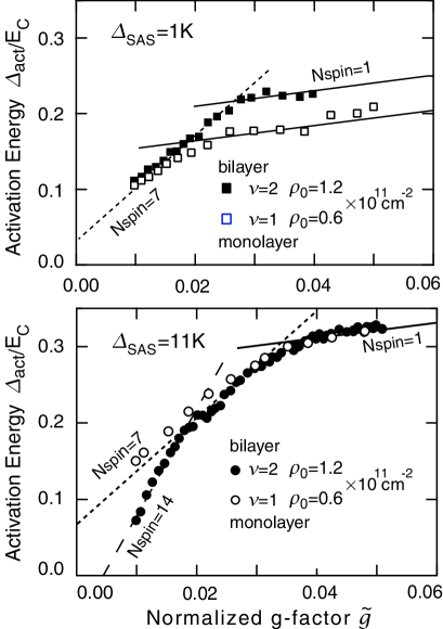
Figure 4: The activation energy is given in the $\nu=2$ BLQH state (solid marks) and the $\nu=1$ monolayer QH state (open marks). The data are taken from Kumada et al.Kumada00L . The vertical axis is the activation energy $\Delta_{\text{act}}$ in units of $E_{\text{C}}^{0}\equiv e^{2}/4\pi\varepsilon\ell_{B}$. The horizontal axis is the normalized $g$-factor $\widetilde{g}\equiv{\Delta}_{\text{Z}}/E_{\text{C}}^{0}$. The number of flipped spins is given by the slope of the data $\text{N}_{\text{spin}}=\partial\Delta_{\text{act}}/\partial\widetilde{g}$.

We wish to do a thinking experiment to make it convincing that a biskyrmion is excited even for $J^{d}\simeq 0$ provided ${\Delta}_{\text{SAS}}\neq 0$. We start with the SU(4)-invariant limit of the exchange interaction ($J^{d}\simeq J$), where a biskymion must be excited. We question what would happen as $J^{d}$ is decreased. As far as ${\Delta}_{\text{SAS}}$ is significant, two electrons in one Landau site are indistinguishable, and hence we need the Grassmannian field $Z(\boldsymbol{x})$ to describe the system. Furthermore, the spin biskyrmion (86) is insensible to the interlayer stiffness $J^{d}$, as we have remarked, because it is governed by the Hamiltonian (93). Hence, nothing would happen for the spin biskyrmion as $J^{d}\rightarrow 0$. It is to be stressed that the existence of topological solitons is the property of the Grassmannian manifold and not the property of the Hamiltonian (57). When $J^{d}\simeq 0$ the Grassmannian soliton is not the BPS state of the Hamiltonian, but its very existence is guaranteed by the homotopy theorem (40).

Topological solitons arise as quasiparticles (charged excitations). Their excitation energy is observed as the activation energy. By measuring it as a function of the tilting angle $\Theta$, we can tell how many spins are flipped by one topological solitonSchmeller95L . Kumada et al.Kumada00L made a careful measurement of activation energy by using two bilayer samples with a large tunneling gap (${\Delta}_{\text{SAS}}\simeq 11$ K) and a small tunneling gap (${\Delta}_{\text{SAS}}\simeq 1$ K). These two samples have precisely the same sample parameters except for the tunneling gap, where $J^{d}/J=0.15$ with use of (34). Thus, $J^{d}$ is quite small compared with $J$. They have also measured activation energy in the monolayer limit of the same samples. (The monolayer state is constructed by emptying the back layer by tuning the bias voltage in the bilayer sample. The total electron density in the bilayer system is controlled so that it is precisely twice of that in the monolayer system.) They have found 7 flipped spins in the 1K-sample while 14 flipped spins in the 11K-sample when the tilting angle is small [Fig.4]. When the tilting angle becomes large, the number of flipped spins makes a transition from 14 to 7 in the 11K-sample. This is understood as follows. As the sample is tilted, the tunneling gap is knownHu92B to decrease as

$${\Delta}_{\text{SAS}}(\Theta)={\Delta}_{\text{SAS}}\exp\{-(d/2\ell_{B})^{2}\tan^{2}\Theta\}.$$ (102)

In Fig.4 the transition occurs at $\Theta=60^{\circ}$, where ${\Delta}_{\text{SAS}}\simeq 2$K. It is small enough compared with other interactions and would be practically negligible. They have also confirmed 7 flipped spins in the monolayer limit of both samples. (Only one spin is flipped in all cases for a sufficiently large tilting angle, where a vortex is excited in one of the layers since the tunneling gap becomes so small and the Zeeman effect becomes so large.) These facts are consistent with our conclusion that biskyrmions (simple skyrmion) are excited in a sample with a large (negligible) tunneling gap.

X Summary

We have investigated the BLQH systems at $\nu=2$. There are three phases, i.e. the spin phase, the ppin phase and the canted phase. Experimentally the spin and ppin phases are clearly observed. We have presented a field-theoretical formulation of these two phases, and analyzed soft waves and topological excitations. We have shown that the dynamic field is the Grassmannian G_4,2 field, which is a set of two CP³ fields but contains only four complex independent fields. Accordingly there are four independent soft waves (pseudo-Goldstone modes) as neutral low energy excitations. We have also shown that there are topological excitations as charged excitations: They are biskyrmions comprised of two simple skyrmions in the two layers and possess the electric charge $2e$. This conclusion on charged excitations is confirmed by a recent experimental resultKumada00L in the spin phase at $\nu=2$, where the number of flipped spins is found to be twice as large as that at $\nu=1$ for a sample with large ${\Delta}_{\text{SAS}}$.

References

• (1) S. Das Sarma and A. Pinczuk (eds), Perspectives in Quantum Hall Effects (Wiley, 1997).
• (2) Z.F. Ezawa, Quantum Hall Effects: Field Theoretical Approach and Related Topics (World Scientifics, 2000).
• (3) S.L. Sondhi, A. Karlhede, S.A. Kivelson and E.H. Rezayi, Phys. Rev. B 47 (1993) 16419.
• (4) S.E. Barrett, G. Dabbagh, L.N. Pfeiffer, K.W. West and R. Tycko, Phys. Rev. Lett. 74 (1995) 5112.
• (5) E.H. Aifer, B.B. Goldberg and D.A. Broido, Phys. Rev. Lett. 76 (1996) 680.
• (6) A. Schmeller, J.P. Eisenstein, L.N. Pfeiffer and K.W. West, Phys. Rev. Lett. 75 (1995) 4290.
• (7) Z.F. Ezawa, Phys. Rev. B 55 (1997) 7771.
• (8) Z.F. Ezawa, Phys. Rev. Lett. 82 (1999) 3512.
• (9) I.B. Spielman, J.P. Eisenstein, L.N. Pfeiffer and K.W. West, Phys. Rev. Lett. 84 (2000) 5808.
• (10) Z.F. Ezawa and A. Iwazaki, Int. J. Mod. Phys. B 6 (1992) 3205; Phys. Rev. B 47 (1993) 7295; 48 (1993) 15189.
• (11) K. Moon, H. Mori, K. Yang, S.M. Girvin, A.H. MacDonald, L. Zheng, D. Yoshioka and S-C. Zhang, Phys. Rev. B 51 (1995) 5138.
• (12) Z.F. Ezawa and K. Hasebe, Phys. Rev. B 65 (2002) 075311.
• (13) S. Ghosh and R. Rajaraman, Phys. Rev. B 63 (2000) 035304
• (14) V. Pellegrini, A. Pinczuk, B.S. Dennis, A.S. Plaut, L.N. Pfeiffer and K.W. West, Phys. Rev. Lett 78 (1997) 310.
• (15) A. Sawada, Z.F. Ezawa, H. Ohno, Y. Horikoshi, Y. Ohno, S. Kishimoto, F. Matsukura, M. Yasumoto and A. Urayama, Phys. Rev. Lett 80 (1998) 4534.
• (16) A. Sawada, Z.F. Ezawa, H. Ohno, Y. Horikoshi, A. Urayama, Y. Ohno, S. Kishimoto, F. Matsukura and N. Kumada, Phys. Rev. B. 59 (1999) 14888.
• (17) E. Demler and S. Das Sarma, Phys. Rev. Lett. 82 (1999) 3895.
• (18) L. Zheng, R.J. Radtke and S. Das Sarma, Phys. Rev. Lett. 78 (1997) 2453.
• (19) S. Das Sarma, S. Sachdev and L. Zheng, Phys. Rev. Lett. 79 (1997) 917; Phys. Rev. B 58 (1998) 4672.
• (20) J. Schliemann and A.H. MacDonald, Phys. Rev. Lett. 84 (2000) 4437.
• (21) N. Kumada, A. Sawada, Z.F. Ezawa, S. Nagahama, H. Azuhata, K. Muraki, T. Saku and Y. Hirayama, J. Phys. Soc. Jap. 69 (2000) 3178.
• (22) W. Greiner and B. MΓΌller, Quantum Mechanics: Symmetries (Springer, 1994), pp. 367–369.
• (23) J. von Neumann, ”Mathematical Foundatation of Quantum Mechanics (Princeton Univ. Press, NJ, 1955 ), pp. 405–407.
• (24) A.M. Perelomov, Teor. Mat. Fiz. 6 (1971) 213.
• (25) V. Bargmann, P. Butera, L. Girardello and J.R. Klauder, Rev. Math. Phys. 2 (1971) 221.
• (26) R. Tao, J. Phys. C 19 (1986) L619.
• (27) Z.F. Ezawa and K. Sasaki, J. Phys. Soc. Jap. 68 (1999) 576.
• (28) S.M. Girvin and A.H. MacDonald, Phys. Rev. Lett. 58 (1987) 1252.
• (29) S.C. Zhang, T.H. Hansson and S. Kivelson, Phys. Rev. Lett. 62 (1989) 82.
• (30) N. Read, Phys. Rev. Lett. 62 (1989) 86.
• (31) A. D’Adda, A. Luscher and P. DiVecchia, Nucl. Phys. B 146 (1978) 63.
• (32) A.J. MacFarlane, Phys. Lett. 82B (1979) 239.
• (33) S. Sachdev and R.N. Bhatt, Phys. Rev. B 41 (1990) 9323.
• (34) J.Β Hu and A.Β H.Β MacDonald, Phys.Β Rev.Β BΒ 46 (1992) 12554.