Coherent and Incoherent structures in systems described by the 1D CGLE:
Experiments and Identification

Abstract

Much of the nontrivial dynamics of the one dimensional Complex Ginzburg-Landau Equation (CGLE) is dominated by propagating structures that are characterized by local “twists” of the phase-field. I give a brief overview of the most important properties of these various structures, formulate a number of experimental challenges and address the question how such structures may be identified in experimental space-time data sets.

PACS: 07.05.Kf, 05.45.Jn, 47.54.+r,

1 Introduction

A large body of theoretical work has been devoted to unravel the intricate space-time dynamics of the 1D CGLE. One of the most exciting developments over the past few years has been the understanding of various aspects of the non-trivial, fully nonlinear behavior of this model in terms of the properties of a number of “coherent structures”. While much earlier work has focused on so-called Nozaki-Bekki (NB) holes [1], two other, recently revealed families of coherent structures appear to play the dominant role in large parts of parameter space. These structures are the weakly nonlinear Modulated Amplitude Waves (MAWs) that occur when plane waves become linearly instable [2, 3] and the related, but more nonlinear, Homoclons which are connected to defect formation [4, 5, 6]. The work on these two structures has been published rather recently and it is therefore no surprise that, at present, their experimental relevance is unclear.

Coherent structures have a fixed spatial profile, and their dynamics is a combination of propagation and oscillation; in CGLE-language, $A(x,t)=\exp^{i-\omega_{coh}t}\tilde{A}(x-v_{coh}t)$. One would expect that coherent structures observable in experiments are (i) linearly stable (such that they are attracting) and (ii) structurally stable (such that small perturbations of the equations of motion do not destroy them). If a certain coherent structure is (structurally) unstable, one expects to see, in experiments or simulations, that the “shape” of the structure changes over time: I will refer to such structures as incoherent structures. One may require that by a smooth change of parameters or initial conditions, a certain incoherent structure can be brought arbitrarily close to its coherent counterpart; the slower the nontrivial dynamics is, the “more coherent” a certain structure is.

The crucial complication one encounters when confronting theoretical predications for the behavior of local structures to real experimental data is that Homoclons and MAWs are (almost) always linearly unstable [2, 3] (see also section 2.2.1), while almost all NB holes are structurally unstable [7]. Nevertheless, the unstable structures are important building blocks for the dynamics of the CGLE [2, 3, 4, 5, 6]; in many states incoherent structures occur, and these are often related to the unstable coherent Homoclons and MAWs. Therefore the study of experimental space-time data sets is, I believe, essential for the understanding of 1D wave systems: snapshots of the field simply do not contain enough information [8]. In that sense, the situation in one dimension is more difficult than in two dimensions, where a central role is played by spirals that can easily identified in snapshots of the field [9].

Some additional problems one encounters when comparing experimental data to theory are: (i) Many of the theoretical studies have focussed on the chaotic regimes, giving the false impression that MAWs and Homoclons only play a role in chaotic states. (ii) In most experiments the values of the linear and nonlinear dispersion coefficients, which are essential in the theoretical description, are not known. (iii) There is some confusion, I believe, concerning the relevance of so-called Nozaki-Bekki holes [1]. Since their analytical form has been known for more than 15 years, these holes have been studied extensively [7, 10, 11] and there are some claims in the literature that these are observed in experimental systems [12, 13, 14]; as I will argue below, it may be beneficial to have a second look at some of the data. To clarify this situation, I will suggest a number of experiments designed to probe the relevance of MAWs and Homoclons in traveling wave systems. In addition I will discuss how to distinguish incoherent Homoclons and NB holes.

The outline of the paper is as follows. In section 2 a brief theoretical introduction to the CGLE and the coherent structures framework is given, and the properties of the following coherent structures and ODE orbits are discussed: (i) Plane waves (corresponding to fixed points) (ii) Homoclons (corresponding to homoclinic orbits) (iii) Modulated Amplitude Waves (MAWs) (limit cycles) (iv) Nozaki-Bekki (NB) Holes (heteroclinic orbits). In Section 3 I give an overview of the dynamical behavior of the incoherent MAWs and Homoclons and suggest a number of experiments to probe their properties. Section 4 contains conclusions and a short outlook.

2 The 1D CGLE

2.1 Basic properties

The one-dimensional complex Ginzburg Landau equation describes pattern formation near a supercritical Hopf bifurcation [11, 15]. The focus of this paper is on experiments that produce a single 1D traveling wave (or a uniform oscillation) via a forward Hopf bifurcation. In many of such wave systems, states with both left and right traveling waves occur, and an overview of the behavior of the coupled Ginzburg-Landau equations that describe this system can be found in [16]. Here it is supposed that the system can be manipulated so as to contain a single traveling wave state, such that the 1D CGLE is the appropriate amplitude equation. In its full dimensional form this equation contains a large number of coefficients, most of which can be scaled out for a theoretical analysis (see appendix A). After such a rescaling, the CGLE reads:

$$\partial_{t}A=A+(1+ic_{1})\partial_{xx}A-(1-ic_{3})|A|^{2}A~{}.$$ (1)

The CGLE displays a wide range of behavior as function of the coefficients $c_{1}$ and $c_{3}$. For example, when $c_{1}$ and $c_{3}$ are of opposite sign, the dynamics of the CGLE is essentially relaxational, while when $c_{1}$ and $c_{3}$ go to $\infty$, it is integrable [11, 15]. Away from these limits, the dynamics interpolates between ordered and chaotic [18, 19].

An important symmetry of the CGLE is its phase invariance; if $A$ is a solution to the CGLE, so is $Ae^{i\phi}$ (for constant $\phi$). This symmetry is related to invariance of the underlying system with respect to shifts in (space-)time. Writing $A$ in its polar representation as $A(x,t)=a(x,t)e^{i\phi(x,t)}$, only the derivatives of the complex phase are relevant, and it is helpful to think in terms of the modulus $a$ and the phase-gradient $\partial_{x}\phi$. This latter phase-gradient is also referred to as a “local wavenumber”, denoted by $q$.

The simplest nontrivial solutions to the CGLE are plane waves of the form

$$A=\sqrt{1-q_{pw}^{2}}\exp(i(q_{pw}x-\omega_{pw}t)),\hskip 14.22636pt\omega_{pw}=-c_{3}+q_{pw}^{2}(c_{1}+c_{3})$$ (2)

Note that the local wavenumber of plane waves (2) is constant: $q(x,t)=q_{pw}$. These states are the background for the dynamics that will described here. A linear stability analysis reveals that these waves are prone to the Eckhaus instability when [20, 21, 22]

$$q_{pw}^{2}>\frac{(1-c_{1}c_{3})}{3-c_{1}c_{3}+2c_{3}^{2}}~{}.$$ (3)

The band of wavenumbers for which plane waves are stable is widest for $c_{1}\!=\!c_{3}\!=\!0$ and shrinks when these coefficients are increased; when $c_{1}c_{3}\!>\!1$ there are no linearly stable waves left and chaos occurs.

The importance of MAWs and Homoclons can be understood by considering the dynamical fate of local perturbations of the background wavenumber of a plain wave consisting of a “twist” of the $A$ field of the CGLE, or, equivalently, a local concentration of $q$. Inside the stable band, the linear evolution of the local wavenumber is given by a combination of diffusion and advection [11]: $q_{t}=Dq_{xx}+v_{gr}q_{x}$, where $v_{gr}$ is the nonlinear group-velocity: $v_{gr}=\partial\omega_{pw}/\partial q_{pw}=2(c_{1}+c_{3})q_{pw}$. Such linear analysis cannot capture the case of nonlinear phase-twists, nor the case when the phase-diffusion coefficient $D$ becomes negative (which happens outside the stable band). As will be discussed below in more detail, the general evolution of phase-twists is, to a large extend, governed by the existence of the MAW and Homoclon coherent structures as illustrated in Fig. 1 [2, 3, 4, 5, 6, 21, 22, 23]. (i) For a wide range of parameters, both when the background wave is stable or unstable, there exists a nonlinear coherent structure called a “Homoclon’ that corresponds to a particular local phase-twist structure. This structure is linearly unstable, and acts as a separatrix: “smaller” phase-windings decay, while “larger” ones evolve to defects (arrows $A$ and $B$ in Fig. 1). (ii) There exist closely related but less nonlinear structures referred to as Modulated Amplitude Waves (MAWs). For small background wavenumber, the MAWs occur via the forward Hopf bifurcation that occurs when a plane wave turns unstable; in this case, the instability of the laminar background carries over to the MAWs, and MAWs are often linearly unstable [2]. Unstable MAWs often lead to a disordered state called phase-chaos, in which patches of transient MAWs occur [2]; the structure of the phase-gradient peaks in phase-chaos is comparable to those of MAWs (arrows $B$ and $C$ in Fig. 1). For large background wavenumber, MAWs can occur via a subcritical bifurcation, and may become linear stable [2, 3, 23]. (iii) Homoclons and MAWs are closely related and disappear in a saddle node bifurcation for sufficiently large $c_{1}$ and $c_{3}$. After this has happened, arbitrarily small phase-gradients diverge (arrow $D$ in Fig. 1) and defects form spontaneously [2, 3, 4, 5].

Figure 1: Schematic diagram illustrating the relation between MAWs, Homoclons and CGLE dynamics for a background wave of small wavenumber. The vertical axis can be thought of as the maximum phase gradient of a local structure, while the horizontal axis represents the coefficients $c_{1}$ and $c_{3}$. The curves represent stable plane waves (continuous line), unstable plane waves (dashed line), “Upper branch” structures (dot-dashed curve) and “lower branch” structures (dotted curve), while the arrows represent typical incoherent dynamics (see text). Homoclinic and limit-cycle structures (i.e., isolated holes and periodic modulated structures) occur on both branches, but the most relevant of these are MAWs, periodic structures on the lower branch, and Homoclons, isolated structures on the upper branch. Isolated structures on the lower branch can be called $P\rightarrow\infty$ MAWs, while periodic structures on the upper branch can be called “periodic Homoclons”; neither play an important role in dynamical states. For more details see [2, 3, 4, 5, 6]

MAWs and Homoclons both are characterized by local concentrations of phase gradient and corresponding dips of $|A|$. To complicate matters, there is another coherent structure, known by the name Nozaki-Bekki hole, which is also characterized by a dip of $A$, and which is a source of waves with different wavenumber. Before turning our attention to the experimental relevance of these structures, a brief overview of the coherent structures framework and the properties of these three families of coherent structures is given. Readers familiar with these structures can skip this introduction and go straight to section 3.

2.2 Coherent structures

In this section I will briefly discuss the coherent structure framework and list the most important properties of coherent MAWs, Homoclons and NB Holes. Section 3 focuses then on the incoherent structures and their relevance for experiments.

The temporal evolution of coherent structures in the CGLE amounts to a uniform propagation with velocity $v_{coh}$ and an overall phase oscillation with frequency $\omega_{coh}$ [24]:

$$A(x,t)=e^{-i\omega_{coh}t}a(\xi)e^{i\phi(\xi)},\hskip 14.22636pt\xi:=x-v_{coh}t$$ (4)

When the ansatz (4) is substituted into the CGLE, one obtains a set of 3 coupled first order real ordinary differential equations (ODE’s) (see appendix B). These equations can be written in a number of forms; the representation used here employs $a$, the local wavenumber $q:=\partial_{\xi}\phi$, and $\kappa:=(1/a)\partial_{\xi}a$ as dependent variables. Orbits of the ODE’s correspond to coherent structures of the CGLE.

The ODE’s (13,14) allow for a number of fixed points. For fixed $v_{coh}$ and $\omega_{coh}$, there are two fixed points with $a\neq 0$, and these correspond to plane waves:

$$q_{pw} = (\pm\sqrt{v_{coh}^{2}+4(\omega_{coh}+c_{3})(c_{1}+c_{3})}+v_{coh})/2(c_{1}+c_{3})$$ (5)

$$a = \sqrt{1-q_{pw}^{2}}$$ (6)

$$\kappa = 0$$ (7)

The relation between these two fixed points is that their corresponding plane waves have the same frequency, $\omega_{coh}$, in the frame moving with velocity $v_{coh}$. To see this, note that plane waves in the coherent structures framework (4) are of the form: $\exp(-i\omega_{coh}t)a(\xi)\exp(i\phi(x-v_{coh}t))$, where $\phi(\xi)=q_{pw}\times\xi$. Comparing this to a plane wave $\propto\exp(iq_{pw}x-\omega_{pw}t)$ one finds that in the stationary frame the frequencies of the plane waves given by Eq. (5)-(7) are: $\omega_{pw}=\omega_{coh}+q_{pw}v_{coh}$. Demanding that the dispersion relation for plane waves given by Eq. (2) is satisfied yields: $\omega_{pw}=\omega_{coh}+v_{coh}q_{pw}=-c_{3}+q_{pw}^{2}(c_{1}+c_{3})$, from which Eq. (5) immediately follows. The role of the parameter $\omega_{coh}$ in the coherent structures ansatz can therefore be interpreted as follows. If $\omega_{coh}$ would be $0$, than the phase velocity of the plane waves would equal the propagation velocity of the coherent structure. Due to the phase-symmetry of the CGLE, these two velocities may (and usually will) be different, and in such case $\omega_{coh}\neq 0$.

Below, three families of coherent structures are discussed: MAWs (corresponding to limit-cycles), Homoclons (corresponding to homoclinic orbits) and NB holes (corresponding to heteroclinic orbits).

2.2.1 Limit-cycles and MAWs

Limit cycles are periodic solutions to the ODE’s (13,14). These orbits are structurally stable and generically persist when the ODE’s are perturbed. In particular, once a limit cycle is obtained for certain values of $\omega_{coh}$ and $v_{coh}$, limit cycles generically exist for nearby values of $\omega_{coh}$ and $v_{coh}$. For many parameter regions, there are two distinct limit-cycles that can be identified by their “size” in phase space; for fixed $\omega_{coh}$, small(large) orbits occur for small(large) values of $v_{coh}$ (see Fig. 2). The smallest of these orbits occur when one of the plane wave fixed points of the ODE’s undergoes a Hopf bifurcation (and possibly a subsequent drift-pitchfork bifurcations, see [2, 3]). A weakly nonlinear analysis shows that this bifurcation is supercritical (forward) only when $c_{1}^{2}(1-6c_{3}^{2})+c_{1}(2c_{3}^{3}+16c_{3})-(8+c_{3}^{2})>0$; in many cases, this bifurcation is subcritical [21, 3]. In the CGLE, these small cycles correspond to periodically modulated plane waves that we refer to as MAWs. They can be characterized by their spatial period $P$ and the “average winding-number” $\nu$, which can be defined as $1/P\int_{0}^{P}dx\partial_{x}\phi$ [2]. When following a particular branch of solutions, $P$ and $\nu$ are functions of $c_{1},c_{3},v_{coh}$ and $\omega_{coh}$ and can be obtained by a numerical analysis of the ODE’s [2, 3]. (Fig. 2a).

The larger limit-cycles correspond to strongly nonlinear modulations of plane waves in the CGLE (Fig. 2b). While there is a whole family of these, again characterized by $P$ and $\nu$, the limit where the period $P$ goes to infinity is most relevant; this particular family of CGLE solutions are referred to as Homoclons (see below). The two families of limit cycles merge and disappear in a saddle-node bifurcation; for details see [2, 3].

Since there is no closed expression for the full MAW family available, a detailed analysis of their range of existence and stability necessarily involves numerical calculations. Even when one limits oneself to the “small, weakly nonlinear” branch, one still would like to obtain the existence and spectrum as a function of $c_{1},c_{3},P$ and $\nu$. Here I will summarize the main results; more details can be found in [2, 3].

• For fixed $P$ and $\nu$, there is a certain range in $c_{1},c_{3}$ space where the MAWs do exist. For large $c_{1}$ and $c_{3}$ this range is limited by the aforementioned saddle-node bifurcation, while for small $c_{1}$ and $c_{3}$ it is essentially the Hopf/pitchfork bifurcation that limits their existence.

• For small $\nu$, all MAWs are linearly unstable. There are roughly two instability mechanisms that compete. For small $P$, an “interaction” mode is dominant. This mode acts as to break the periodicity of the MAWs, but the number of phase twists stays the same [2]. For large $P$, the “splitting” instability is dominant. This latter basically is the Eckhaus instability acting on the long patches of plane wave that occur for large $P$; this instability tends to generate new phase inhomogeneities between the peaks of the MAWs, roughly doubling the number of phasetwists. The dynamical state that occurs for small $\nu$ due to the competition of these instabilities is called phase chaos, which, for $c_{1}$ and $c_{3}$ close to the so-called Benjamin-Feir-Newell curve ($c_{1}c_{3}=1$) can be approximated by the Kuramoto-Sivashinsky equation [2, 11, 15]. I am not aware of any experimental observation of phase chaos in one space dimension.

• For larger values of $\nu$, MAWs may become stable and phase chaos can be suppressed. Such stable structures have also been called “compression waves” or “wound up phase-chaos” [2, 3, 21, 23, 25].

Figure 2: (a) For $c_{1}=c_{3}=1.1$, the ODE flow in $a,q$ space of a “little” limit cycle for $v_{coh}=0.381$ and $\omega_{coh}=-1.11$. (b,c) Corresponding $|A|$ and $q$ profiles of the coherent MAW characterized by a period $P\approx 15$ and winding-number $\nu\approx 0.1$ (d) For $c_{1}=c_{3}=1.1$ one can also obtain a “large” limit cycle for $v_{coh}=0.8864$ and $\omega_{coh}=-1.1$. (e,f) Corresponding $|A|$ and $q$ profiles of a “periodic Homoclon” with $P\approx 20,\nu\approx 0.13$.

2.2.2 Homoclinic orbits and Homoclons

Homoclinic orbits start from one of the plane wave fixed points, make an excursion through phase space and then return to the same fixed point. They are structurally stable and occur as a one-parameter family. Once such an orbit is obtained for certain values of $v_{coh}$ and $\omega_{coh}$, when $\omega_{coh}$ is varies, $v_{coh}$ has to be varied accordingly to obtain a homoclinic orbit again. These homoclinic orbits can be obtained by letting the period $P$ of the limit cycles diverge. Similar to these limit cycles, there are two branches of homoclinic solutions; the small ones will be referred to as $P\rightarrow\infty$ MAWs, while the “large, strongly nonlinear” of these two correspond to Homoclons. These are propagating structures that connect two plane waves of equal wavenumber in the CGLE. Their core region is characterized by a concentration of local wavenumber $q$ (or equivalently, a twist of the phase $\phi$), and a dip of the amplitude $|A|$ [4, 5]. They can be seen as local phase twists that glide through a background plane wave; often their total phase twist is of the order of, but not precisely equal to, $\pi$. Their winding number $\nu$ simply corresponds to the wavenumber of the asymptotic plane wave.

For fixed $c_{1},c_{3}$ and $\nu$, there are left and right moving homoclons, related by left-right symmetry of the CGLE (which maps $q\leftrightarrow-q$). Their propagation velocity is typically much larger than the nonlinear group-velocity of the plane wave they glide through; they are neither sources nor sinks. In the comoving frame, they experience an incoming wave ahead and leave an outcoming wave behind.

For positive $c_{1}$ and $c_{3}$, solutions occur for positive (negative) $v_{coh}$ when the $q$-profile peak is positive (negative). When $c_{1}$ and $c_{3}$ are both negative it follows (by complex conjugation of the CGLE) that the signs of velocity and $q$-profile peak are opposite.

As for the MAWs, no analytic expression exists for the Homoclons, and a numerical analysis has revealed the following key points:

• The range of existence of Homoclons is limited by the same saddle-node bifurcation as the MAWs. Once a Homoclon has been obtained for certain values of $c_{1}$ and $c_{3}$, this solution persists when the coefficients are decreased towards zero; in fact these Homoclon-solutions smoothly connect to the analytically known saddle-point solutions of the real ($c_{1}=c_{3}=0$) Ginzburg-Landau equation [22]. For large values of $c_{1}$ and $c_{3}$, no Homoclons exist, and generic initial conditions form defects; the CGLE is then in the defect chaotic regime [2].

• The spectrum of the Homoclons consists of two parts, a continuous part associated with the asymptotic plane waves, and the discrete part associated with a few core modes [4]. For all cases that I am aware of, there is one single unstable core mode; this unstable eigenmode is associated with the aforementioned saddle-node bifurcation.

With hind-sight, the existence of Homoclons and their main properties are not entirely surprising. Suppose, for some values of $c_{1}$ and $c_{3}$, that one can construct two “generic” initial conditions, one that does not evolve to defects, another that does form a defect. When $c_{1}c_{3}<1$ this is certainly possible: the state $A=1$ is stable and nearby initial conditions will not form a defect, while a state where $A=1$ except for an interval where $A\sim\exp(iQx)$ will form defects when $Q$ is sufficiently large. Now imagine that one interpolates between these two initial conditions; let’s call the interpolation parameter $b$. In the simplest case there will be a single transition value for $b$ where the dynamics changes from non-defect to defect forming. Clearly, at the transition point something special must happen, and the simplest scenario here is that the time it takes for a defect to form diverges there. This may happen in a variety of ways, but the simplest case would be the formation of a saddle-point like structure: the Homoclon. Since one needs only one parameter to vary, it is reasonable to expect a single unstable eigenmode.

Note that in the defect chaos regime this scenario breaks down, since only non-generic initial conditions (perfect plane waves) will not form defects: indeed, no Homoclons exist here.

This scenario can be put on firmer ground for the real Ginzburg-Landau equation, for which analytical results are available [22]. The dynamics of this equation is governed by a Lyapunov functional that is decreasing over the course of time. Of course, one can create saddle points that correspond to unstable coherent structures. The simplest example of this is the standing hole solution $A=\tanh(\sqrt{1/2}x)$, which indeed corresponds to a homoclinic orbit of the ODE’s (13,14). It is a numerically easy task to trace a coherent Homoclon orbit as a function of $c_{1}$ and $c_{3}$, and one finds that in the $c_{1}=c_{3}=0$ limit, a $\nu=0$ Homoclon smoothly deforms to this saddle-point solution of the real Ginzburg-Landau equation; the propagation velocity of the homoclons thus goes to zero in the relaxational limit.

2.2.3 Heteroclinic orbits and Nozaki-Bekki Holes

The heteroclinic orbits that are relevant here start at one plane-wave fixed point and end up on another plane-wave fixed point. They can be obtained in a closed analytical form [1, 24] and the corresponding CGLE structures are the so-called Nozaki-Bekki (NB) holes which connect waves of different wavenumbers $q_{1}$ and $q_{2}$.

For the unperturbed CGLE, once such an orbit is found for certain values of $v_{coh}$ and $\omega_{coh}$, there will generically be heteroclinic orbits for nearby values of $v_{coh}$ and $\omega_{coh}$. As pointed out in [24], this is not the generic situation one expects (on the basis of counting arguments) for these orbits. Indeed it was shown that small perturbations of the CGLE destroy most of the NB-orbits/holes [7], and one is left then with a discrete family of solutions: almost all NB holes are structurally unstable solutions to the 1D CGLE. The dynamical states that occur in this situation are discussed in [7].

Once $q_{1}$ and $q_{2}$, the wavenumbers of the adjacent plane waves, are fixed, $v_{coh}$ and $\omega_{coh}$ can be obtained from a simple phase matching argument, which states that in the comoving frame the apparent frequency of the two waves needs to be equal to $\omega_{coh}$. Some manipulation yields that $v_{NB}=(q_{1}+q_{2})(c_{1}+c_{3})$ and $\omega_{NB}=-q_{1}q_{2}(c_{1}+c_{3})-c_{3}$. Comparing this propagation velocity to the nonlinear group velocities of the adjacent plane waves, $2q_{1}(c_{1}+c_{3})$ and $2q_{2}(c_{1}+c_{3})$ respectively, it immediately is clear that the propagation velocity of the NB holes is in between these group-velocities. A more thorough analysis [24] shows that NB holes are always sources, i.e., in the comoving frame they send out waves.

Since the NB holes are known in closed form, a number of results for the range of existence and stability are available. In particular, the range of stability of NB holes is limited by the instabilities of their adjacent plane waves on one side, and a core instability on the other side. This yields a band of stable NB holes, which is mainly located in the regime where $c_{1}$ and $c_{3}$ have opposite signs [11].

3 Incoherent dynamics and experiments

When one is in the lucky position that an experiment shows interesting spacetime dynamics of local structures, some information on how to identify the structures that occur can be found in section 3.4. But if the system by itself just produces simple plane waves, which often seems to be the case, some manipulations need to be done. The good news is, that for all coefficients of the CGLE it is possible to generate transient Homoclons by locally perturbing the system, and when the wavenumber of the plane states can be controlled, also a number of MAW states can be generated.

In most cases one would expect to observe incoherent rather than coherent MAWs, Homoclons and NB-holes. From the wide range of behavior that occurs in the CGLE, I will highlight a number of states that hopefully will be accessible in experiments. The examples given below are intended to inspire particular experiments, and are not fully worked out recipes. Before going on, let me briefly discuss some of the properties of candidate systems.

• Boundary conditions. Boundary conditions will play an important role. Some systems, such as Rayleigh-Bénard wall-convection in rotating cells [26, 27] or sidewall convection in annular containers [25] have periodic boundary conditions. In this case the linear group-velocity term of the CGLE (see appendix A) can be removed by going to the comoving frame. The main finite size effects to be expected are then the discretization of possible wavenumbers and the fact that a source will necessarily be accompanied by a sink. The left and right boundaries of long rectangular systems, such as heated wire convection cells [28, 29] and sidewall convection [14, 30], may have a more severe effect on the dynamics. First of all, the group-velocity can no longer be ignored here. In addition, in some systems the boundaries may act as sources that send out waves of a selected wavenumber [16, 17]. Of course this can be used in experiments, in particular when the selected wave can be made linearly unstable.

• Control-parameters. For all systems, the dimensionless distance to threshold, $\varepsilon$ (see appendix A) is experimentally accessible. While $\varepsilon$ may be scaled out of the equation for the amplitude $A$, it does effect the spatial and temporal scales. For example, a sudden change in $\varepsilon$ has the effect of virtually “stretching” or “compressing” the spatial scale of $A$. This could be used to manipulate the effective wavenumber and the period $P$ of MAWs (see below).

  When the group-velocity cannot be ignored due to boundary effects, changes in $\varepsilon$ can change the instability of plane waves from convective to absolute. The amplitude equations no longer scale uniformly with $\varepsilon$ in this case, and the stability of sources pinned at boundaries may change (for more on this in the context of left and right traveling waves see [16, 17]).

  In some cases, other experimental parameters are accessible, like the depth of the heated wire below the surface [28, 29]. Such changes will affect the coefficients of the CGLE, although often these are not known, let alone their dependence on experimental parameters.

• Local manipulation. Usually the initial conditions cannot be chosen at will, in stark contrast to what is done in numerical studies. Nevertheless, some manipulations of dynamical states are usually possible. In convection systems, a short burst of local heating can be used to perturb the system. Such perturbations can be used to generate fronts (see appendix A) or possibly to generate Homoclons (see below). One may also imagine that by periodic local heating one can manipulate wavenumbers or the period of MAWs. In systems with a free fluid surface, mechanical manipulations such as briefly touching the surface or depositing a few drops of oil [25] may also be used as (crude) ways of perturbing the system locally.

• CGLE Coefficients. For most systems, the coefficients of the CGLE have not been calculated, making a detailed comparison to theory rather cumbersome. By careful experiments (see appendix A) one should be able to get good estimates for most of their values [14, 26, 29, 31].

3.1 Incoherent MAW dynamics

A comprehensive overview of MAW properties can be found in [2, 3] and I will mention the most relevant properties in the list of suggestions for experiments given below.

3.1.1 Stable and unstable MAWs

When plane waves turn unstable against the Eckhaus instability, MAWs occur. When the wavenumber of the initial plane wave is sufficiently large (i.e., for $c_{1}$ and $c_{3}$ far away from the BFN curve), the bifurcation to MAWs is subcritical and such MAWs may be linearly stable [3, 21, 23]. For such structures one can obtain their velocity, period and winding-number (provided the CGLE coefficients are known), and confront these with numerical calculations of MAW profiles. In the subcritical regime, it may be possible in this regime to excite MAWs by sufficiently strong local, periodic forcing of the waves. Such exciting of MAWs can of course also be done at the boundary of a system, although periodic boundaries are probably best suited for such experiments.

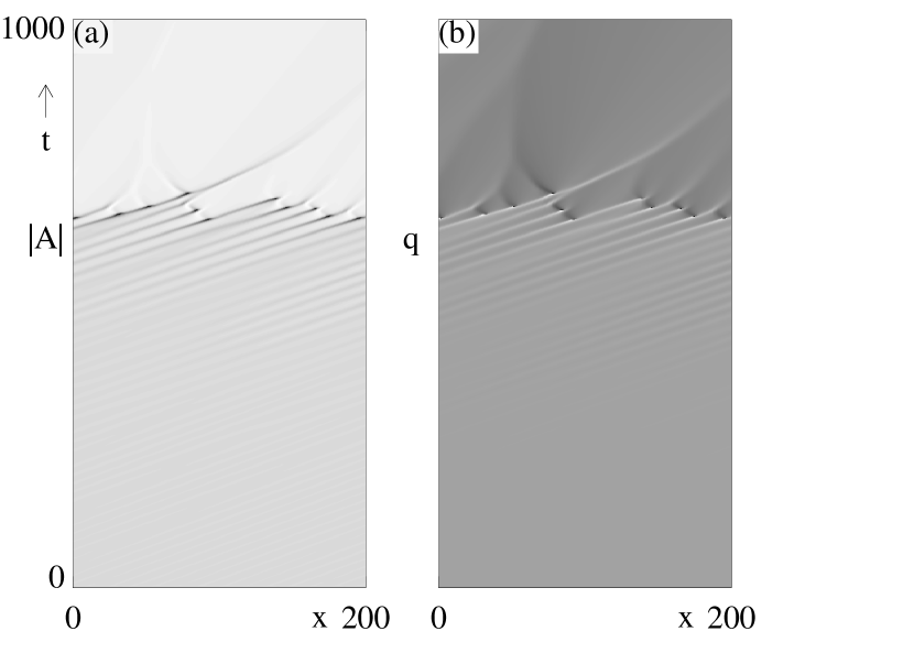
Figure 3: Space-time plot of the evolution of the Benjamin Feir instability of a plane wave with initial wavenumber $q_{pw}=0.41$, for $c_{1}=c_{3}=0.8$ in a system with periodic boundaries and size 400; only part of the system is shown. The slow growth of a transient MAW can be observed, and since this MAW is “beyond the saddle-node”, it does not saturate but develops defects. This dynamics is the one depicted by arrow D in Fig. 1, and is very reminiscent of defect formation observed in hydrothermal waves (see Fig. 6 of [25]) and rotating Rayleigh-Bénard convection [26].

Starting from stable MAWs, a number of MAW properties may be probed.

1. When the period of MAWs is altered (by periodic local heating or sudden changes of $\varepsilon$) and increased, two possible types of dynamics may occur. When $c_{1}$ and $c_{3}$ are relatively small, the MAW may become prone to the splitting instability [2, 3], and new peaks in $q$ may be generated between the old ones, effectively decreasing the period $P$. When $c_{1}$ and $c_{3}$ are larger, the effect of increasing $P$ may be to cross the saddle-node bifurcation, and defects will then occur [2]. Since the occurrence of this saddle-node appears to be a crucial ingredient for the understanding of the transition from phase to defect chaos, this would be extremely interesting to see.

2. When the period of MAWs is decreased, the interaction instability may kick in, which breaks the periodicity of the MAWs [2].

3. When the winding number of MAWs becomes sufficiently small, MAWs become unstable (see [3, 23]). In principle, the effective wavenumber changes when $\varepsilon$ is varied, but at the same time the effective period $P$ changes also. Therefore, a change of $\varepsilon$ can either lead to MAW instabilities or defect-formation, depending on which instability is closest. If it is possible to manipulate $P$ by local periodic heating, then changing this period according to the changes made in $\varepsilon$ may be a way to change the effective value of $\nu$.

4. While it is difficult to say anything general about the MAW profiles, it is known that the minimal value of $|A|$ and the extremum of $|q|$ both grow as a function of the period. In fact, near the SN they decrease ($|A|$) and increase ($|q|$) sharply, which could be used to estimate if this bifurcation is close by.

3.1.2 Transient MAWs.

When the plane wave is stable but close to its Eckhaus instability, perturbations of this plane wave will decay rather slowly, and transient MAWs can be formed. By measuring the decay time as a function of the wavenumber, one can make an estimate for the proximity of the Eckhaus instability (see [25]).

When a plane wave becomes unstable due to the Eckhaus instability, the first stages are characterized by the development of periodic modulations. This period is determined by the most unstable wavenumber of the Eckhaus instability. When these modulations do not grow out to phase chaos or MAWs, but instead grow without bound, defects will eventually occur; a typical example is shown in Fig. 3. The transient MAWs are, as usual, characterized by their period $P$ and winding-number $\nu$ (which is equal to the wavenumber of the initial wave). Defect formation is then expected to occur when, for the current values of $c_{1}$ and $c_{3}$, $P$ and $\nu$ lie beyond the appropriate saddle-node bifurcation [2, 3]. When $P$ and $\nu$ are relatively close to the saddle-node, the formation of defects can be rather slow, and transient holes can be observed; these are clearly incoherent (see [25, 27] for possible experimental realizations of this).

3.2 Incoherent Homoclon dynamics

Homoclons are never linearly stable; over the course of time, they either slowly decay or grow out to form a phase-slip [4, 5]. It will be assumed that their dynamics is studied in a background of linearly stable plane waves. In earlier studies it was found that the instability of the Homoclons is due to a single “core”-mode, and its unstable eigenvalue is the one which changes sign at the saddle node bifurcation where MAWs and Homoclons merge and disappear [2, 3].

This single weakly unstable eigenmode is reflected in the dynamics of the Homoclons. Many sufficiently localized wavenumber-blobs will be attracted to the 1D unstable manifold of the Homoclon; subsequently they then evolve along this manifold, in either the “decay” or the “phase-slip” direction. One can loosely think of the homoclinic holes as unstable equilibria, or separatrices, between plane waves and phase-slips [4, 5].

These properties can be probed as follows: Suppose one has a stable plane wave, and locally perturbs it by generating a twist in the phase field of $A$. When this twist is small, the linear stability of the plane waves will govern the dynamics and such a perturbation will decay diffusively (downward pointing arrow A and B of Fig. 1). However, when it is strong enough, and the initial conditions “passes through the Homoclon separatrix”, the twist will grow out to form a defect (upward pointing arrows A of Fig. 1). When tuning the initial twist so as to be in between the decay and defect scenario, one can obtain a Homoclon that exists for an arbitrarily long time (In practice, noise may limit this time.). The non-trivial prediction is that, since there is only one unstable eigenmode, one only needs a one-parameter family of initial conditions to “hit” the unstable Homoclon solution. This situation was explored already in [4] in the intermittent regime, but it is also possible to generate homoclons in the “laminar” CGLE regime dominated by stable plane waves (see Fig. 4). In addition, the profiles of incoherent homoclons evolve, within good approximation along a one-dimensionally family; if one takes many snapshots of incoherent homoclons and orders them by their extremal phase-gradient $q_{ex}$, profiles with the same $q_{ex}$ should look fairly similar (see [4] for a theoretical check of this). These properties open up the possibility for a number of experiments that follow below.

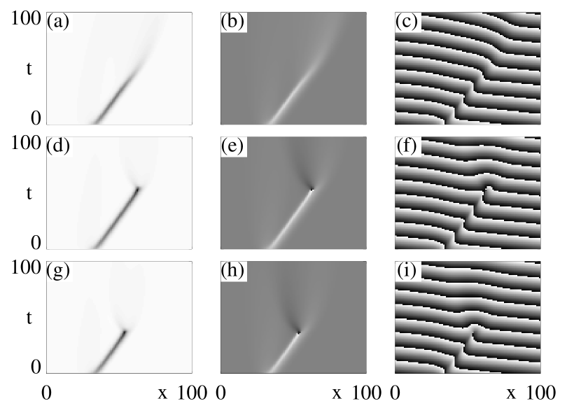
Figure 4: Incoherent Homoclons for $c_{1}=c_{3}=0.5$. The first column shows the evolution of $|A|$ (white: $|A|=1$) while the second column shows the evolution of $q$ (grey: $q=0$, light: $q>0$). The third column shows the evolution of the phase of an artificially created “fast” field: for that $A$ has been multiplied with a plane wave solution. (a,b,c) Initial phase-twist just below Homoclon equilibrium. (d,e,f) Initial phase-twist just above Homoclon equilibrium. (g,h,j) Initial phase-twist further above Homoclon equilibrium; the only difference to d,e,f is the shorter lifetime of the incoherent Homoclon here due to a different initial condition.

3.2.1 Creating transient Homoclons

As discussed above, transient Homoclons can be generated in a large range of coefficient space, provided one can locally perturb the system sufficiently. A possible experimental protocol would be as follows.

• Generate a stable plane wave, and find a way to locally perturb this wave. As discussed above, thermal systems could be perturbed by local heating and many systems could be perturbed by mechanical means. Whatever method one uses, one would expect to be able to tune the strength of the perturbation.

• Clearly, for small enough perturbations no defects will be formed, but instead the perturbation will drift with the group velocity and decay diffusively. The question is: can one make a large enough perturbation that grows out to a defect? This is the necessary ingredient; and this is where clever experiments will be the best way to find out what perturbations are most successful. From a theoretical point of view, it is known that perturbations that “twist” the phase-field are most effective. I would imagine that the effect of local heating is a local increase of the effective value of $\varepsilon$, and the resulting change in time and spatial scales will certainly lead to the generation of phase-twists. If these are done in the middle of the system, likely two pairs of twists are generated (at either side of the perturbed region), so it may be advantageous to perform the perturbations at the edge.

• Denote the control parameter that controls the strength of the perturbation as $V$. If, defects are formed for $V=V_{2}$, while for $V=V_{1}$ the perturbation decays, the experimental protocol is then to repeat this experiment for a number of values between $V_{1}$ and $V_{2}$ to obtain a critical value $V_{c}$ between decay and defect generation. Approaching this value, the theory predicts that transient Homoclons of longer and longer lifetimes occur, and that their lifetime diverges as $-\lambda^{-1}ln(|V-V_{c}|)$ [5], where $\lambda$ is the unstable eigenvalue of the Homoclon [5].

• The theory predicts that the tuning of a single parameter is sufficient to come arbitrarily close to a coherent Homoclon, i.e., if one has two control parameters, say $V$ and $W$, than there should be a continuous curve in $V,W$ space where the Homoclon lifetime diverges.

• Finally, if one is able to tune the wavenumber of the plane wave that the Homoclon propagates into, this also can be used as a parameter. This property was explored in [5] in the regime where the coefficients $c_{1}$ and $c_{3}$ are such that the defects generated by Homoclons lead to the birth of new homoclons and periodic hole-defect states occur. Even when this is not the case, i.e., in the “laminar” regime, the lifetime of a Homoclon can still be controlled by the asymptotic wavenumber.

3.2.2 Spontaneous incoherent Homoclon generation

There are a number of states in which incoherent Homoclons are generated. First there is the hole-defect chaos that occurs in a part of the so-called spatial-temporal intermittent regime of the CGLE [4, 5, 19]; as far as I am aware, this state has not yet been experimentally observed. In experiments it is often possible to have sources between left and right traveling waves, and in that case a sufficient lowering of $\varepsilon$ leads to the creation of unstable sources that send out irregular phase-twists that can lead to transient Homoclons [29].

In both of these states one may study the $a$ and $q$ profiles of snapshots of the holes, and see if they indeed can be ordered as a one parameter family as is the case for the CGLE [4]. In addition, when following $q_{ex}$ as a function of time for a hole, the time derivative $\dot{q}_{ex}$ should be a function of $q_{ex}$ only [5]; this should be revealed in scatter-plots of $\dot{q}_{ex}$ versus $q_{ex}$. Finally it should be remarked that the late stages of defect formation in hole-defect dynamics also is expected to show some universal features; for more see [5].

3.3 Nozaki-Bekki holes

I will not spend much time on the incoherent dynamics of Nozaki-Bekki holes since there is already a very large body of literature available [7, 10, 11]. There is a potentially large range of dynamical behaviors possible for NB holes, due to either dynamical or structural instabilities. When one would observe dynamical NB holes in an experiment, it may be interesting to measure the time-scales as a function of $\varepsilon$. For a CGLE-like structure, these should scale as $\varepsilon^{-1}$, but if the dynamics is due to the structural instability one may expect a larger exponent here, since the deviation from the CGLE can also be expected to scale with $\varepsilon$; on the other hand, when NB holes are dynamically unstable, the structural instability may be irrelevant.

3.4 Identification of local structures

What sort of states can be expected to be seen in experiments? In the light of the experimental data available and our discussion of the properties of the various coherent structures, three possibilities seem most common: (i): Stable MAWs (either in small systems or for high winding-number) [21, 25, 32] (ii): Transient MAWs that evolve to defects [25, 26] (iii) Holes that may be Homoclons or NB Holes. Since cases (i) and (ii) have been discussed already in the sections above, only the distinction between Homoclons and NB holes will be addressed.

When one observes coherent holes, this situation appears simple: When the two wavenumbers of the adjacent waves are equal, they may be Homoclons, when the are different, they may be NB holes. The problem is that in realistic situations, both wavenumbers always will be different, due to noise etc; as can be expected due to the structural and dynamical instabilities of these structures, typically incoherent holes are observed. For incoherent structures, one cannot take a single snapshot and compare this to the profile of either Homoclons or NB holes. Also, the wavenumbers at both sides of an incoherent Homoclon are, due to the combination of an evolving core and phase conservation, not equal (see [4, 5]).

There is, however, a clear difference between incoherent Homoclons and NB holes, which manifests itself in the direction of the full nonlinear group-velocity of the adjacent waves. I would even like to go so far as to propose this as a definition:
In the frame moving with the incoherent hole, incoherent NB holes send out waves, while incoherent Homoclons have one incoming and one outgoing wave.
Needless to say, checks on the direction of the group-velocity are also useful for coherent holes.

An important consequence of this is that two incoherent NB holes cannot sit immediately next to each other, but need to be separated by a so-called sink [24] (unless they have very different propagation velocities). This feature can be used when it is difficult to measure the group velocity, or when this velocity becomes close to the propagation velocities of the holes (which is the case for small $\varepsilon$, where the group velocity becomes close to the linear group velocity $s_{d}$; see appendix A).

I will now briefly discuss some earlier experimental work in which holes are observed; for a more general overview of earlier experimental work, the reader is referred to [11, 15]. In [12], convection of a low Prandtl number fluid in an annular container is studied. Heated wires embedded in the walls of this container yield horizontal temperature gradients which result in a stable two-concentric-roll pattern. These roles become unstable to an oscillatory instability when an additional vertical temperature gradient is imposed, leading to one-dimensional waves that travel along the annulus. For Rayleigh numbers larger than 1.2 $Ra_{crit}$, these waves are stable, and the authors focus on the case that $Ra=1.1Ra_{crit}$, when the homogeneous wave becomes unstable and strong but slowly varying amplitude and wavenumber modulations develop along the pattern. The authors conclude that these modulations presumably are not described by (coupled) CGLEs; the modulation does, however, yield a local area of relative large wavenumber in which holes are generated.

These holes propagate for a finite amount of time, and in many cases lead to the formation of defects. To quote the authors: “We observe the spontaneous creation of traveling dips in a traveling wave pattern. They appear in a region of low amplitude and propagate through it. They change their depth and the value of the phase jump at their core as they move”. While it is difficult to make definitive statements, it may very well be that the holes are formed in a manner similar to that shown in Fig. 3, i.e., due to the instability of a wave; the authors in fact claim this in their conclusion. At the point of writing of this paper, only NB holes were known and the authors speculate that the structures they observe are NB holes, but I doubt that: now that we know that beside NB holes, there are also Homoclons and “ghost” states such as shown in Fig. 3, the question what sort of holes where observed in this experiment is, in my opinion, open.

In [13], oscillatory Rayleigh-Bénard convection in a low Prandtl number fluid (argon gas) is studied. The state of ’coupled oscillators’ that the authors observe may become chaotic, in which cases holes occur (see their Fig. 6). The holes are “characterized by a strong amplitude dip and a phase jump localized at their cores.” They have a finite lifetime and terminate in defects. “The slower they move, the deeper the amplitude dip”. The incoherent motion of the holes, their evolution to defects and the fact that a defect can generate a pair of holes with opposite phasejump (see Fig. 6 of [13]) all are strongly reminiscent of the dynamics of incoherent Homoclons. As before, when this paper was written, only NB holes were known and so naturally the authors speculate that their holes are of this form, but it seems fair to say that the situation is unclear; in fact, the dynamics shown in their Fig. 6 could at least as well be due to homoclinic type holes, also because strong evidence for significantly different wavenumbers at both sides of the holes is absent [33].

More recently, a careful study of holes occurring in hydrothermal waves in a laterally heated fluid layer was carried out. The system consisted of a rectangular container of length 25cm and width 2cm, in which left and right traveling of typical wavelegnth 5mm occured. The coefficients $v_{gr}$, $\xi_{0}$ and $\tau_{0}$ where all measured, and $\varepsilon$ was at a value of 0.19. The dynamical state that occurs then (see Fig. 2 of [14]) is that of an unstable source which separates left and right traveling waves; this source sends out perturbations that develop into (incoherent) holes. The authors claim that these holes are of NB type. By measuring the profile of such hole (in particular their left and right wavenumber and the value of the amplitude minimum), and comparing these to values know from the NB family, they estimate that $c_{1}\approx-1.5$ and $c_{3}\approx 0.4$; the authors claim that similar values of $c_{1}$ and $c_{3}$ were obtained for a number of different holes send out by the unstable source. Unfortunately, no independent measurements of the coefficients $c_{1}$ and $c_{3}$ could be extracted for the hydrothermal waves. Using the values of the coefficients quoted by the authors, I studied the behavior of the (coupled) CGLEs here, using the values of the coefficients quoted by the authors (including a rescaled group-velocity of 1.7), and found indeed an unstable source that sends out hole-like perturbations (see [16] for an explanation of the instability of the source). In the simulations these holes are quite incoherent, and it is difficult to see whether they are homoclinic or heteroclinic.

I have no acces to the raw data, and the evidence for NB holes presented is impressive. Nevertheless, there are some puzzling aspects to this experiment. For the values of coefficients and wavenumbers quoted, NB-holes are quite unstable; I found in simulations of a single CGLE that even the generation of transient unstable NB holes is difficult to achieve for generic initial conditions; I do not know of any mechanism that would generate unstable NB holes, and it is therefore surprising, but not impossible, that these holes are seen in experiment! Another thing that worries me is the size of the holes, and their ill separation. The snapshot of a NB hole that the authors show in their Fig. 4 has an extension of roughly 50mm on the scale of their spacetime diagram Fig. 2, and so I would have expected to see clear differences in wavenumbers and sinks in the spacetime-diagram. But this diagram shows the occurrence of holes that are close together (distance approximately 10-20 mm), without any indication of a sink in between that would separate them if they would be NB holes. Also, NB-holes are sources, so they should send out waves; again, I don’t see any evidence for this.

An alternative, but possibly less satisfying interpretation of the data goes as follows. First note that the total time shown in the spacetime plot is quite short also (105 sec, while $\tau_{0}/\varepsilon=8$ sec [14]), and that all propagation is completely dominated by the linear group velocity. The holes, when they are just send out from the source, form defects, and the pre-defect holes appear reminiscent of (transient) Homoclons; their dynamics is quite fast and so the wavenumbers to the left and right should be substantially different; in fact they seem so incoherent, that detailed comparison to either NB or homoclinic holes seems fairly hopeless. As far as I understand, the holes studied by the authors are the ones formed after these defects have occurred. If one now takes the single CGLE and studies defect formation for the coefficients quoted by the authors, one finds (for example by taking an initial wave of high wavenumber ($0.6$)), that after the last defect was formed, a transient state persisted for a few timeunits that is characterzized by a dip of $|A|$, and two wavenumber “blobs” (that come from the decaying defect); one could interpret these as patches of waves with different wavenumbers to the left and right of this dip. When one switches on the group velocity, such structures are swept away, and could look similar to traveling holes. These structures decays than fairly rapidly (of the other of 10-20 time units in CGLE, which would be 80-160sec in the experiment), but are, in my opinion, not related to any coherent or incoherent hole state. Note that the occurrence of short timescales is inherent in small-$\varepsilon$ experiments in finite systems; either very large systems or periodic boundary conditions may make more detailed comparison of the holes send out by unstable sources in hydrothermal waves possible in the future, and I’m looking forward to see what would come out of such experiments!

Finally, in [34], the dynamics of holes and the formation of defects is studied in the Taylor-Dean system. In this system a traveling wave with negative phase diffusion occurs, and phase gradients concentrate and lead to defects (in related work, these authors observed stable MAWs [32]). The dynamics depicted in Fig. 10 and 11 of [34] suggest that transient Homoclon-like structures play a role here. Finally, in a recent study of sources and holes in a heated wire convection experiment [29], the dynamics of holes send out by unstable sources is studied. The temporal evolution of the profile of the holes shows properties reminiscent of that of Homoclons; nevertheless some questions remain open.

Notwithstanding all these indications, in my opinion neither NB holes or Homoclons have been observed unambiguously yet. Experiments in which the coefficients of the amplitude equation are measured independently and compared to the profile and evolution of holes, or precise comparison of group-velocities and propagation velocities of holes may well show (unstable) NB holes. Similarly, experiments in which initial phasetwists can be shown to lead to either long or short lived holes (similar to Fig. 4) may yield more definite experimental evidence for Homoclons.

4 Conclusion and Outlook

In this paper I hope to have given a broad and easy accessible introduction to the dynamics of MAWs and Homoclons, and some clarification on the Homoclon/NB hole issue. Hopefully some of the suggestions made above will inspire new experiments. Maybe this is the right moment to give a personal perspective on why one could still be interested in complex dynamics in one-dimensional systems.

There is no overall applicable principle or method to describe non-equilibrium systems, but a large subclass is characterized by a combination of nonlinearity and spatial extend. While in general it is not clear how to go from the tools developed for low dimensional dynamical systems to an effective description for systems with many degrees of freedom, the coherent/incoherent structures framework sketched in this paper seems to be able to form such bridge in the case of the CGLE.

Possibly the greatest advantage of studying one-dimensional systems is that their time evolution can be captured in two-dimensional space-time plots, which allow the development of intuition for these systems. Without these, the discovery of most of the Homoclon and MAW dynamical properties would have been much more difficult.

The uncovered mechanisms by which an unstable wave can give rise to MAWs, or, beyond the saddle-node, to defects, and the existence of Homoclons that act as separatrices between defect free and defect developing states, are not trivial. I have some hope that these mechanisms may prove to be more general, and therefore it will be extremely interesting to see what happens in experiments.

Finally, when $\varepsilon$ is increased sufficiently, new mechanisms will start to play a role in the experiments, and the interplay between these and the “low $\varepsilon$” dynamics described here will be interesting. The range of experiments, although potentially large, over which the CGLE dynamics is applicable has not yet been sufficiently mapped out: let us hope that more will be known in the next few years.

4.1 Acknowledgments

The work to uncover the phase gradient structures and their behavior was carried out in collaboration with Markus Baer, Lutz Brusch, Martin Howard, Mads Ipsen, Alessandro Torcini and Martin Zimmerman and I thank them for an interesting journey. In addition, numerous discussions with Igor Aranson, Tomas Bohr, Hugues Chaté, Francois Daviaud, Lorenz Kramer, Wim van Saarloos and Willem van de Water are gratefully acknowledged.

Appendix A Coefficients of the CGLE in the labframe

The spacetime diagrams one obtains in experimental situations cannot be directly compared with the predictions from the CGLE, since the simple form of the CGLE (1) is only obtained after a number of rescalings and coordinate transforms that I will discuss here. It is convenient to introduce first the dimensionless parameter $\varepsilon$ that measures the distance of the controlparameter to threshold [15]. At threshold ($\varepsilon\!=\!0$), the mode with dimensional wavenumber $q_{c}$ and frequency $\omega_{c}$ (nonzero) becomes unstable.

The central observation underlying the amplitude equation approach is that for small but finite positive values of $\varepsilon$ one expects a band of wavenumbers of width $\propto\sqrt{\varepsilon}$ to play a role. Hence close to threshold one expects that a physical field $u$ can be written as the product of a slowly varying amplitude $A$ with the critical mode: $u(x_{d},t_{d})\propto\exp(i(q_{c}x_{d}-\omega_{c}t_{d}))A(x,t)+c.c.$ [15], where $x$ and $t$ denote the slow non-dimensionalized space and time coordinates. After substituting this ansatz into the underlying physical equations of motion (assuming that they are known) and performing a rather tedious expansion up to third order in $\varepsilon$ [15, 35, 36], one then obtains the appropriate amplitude equations: the cubic complex Ginzburg Landau equation. In its full dimensional form, which is most appropriate for highlighting the problems one may encounter when comparing to real data, the equation reads:

$$\tau_{0}(\frac{\partial A_{d}}{\partial t_{d}}-s_{d}\frac{\partial A_{d}}{\partial x_{d}})=\varepsilon(1+ic_{0})A_{d}+\xi_{0}^{2}(1+ic_{1})\frac{\partial^{2}A_{d}}{\partial x_{d}^{2}}-g_{0}(1-ic_{3})|A_{d}|^{2}A_{d}~{}.$$ (8)

To compare experimental data to the CGLE for $A_{d}$ (Eq. (8)), one has to eliminate the fast scales corresponding to the critical mode, and to do so one proceeds as follows.

• Perform a Laplace transform on the experimental spacetime data set $u$ to obtain a complex valued field $U$ as a function of the labframe coordinates $x_{d}$ and $t_{d}$ [29].

• Find the onset for pattern formation, and measure the critical wavenumber $q_{c}$ and frequency $\omega_{c}$, i.e., characterize the wave obtained for $\varepsilon$ as close to zero as possible.

• Demodulate the field $U$ to obtain the dimensional field $A_{d}$, by writing $A_{d}\!=\!U\exp(i(q_{c}x_{d}-\omega_{c}t_{d}))$ (assuming one wave with positive phase-velocity).

One now has obtained a complex field $A_{d}$ that is described by the dimensional amplitude equation Eq. (8).

For a theoretical analysis, most of the coefficients occurring in Eq. (8) can be scaled out. The coefficients $\tau_{0}$ and $\xi_{0}$ give typical temporal and spatial scales to the equation as given by the dispersion relation for plane waves. Going to the so-called dimensionless slow scales $x$ and $t$, which are defined as $x:=\sqrt{\varepsilon}\xi_{0}^{-1}x_{d}$ and $t:=\varepsilon\tau_{0}^{-1}t_{d}$ sets the coefficients $\xi_{0},\tau_{0}$ and the linear growthrate $\varepsilon$ equal to 1. By writing $A_{d}=g_{0}^{-1/2}\exp{(ic_{0}t)}A$, the coefficients $g_{0}$ and $c_{0}$ are scaled to 1 and 0 respectively, and the non-dimensionalized form of $A$ is obtained. The linear, dimensional group velocity $s_{d}$ can be removed by going to a comoving frame, but this only makes sense when the system has periodic boundary conditions; for a finite system with fixed boundaries, the value of $s_{d}$ does play an important role. Assuming that one can go to the comoving frame, the CGLE in its simple form (1) is obtained.

A.1 Measuring the CGLE coefficients

The coefficients $\tau_{0},s_{d},c_{0},\xi_{0}^{2},c_{1},g_{0}$ and $c_{3}$ can in principle be calculated from the underlying equations of motion [15, 35, 36]. For many experimental situations, however, such calculations are not available or can only be done in certain approximations; for some systems the equations of motion or boundary conditions are not even known in enough detail to allow such calculations. Since the scale and even qualitative character of the dynamics depends on these coefficients, their knowledge is essential. The task of measuring these coefficients appears rather nightmarish at first sight, but as I hope to show below, may in fact not be terribly complicated. For recent examples of experimental determinations of these coefficients see [14, 29, 26].

A.1.1 Homogeneous solutions and dispersion relation

When one searches for homogeneous but possibly growing or decaying plane wave solutions of Eq. (8) of the form $a(t_{d})\exp(i(q_{d}x_{x}-\omega_{d}t_{d}))$ one obtains a complex valued equation, of which the real part reads:

$$\partial a/\partial t_{d}=\varepsilon-\xi_{0}^{2}q_{d}^{2}-g_{0}a^{2}~{}.\\$$ (9)

When $a$ is time-independent, the real and imaginary part of this equation are:

$$\tau_{0}\omega = \varepsilon c_{0}-\tau_{0}s_{d}q_{d}+\xi_{0}^{2}c_{1}q^{2}-g_{0}c_{3}a^{2}$$ (10)

$$0 = \varepsilon-\xi_{0}^{2}q_{d}^{2}-g_{0}a^{2}~{}.$$ (11)

Finally, when one restricts oneself to plane wave solutions, where Eq. (11) is satisfied, Eq. (10) becomes the “nonlinear” dispersion relation for plane waves:

$$\tau_{0}\omega=\varepsilon(c_{0}-c_{3})-\tau_{0}s_{d}q_{d}+\xi_{0}^{2}(c_{1}+c_{3})q^{2}$$ (12)

These equations will be the basis for the experiments described below.

A.1.2 Quenches of $\varepsilon$

The coefficients $\tau_{0}$, $c_{0}$ and $c_{3}$ can be obtained by performing experiments where $\varepsilon$ is suddenly changed from one value to another. The simplest case is when initially the system is below threshold $(\varepsilon<0)$ and then suddenly the control parameter is changed to a positive value $\varepsilon_{i}$. A nonlinear plane wave state will start to grow then. Assuming that one is in the linear regime, that this growing wave is spatially homogeneous and has wavenumber $q_{d}=0$, one finds from Eqs. (9) that $a\propto\exp(\tau_{0}\varepsilon t_{d})$. Denote the time interval during which the wave goes from 10% to 50% of its final strength by $t_{i}$. Plotting $\varepsilon$ versus $1/t_{i}$ then should show a linear relationship with a slope give by $\tau_{0}$.

During such quenches one can measure the frequency $\omega$, both when the wave just starts to grow and when it is fully developed. From Eq. (10) one finds that, for $q_{d}=0$, an infinitesimal wave has frequency $\varepsilon/\tau_{0}c_{0}$, while a fully developed wave has frequency (Eq. (12) $\varepsilon/\tau_{0}(c_{0}-c_{3})$. So from these two measurements $c_{0}$ and $c_{3}$ can be determined.

Of course, the assumption that the waves are homogeneous and have wavenumber $q_{d}=0$ may not always be satisfied. However, it is known that for small but positive $\varepsilon$ the band of allowed wavenumbers shrinks $\propto\sqrt{\varepsilon}$, while the spatial modulational scales similarly. Therefore, when the growth-rate is rapidly changed from $\varepsilon_{1}$ to $\varepsilon_{2}$ and back a number of times, where $\varepsilon_{1}$ is close to zero while $\varepsilon_{2}$ is not, one expects to indeed have a homogeneous plane wave of wavenumber very close to zero. Then one can use Eq. (9) which, for $q_{d}=0$, becomes $\partial a/\partial t_{d}=\varepsilon-g_{0}a^{2}$ to get a full numerical prediction of $a$ as a function of time. Comparing this full solution to the experimentally obtained curves for $a(t_{d})$, both for the “up” as well as for the “down” quench for a range of values of $\varepsilon_{1}$ and $\varepsilon_{2}$ then gives accurate estimates for both $g_{0}$ and $\tau_{0}$.

A.1.3 Propagation of linear perturbations

Suppose one has generated a stable plane wave and locally perturbs this wave. Then, as discussed above, the temporal evolution of this perturbation will be a combination of slow diffusion and advection with group velocity $\partial\omega_{d}/\partial q_{d}$. For waves of wavenumber $q_{d}=0$, this group velocity is the linear group velocity $s_{d}$, and for more general waves one finds by differentiating the nonlinear dispersion relation that the nonlinear groupvelocity is $s_{d}+2\xi_{0}^{2}q_{d}(c_{1}+c_{3})/\tau_{0}$. For a measurement of $s_{d}$ it is therefore easiest to make $q_{d}$ equal to zero, which can, for example, be done by varying $\varepsilon$ up and down as described above. It should be noted that while small perturbations may be difficult to observe in noisy snapshots of the system, they often become quite clear in space-time plots of the raw data $u$.

When the perturbations are relatively smooth, such that $\partial a/\partial t$ is small, a comparison of the instantaneous amplitude $a$ and local wavenumber $q$ leads to another condition on the coefficients of the CGLE. From Eq. (10) one finds $g_{0}|A|^{2}=\varepsilon-\xi_{0}^{2}q^{2}$. Plotting $|A|^{2}/\varepsilon$ versus $q^{2}/\varepsilon$ one expects a linear relation. For $q^{2}\downarrow 0$ the value of $|A|^{2}/\varepsilon$ approaches $g_{0}$, while the slope of the curve will be equal to $\xi_{0}^{2}/g_{0}$.

A.1.4 Fronts

When $\varepsilon$ is suddenly increased from below to above threshold, details of the noise and the initial conditions determine the details of the growth of the nonlinear state. Above it has been assumed that one has a homogeneous state, but when a localized perturbation is applied just before such a change of $\varepsilon$ occurs, it is possible to create a pair of fronts that propagate into the unstable $a=0$ state, and leave a nonlinear state in their wake. The point is that for large times the velocity of the front and the wavenumber of the nonlinear state are selected and can be calculated from an essentially linear analysis [15, 24]. These velocities are $s_{d}\pm 2\xi_{0}/\tau_{0}\sqrt{\varepsilon(1+c_{1}^{2})}$, and the wavenumber of the plane wave they leave behind is $q_{c}+\xi_{0}^{-1}\sqrt{\varepsilon/(1+c_{1}^{2})}$ [24]. It should be noted that the velocity and waveumber only relax to their asymptotic values as $1/t$, so it is hard to avoid making some errors here.

A.1.5 Eckhaus instability

As discussed in the section on MAWs, one can manipulate the effective wavenumber of a plane wave state by changes of $\varepsilon$. At some point, when the effective value of $q$ becomes too large, one will encounter the Eckhaus instability, which for general $\varepsilon$ is given by $q^{2}<\varepsilon\xi_{0}^{-2}\frac{(1-c_{1}c_{3})}{3-c_{1}c_{3}+2c_{3}^{2}}$ [20]. This could be used as an independent check on the coefficients.

Appendix B Coherent structure ODEs

The coherent structure ODEs obtained when the ansatz Eq. (4) is substituted into the CGLE can be written in a number of forms and for a number of different dependent variables. All useful representations will have $a$ and $q:=\partial_{\xi}\phi$ as variables, but there are broadly speaking two choices; either $b:=\partial_{\xi}a$ or $\kappa:=(\partial_{\xi}a)/a$ [24, 4, 2, 3]. The latter representation is particularly useful if one wants to study structures, such as fronts, that asymptotically decay to $A=0$. $\kappa$ then measures the exponential decay of the profile to the zero state. Using this latter notation the set of coupled ordinary differential equations (ODE’s) becomes

$$\partial_{\xi}a = \kappa a~{},$$ (13)

$$\partial_{\xi}z = -z^{2}+\frac{1}{1+ic_{1}}\left[-1-i\omega+(1-ic_{3})a^{2}-vz\right]~{},$$ (14)

where the complex quantity $z$ is equal to $\kappa+iq$, which is also equal to $\partial_{\xi}\ln(A)$. Equation (14) is equivalent to two real valued equations, so (13,14) can also be seen as a 3D real-valued dynamical system [24]. Note that since the CGLE is a complex, second order equation one may have expected to find 4 coupled ODEs, but they can be reduced to 3 equations using the phase symmetry of the CGLE.

For completeness note that another ansatz is frequently encountered in the literature: $A=a(\xi)\exp(i(qx-\omega t))\exp(i\phi(\xi))$. This may be convenient if one wants to split off an explicit wavenumber $q$ and require that $\partial_{\xi}\phi$ goes to zero for $\xi\rightarrow\pm\infty$. It is easy to show that this ansatz is equivalent to ansatz (4), and so the apparent three free parameters of this ansatz can be reduced to two [11].

References

- [1] K. Nozaki and N. Bekki, Jour. Phys. Soc. Jap. 53, 1581 (1984).
- [2] L. Brusch, M. G. Zimmermann, M. van Hecke, M. Bär, A. Torcini, Phys. Rev. Lett. 85, 86 (2000); L. Brusch, A. Torcini, M. van Hecke, M. G. Zimmermann and M. Bär, Physica D 160, 127 (2001).
- [3] L. Brusch, A. Torcini and M. Bär, preprint (2001); L. Brusch, “Complex patterns in extended oscillatory systems”, PhD thesis, Dresden (2001).
- [4] M. van Hecke, Phys. Rev. Lett. 80, 1896 (1998).
- [5] M. van Hecke, M. Howard, Phys. Rev. Lett. 86, 2018 (2001); M. Howard and M. van Hecke, in preparation.
- [6] M. Ipsen and M. van Hecke, Physica D 160, 103 (2001).
- [7] S. Popp, O. Stiller, I. Aranson, A. Weber and L. Kramer, Phys Rev Lett 70, 3880 (1993); S. Popp, O. Stiller, I. Aranson and L. Kramer, Physica D 84, 398 (1995); O. Stiller, S. Popp and L. Kramer, Physica D 84, 424 (1995) ; O. Stiller, S. Popp, I. Aranson and L. Kramer, Physica D 87, 361 (1995);
- [8] H. Chaté, Physica D 86, 238 (1995).
- [9] I. S. Aronson, L. Aronson, L. Kramer and A. Weber, Phys. Rev. A 46, R2992 (1992); G. Huber, P. Ahlstroem and T. Bohr, Phys. Rev. Lett. 69, 2380 (1992).
- [10] H. Sakaguchi, Prog. Theor. Phys. 85, 417 (1991); H. Sakaguchi, Prog. Theor. Phys. 86, 7 (1991); H. Chaté and P. Manneville, Phys. Lett. A 171, 183 (1992).
- [11] L. Kramer and I. Aranson, Rev. Mod. Phys. 74, 99 (2002).
- [12] J. Lega, B. Janiaud, S, Jucquois and V. Croquette, Phys. Rev. A 45, 5596 (1992).
- [13] J.-M. Flesselles, V. Croquette and S. Jucquois, Phys. Rev. Lett. 72, 2871 (1994).
- [14] J. Burguete, H. Chaté, F. Daviaud and N. Mukolobwiez, Phys. Rev. Lett. 82, 352 (1999).
- [15] M. C. Cross, P. C. Hohenberg, Pattern formation outside of equilibrium, Rev. Mod. Phys. 65, 851 (1993).
- [16] M. van Hecke, C. Storm, W. van Saarloos, Physica D 134 (1999) 1 and references therein
- [17] P. Coullet, T. Frisch and F. Plaza, Physica D 62, 75 (1993); E. Knobloch and J. Deluca, Nonlinearity 3, 975 (1990); C. Martel and J. M. Vega, Nonlinearity 11, 105 (1998); H. Riecke and L. Kramer, Physica D 137, 124 (2000).
- [18] B. I. Shraiman, A. Pumir, W. van Saarloos, P. C. Hohenberg, H. Chaté, M. Holen, Physica D 57, 241 (1992).
- [19] H. Chaté, Nonlinearity 7 185 (1994).
- [20] T. B. Bejamin and J. E. Feir, J. Fluid Mech. 27, 417 (1967).
- [21] B. Janiaud, A. Pumir, D. Bensimon, V. Croquette, H. Richter and L. Kramer, Physica D 55, 269 (1992).
- [22] L. Kramer and W. Zimmermann, Physica D 16, 221 (1985).
- [23] R. Montagne, E. Hernandez-Garcia and M. San-Miguel, Phys. Rev. Lett. 77, 267 (1996); A. Torcini, Phys. Rev. Lett. 77 1047 (1996).
- [24] W. van Saarloos, P. C. Hohenberg, Physica D 56, 303 (1992); Physica D 69, 209 (1993) (errata).
- [25] N. Mukolobwiez, A. Chiffaudel and F. Daviaud, Phys. Rev. Lett. 80, 4661 (1998).
- [26] Y. M. Liu and R. E Ecke, Phys. Rev. E 59, 4091 (1999).
- [27] Y. Liu and R. E. Ecke, Phys. Rev. Lett. 78, 4391 (1997).
- [28] J. M. Vince and M. Dubois, Physica D 102, 93 (1997).
- [29] L. Pastur, M.-T. Westra, W. van de Water, M. van Hecke, C. Storm and W. van Saarloos, arXiv cond-mat/0111234; L. Pastur, M.-T. Westra and W. van de Water, Physica D, this issue.
- [30] N. Garnier and A. Chiffaudel, Phys Rev. Lett. 86, 75 (2001); idem, this issue of Phys. D.
- [31] V. Croquette and H. Williams, Phys. Rev. A 39, 2765 (1989).
- [32] P. Bot, O. Cadot and I. Mutabazi, Phys. Rev. E 58, 3089 (1998).
- [33] J.-M. Flesselles, private communications (1999).
- [34] P. Bot and I Mutabazi, Eur. Phys. J. B. 13, 141 (2000).
- [35] E. Y. Kuo and M. C. Cross, Phys. Rev. E 47, R2245 (1993).
- [36] M. van Hecke and W. van Saarloos, Phys. Rev. E. 55, R1259 (1997); M. van Hecke, ’The amplitude description of nonlinear patterns’, PhD thesis, Leiden University (1996).