Coarsening process in one-dimensional surface growth models

Abstract

Surface growth models may give rise to instabilities with mound formation whose tipical linear size $L$ increases in time (coarsening process). In one dimensional systems coarsening is generally driven by an attractive interaction between domain walls or kinks. This picture applies to growth models for which the largest surface slope remains constant in time (corresponding to model B of dynamics): coarsening is known to be logarithmic in the absence of noise ($L(t)\sim\ln t$) and to follow a power law ($L(t)\sim t^{1/3}$) when noise is present. If surface slope increases indefinitely, the deterministic equation looks like a modified Cahn-Hilliard equation: here we study the late stages of coarsening through a linear stability analysis of the stationary periodic configurations and through a direct numerical integration. Analytical and numerical results agree with regard to the conclusion that steepening of mounds makes deterministic coarsening faster : if $\alpha$ is the exponent describing the steepening of the maximal slope $M$ of mounds ($M^{\alpha}\sim L$) we find that $L(t)\sim t^{n}$: $n$ is equal to ${1\over 4}$ for $1\leq\alpha\leq 2$ and it decreases from ${1\over 4}$ to ${1\over 5}$ for $\alpha\geq 2$, according to $n=\alpha/(5\alpha-2)$. On the other side, the numerical solution of the corresponding stochastic equation clearly shows that in the presence of shot noise steepening of mounds makes coarsening slower than in model B: $L(t)\sim t^{1/4}$, irrespectively of $\alpha$. Finally, the presence of a symmetry breaking term is shown not to modify the coarsening law of model $\alpha=1$, both in the absence and in the presence of noise.

1 Introduction

In real systems surface growth occurs on two-dimensional (2d) substrates and therefore its modelization in one dimension (1d) is in general an oversimplification, mainly justified by the possibility to have a deeper understanding of the dynamical evolution of the system. In some cases the surface indeed maintains a 1d profile, for example when the relaxation of a grooved surface is studied grooves . This is not true when the surface undergoes kinetic roughening or a growth instability followed by a phase separation: in both cases, noise makes the resulting morphology 2d even if the initial one is 1d. The dynamical evolution of a vicinal surface is another possible application of 1d models. In fact, if atomic steps move in phase PRL_Saito , step motion is described by a one-dimensional growth equation.

In this paper we are interested in a growing surface that undergoes a kinetic instability. The origin of such an instability is related to an additional barrier that diffusing adatoms must overcome to descend step edges (the so-called Ehrlich-Schwoebel (ES) barrier KE ; libroJV ). Even in the presence of stabilizing mechanisms, at sufficiently large scales the ES effect can be the dominant one and the flat surface becomes unstable against small deformations. In a first linear regime, a structure with a well-defined wavelength emerges and its amplitude increases in time. At a later stage, nonlinearities come into play and the mound structure typically –but not unavoidably PRL_Saito – coarsens.

This simplified picture reminds spinodal decomposition and coarsening that take place during phase separation. Surface growth instability and phase separation do have strong similarities and they can indeed be equivalent in 1d review . However, they are definitely different in two dimensions coarsening2d .

Generally speaking, phase separation has different properties in one and two dimensions. We mention here two of them revBray : (i) In 2d, coarsening is driven by the tension of domain walls while in 1d it is due to interaction between walls. (ii) Noise is generally irrelevant in 2d, while it modifies the coarsening law in 1d (except in the presence of long-range interactions).

The class of models that we study in one dimension is of interest in two respects. First, since the slope is assumed to increase indefinitely, it is not possible to speak of domain walls between different phases. Second, being the interaction long ranged, noise may happen to be irrelevant for the coarsening law in 1d: this occurs for some of the models studied here.

In the next Section we give a short introduction to the continuum equations that are encountered in one-dimensional models of conserved surface growth. A more detailed analysis can be found in recent review papers review ; revJK . In Section 3 we recall a few theoretical approaches to one-dimensional coarsening and in Section 4 we apply the linear stability analysis to our class of deterministic $\alpha$-models. Its results are confirmed by numerics. The problem of coarsening in the presence of noise is addressed directly via stochastic numerical integration in Section 5. In Section 6 we examine the effect of a symmetry breaking term, while the discussion of the results and our conclusions are presented in the final Section.

2 Models for unstable surface growth

In the Introduction we have already mentioned the ES barriers as a source of the kinetic instability. In fact, it is well-known VilJdP that an asymmetry in the sticking coefficients of an adatom to a step produces a slope-dependent current $j_{\hbox{\tiny ES}}(m)$; $h(x,t)$ and $m=\partial_{x}h$ are the local height and slope of the surface. It is more convenient to use the variable $z(x,t)=h(x,t)-\bar{h}$, where $\bar{h}=F_{0}t$ is the average height, instead of $h(x,t)$ ($F_{0}$ being the intensity of the flux). In this way the evolution equation $\partial_{t}h=F_{0}-\partial_{x}j$ simply writes $\partial_{t}z=-\partial_{x}j$ while the definition of the slope $m=\partial_{x}h=\partial_{x}z$ is unaffected.

For symmetry reasons, $j_{\hbox{\tiny ES}}$ is an odd function of $m$. Therefore we expect that $j_{\hbox{\tiny ES}}\simeq\nu m$ at small slopes, as confirmed by a more rigorous analysis review . The asymmetry in the sticking coefficients is generally due to the additional energy barrier hindering the adatom from descending a step. This gives rise to an up-hill current $j_{\hbox{\tiny ES}}\simeq\nu m$ with a positive coefficient $\nu$. This implies that $j_{\hbox{\tiny ES}}$ has a destabilizing character, as easily revealed by the solution of the linear differential equation $\partial_{t}z=-\partial_{x}j_{\hbox{\tiny ES}}=-\nu\partial_{x}^{2}z(x,t)$ : $z(x,t)=z_{0}\cos(qx)e^{\omega_{q}t}$, with $\omega_{q}=\nu q^{2}$.

In a continuum model, where the lattice constant $a$ goes to zero, the following expression for $j_{\hbox{\tiny ES}}$ can be used:

$$j_{\hbox{\tiny ES}}={\nu m\over 1+\ell_{\hbox{\tiny D}}^{2}m^{2}}~{}~{}~{}~{}~{}~{}\hbox{model 1}~{}.$$ (1)

If a discrete model with square symmetry is used, we expect $j_{\hbox{\tiny ES}}$ to vanish for $m=m_{0}=1/a$ . We can therefore define the model:

$$j_{\hbox{\tiny ES}}=\nu m(1-m^{2}/m_{0}^{2})~{}~{}~{}\hbox{model 0}$$ (2)

However, other mechanisms can produce a slope-dependent current: short-range step-adatom interaction KE ; AF , post-deposition transient mobility and downward funneling Evans . The first mechanism may be either stabilizing or not, depending on the sign of the step-adatom interaction while the other (non-thermal) mechanisms are typically stabilizing, i.e. they contribute with a negative term $-\nu^{\prime}m$ to $j_{\hbox{\tiny ES}}$. Because of that, either the ES current acquires a zero at finite slope (from model 1 we pass to model 0) or there is a change in the value $m_{0}$ at which $j_{\hbox{\tiny ES}}$ vanishes.

Finally, in a previous paper JPA we have generalized Eq. (1) to a class of models ($\alpha$-models) characterized by different asymptotic behaviors for $m\to\infty$:

$$j_{\hbox{\tiny ES}}={\nu m\over(1+\ell_{\hbox{\tiny D}}^{2}m^{2})^{\alpha}}~{}~{}~{}~{}~{}~{}\hbox{model }\alpha~{}(\geq 1)~{}.$$ (3)

In the Introduction we also mentioned possible stabilizing mechanisms. The simplest expression for a stabilizing current is the so-called Mullins term that in its linearized form reads $j_{\hbox{\tiny M}}=K\partial_{x}^{2}m$. Its origin may be either thermodynamic (relaxation through surface diffusion Mullins ) or kinetic (fluctuations in the nucleation process of new islands PV ; Nato_Rodi ). A stabilizing current gives a negative contribution to $\omega_{q}$. Starting from the equation $\partial_{t}z=-\partial_{x}(j_{\hbox{\tiny ES}}+j_{\hbox{\tiny M}})$ it is easily found that $\omega_{q}=\nu q^{2}-Kq^{4}$. A flat surface is thereby linearly unstable against fluctuations of wavelength larger than $\lambda_{c}=2\pi\sqrt{K/\nu}$.

Both currents $j_{\hbox{\tiny ES}}$ and $j_{\hbox{\tiny M}}$ change sign if $x\to-x$ or $z\to-z$: the growth process cannot break the former symmetry but it does break the latter. It has been shown VilJdP ; PV that such symmetry breaking term (intrinsically nonlinear) has the form $j_{\hbox{\tiny SB}}=\partial_{x}A(m^{2})$, where $A\sim m^{2}$ at small slopes and $A\sim-1/m^{2}$ at large ones. Its presence is strictly related to the breaking of the detailed balance principle Racz and therefore to the non-equilibrium character of the growth process.

It has been proven kinks that $j_{\hbox{\tiny SB}}$ does not modify the coarsening law of model 0: the effects of $j_{\hbox{\tiny SB}}$ on model 1 will be considered in Section 6.

We conclude this Section by writing down explicitly the class of growth equations that are analyzed in the paper:

$$\partial_{t}z(x,t)=-\partial_{x}j(x,t)+\eta(x,t)$$ (4)

$$j(x,t)=\left\{\begin{array}[]{lr}\partial_{x}^{2}m+{m\over(1+m^{2})^{\alpha}}&\hbox{model }\alpha\cr\partial_{x}^{2}m+m(1-m^{2})&\hbox{model }0\end{array}\right.$$ (5)

$$\langle\eta(x,t)\rangle=0~{}~{}~{}\langle\eta(x,t)\eta(x^{\prime},t^{\prime})\rangle=\tilde{F}_{0}\delta(x-x^{\prime})\delta(t-t^{\prime})$$ (6)

Eq. (4) is the evolution equation of the local height $z(x,t)$ for a conserved growth process in the presence of the shot noise $\eta(x,t)$; Eqs. (5) give the currents for the $\alpha$-models and model 0, once that $x,t,z$ have been rescaled in order to get an adimensional equation; Eq. (6) gives the spectral properties of the noise, whose strength $\tilde{F}_{0}=F_{0}a\ell^{2}/\sqrt{\nu K}$ is the only parameter appearing in the problem: $F_{0}$ is the intensity of the flux, $a$ is the lattice constant, $\ell$ is the diffusione length $\ell_{\hbox{\tiny D}}$ for $\alpha$-models (Eqs. (1,3)) or the inverse of the constant slope $m_{0}$ for model 0 (Eq. (2)), $\nu$ and $K$ are the prefactors of $j_{\hbox{\tiny ES}}$ and $j_{\hbox{\tiny M}}$, respectively.

3 Theoretical approaches to coarsening

In this Section we review two theoretical methods that have been used to study the coarsening process in model 0. The first method uses the property that the current $j_{\hbox{\tiny ES}}$ vanishes at a finite slope $m_{0}$. Although it can not be used for $\alpha$-models, for completeness and clarity we discuss it in Section 3.1. The second method consists in a linear stability analysis of the stationary configurations. It is a very general method and it is discussed in Section 3.2. In the context of phase separation processes it was introduced by Langer Langer to study model 0 and its solution is proposed in Section 4.1. Its application to $\alpha$-models is carried out in Section 4.2.

3.1 Kink dynamics

Model 0 and $\alpha$-models have the same linear behaviour, but they strongly differ in the nonlinear regime: in model 0 the slope increases up to the maximal value $m_{0}=\pm 1$ while in $\alpha$-models it grows indefinitely.

For model 0, the surface profile corresponding to a constant value $m_{0}=1$ (i.e. to a vicinal surface with unitary slope) is stable note2 , but it can not be attained starting from a flat surface because the average slope must remain constant. Still, we can consider the stationary configuration $m_{+}(x)$ ($j(m_{+}(x))\equiv 0$) corresponding to a limiting slope $\pm m_{0}$ for $x\to\mp\infty$. That profile is called ‘mound’ in the $z$-space and ‘kink’ or ‘domain wall’ in the space of the order parameter $m$, where it has the form $m_{+}(x)=\tanh(x/\sqrt{2})$.

During the coarsening process of model 0 a typical surface profile is just an alternating sequence of kinks ($m=m_{+}(x)$) and antikinks ($m=m_{-}(x)=-m_{+}(x)$), whose average distance $L(t)$ increases with time because of the annihilation process between pairs of neighbouring kink-antikink. In the absence of noise the dynamics of kinks is governed by their attractive interaction that decays exponentially with the distance, since $|m_{\pm}(x)|\simeq 1-2\exp(-\sqrt{2}|x|)$ for $|x|\gg 1$. Such a weak interaction determines a very slow coarsening: $L(t)\sim\ln t$ giap ; Langer .

In the presence of noise the picture is different because of the induced fluctuations on the kink positions. If there were no constraint induced by the conservation of the order parameter, kinks would simply perform a random walk and therefore would travel a distance $L$ in a typical time $L^{2}$, giving a coarsening exponent $n=1/2$ ($L(t)\sim\sqrt{t}$). In a growth process, where a conservation law does exist, kink trajectories are not independent and the coarsening slows down: $n=1/3$. This exponent is more easily understood in a spin picture CKS , where the conservation of the order parameter (the magnetization) implies that the system evolves through spin-exchange processes (Kawasaki dynamics).

If we now turn to $\alpha$-models, we recognize that the kink picture is not applicable because the unstable current $j_{\hbox{\tiny ES}}$ vanishes for infinite slope only.

3.2 Linear stability analysis of stationary configurations

We now discuss the linear stability analysis of the stationary configurations. They are determined by the condition $\partial_{t}z(x,t)\equiv 0$, i.e. the current must be a constant: $j\equiv c$. The net current $c$ is related to the average slope of the surface: we are interested in a high symmetry surface and therefore we set $c=0$.

The equation $j=0$ is formally equal to the Newton’s equation for a particle of unitary mass, where the slope $m$ plays the role of the particle position and $x$ the role of time:

$$\partial_{x}^{2}m(x)+j_{\hbox{\tiny ES}}(m)=0~{}.$$ (7)

The fictitious particle feels the force $-j_{\hbox{\tiny ES}}(m)$, i.e. it moves in the potential $V_{\hbox{\tiny ES}}(m)=\int^{m}dsj_{\hbox{\tiny ES}}(s)$. Different models give qualitatively different potentials (see Fig. 1):

$$V_{\hbox{\tiny ES}}(m) = m^{2}/2-m^{4}/4~{}~{}~{}~{}~{}~{}~{}~{}~{}~{}~{}~{}~{}\hbox{model 0}$$ (8)

$$V_{\hbox{\tiny ES}}(m) = (1/2)\ln(1+m^{2})~{}~{}~{}~{}~{}~{}~{}~{}~{}~{}\hbox{model 1}$$ (9)

$$V_{\hbox{\tiny ES}}(m) = -(1+m^{2})^{1-\alpha}/[2(\alpha-1)]~{}\hbox{model }\alpha>1$$ (10)

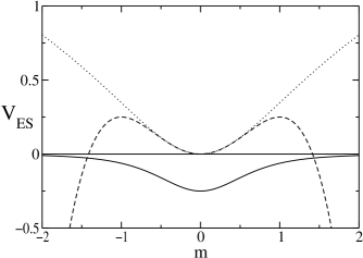
Figure 1: Profiles of the different potentials $V_{\hbox{\tiny ES}}$. From top to bottom: Model 1 (dotted line), Eq. (9); Model 0 (dashed line), Eq. (8); Model $\alpha=3$ (full line), Eq. (10).

Stationary configurations therefore correspond to the periodic oscillations of the particle around the minimum of $V_{\hbox{\tiny ES}}$ in $m=0$. We label the stationary configurations $m_{\hbox{\tiny 2L}}(x)$ through their period $2L$. What about the limit $L\to\infty\;$? For model 0 it corresponds to the kink-solution: $m_{\hbox{\tiny$\infty$}}(x)=m_{+}(x)\to\pm 1$ when $x\to\pm\infty$. For model 1, the energy of the particle diverges when the period $L$ increases and the limiting configuration $m_{\hbox{\tiny$\infty$}}(x)$ does not exist. It does exist for $\alpha>1$ and it corresponds to the well defined problem of a particle of zero energy moving in the potential (10): it starts at $m=-\infty$ and arrives at $m=+\infty$ after an infinite time.

We start by considering small deviations $\psi$ from the periodic profile: $m(x,t)=m_{\hbox{\tiny 2L}}(x)+\psi(x,t)$. Since $j_{\hbox{\tiny ES}}(m_{\hbox{\tiny 2L}}+\psi)=j_{\hbox{\tiny ES}}(m_{\hbox{\tiny 2L}})+j_{\hbox{\tiny ES}}^{\prime}(m_{\hbox{\tiny 2L}})\psi+{\cal O}(\psi^{2})$, we obtain that the linearized evolution equation for $\psi(x,t)$ is

$$\partial_{t}\psi=\partial_{x}^{2}\left[-\psi^{\prime\prime}(x,t)-j_{\hbox{\tiny ES}}^{\prime}(m_{\hbox{\tiny 2L}}(x))\psi\right]$$ (11)

and therefore the time dependence of $\psi$ is: $\psi(x,t)=\phi(x)\cdot$ $\exp(-\epsilon t)$. Replacing the expression of $\psi$ in terms of $\phi$ into Eq. (11), we find that the stability is determined by the spectrum of the following operator:

$$(-\partial_{x}^{2})\left[-\phi^{\prime\prime}(x)+U_{\hbox{\tiny L}}(x)\phi\right]\equiv D_{x}\hat{H}\phi(x)=\epsilon\phi~{},$$ (12)

where $D_{x}\equiv-\partial_{x}^{2}$ and $\hat{H}\equiv-\partial_{x}^{2}+U_{\hbox{\tiny L}}(x)$ is a single-particle Schroedinger operator corresponding to the periodic potential $U_{\hbox{\tiny L}}(x)\equiv-j_{\hbox{\tiny ES}}^{\prime}(m_{\hbox{\tiny 2L}}(x))$, of period $L$:

$$U_{\hbox{\tiny L}}(x+L) = -j_{\hbox{\tiny ES}}^{\prime}(m_{\hbox{\tiny 2L}}(x+L))$$ (13)

$$= -j_{\hbox{\tiny ES}}^{\prime}(-m_{\hbox{\tiny 2L}}(x))=U_{\hbox{\tiny L}}(x)~{}.$$

In one dimension coarsening is due to the unstable character of the periodic stationary configurations, i.e. to the existence of negative eigenvalues in the energy spectrum nota1 . Because of the periodic character of the operator $D_{x}\hat{H}$, eigenvalues are grouped into bands.

Our evolution equation for $m(x,t)$ is $\partial_{t}m=D_{x}j$ where the current $j$ (see Eq. (5)) can be derived from a pseudo free energy ${\cal F}$:

$$j=-{\delta{\cal F}\over\delta m}~{}~{}~{}~{}~{}~{}~{}{\cal F}=\int dx[\hbox{${1\over 2}$}(\partial_{x}m)^{2}-V_{\hbox{\tiny ES}}(m)]$$ (14)

For model 0 the potential $-V_{\hbox{\tiny ES}}(m)$ has the standard double well shape and $m(x,t)$ evolves accordingly to the Cahn-Hilliard equation; in the presence of conserved noise we obtain the so-called model B of dynamics HH . If $D_{x}$ is replaced by the identity operator, the order parameter is no longer conserved and its evolution equation is $\partial_{t}m=j$, which is equivalent for model 0 to the time dependent Ginzburg Landau equation, or –in the presence of nonconserved noise– to model A of dynamics HH . We use the notations $\tilde{\epsilon},\tilde{\phi}$ for the spectrum of the operator $D_{x}\hat{H}$ and $\epsilon,\phi$ for the Hamiltonian operator $\hat{H}$.

Let us start with few general statements on the lowest part of the spectrum. Translational invariance implies that $\epsilon=0$ is always an eigenvalue of the operator $\hat{H}$ (and therefore $\tilde{\epsilon}=0$ is an eigenvalue of $D_{x}\hat{H}$ as well) and it corresponds to the eigenfunction $\phi(x)=\tilde{\phi}(x)=m_{\hbox{\tiny 2L}}^{\prime}(x)$. To prove it let us use the definition of $m_{\hbox{\tiny 2L}}(x)$ as solution of the differential equation (7) and take its derivative:

$$m_{\hbox{\tiny 2L}}^{\prime\prime\prime}(x)+j_{\hbox{\tiny ES}}^{\prime}(m_{\hbox{\tiny 2L}})m_{\hbox{\tiny 2L}}^{\prime}(x)=0~{}.$$ (15)

Since $U_{\hbox{\tiny L}}(x)=-j_{\hbox{\tiny ES}}^{\prime}(m_{\hbox{\tiny 2L}}(x))$ we just have

$$-\partial^{2}_{x}(m_{\hbox{\tiny 2L}}^{\prime}(x))+U_{\hbox{\tiny L}}(x)(m_{\hbox{\tiny 2L}}^{\prime}(x))\equiv\hat{H}m_{\hbox{\tiny 2L}}^{\prime}(x)=0~{}.$$ (16)

Therefore the operators $\hat{H}$ and $D_{x}\hat{H}$ have a zero energy eigenvalue and the corresponding eigenfunction $m_{\hbox{\tiny 2L}}^{\prime}(x)$ has period $\lambda=2L$ (i.e. it corresponds to the wavevector $q=\pi/L$ in the Bloch representation).

We can now recognize the importance of the limit $m_{\hbox{\tiny$\infty$}}(x)$. If $m_{\hbox{\tiny$\infty$}}(x)$ exists, for $L\to\infty$ the periodic potential $U_{\hbox{\tiny L}}(x)$ becomes a single well potential $U_{\hbox{\tiny$\infty$}}(x)$. In this limit $m_{\hbox{\tiny 2L}}(x)$ is a monotonic function $m_{+}(x)$ (the kink solution, for model 0). Therefore $\tilde{\phi}_{1}(x)=\phi_{1}(x)\equiv m_{+}^{\prime}(x)$ has no node and it represents the ground state for the single well problem. For finite $L$ we have a periodic potential and the energy level $\epsilon_{1}=\tilde{\epsilon}_{1}=0$ gives rise to the lowest band of the spectrum. The ground state $\epsilon_{\hbox{\tiny GS}}(L)$ of the operator $\hat{H}$ corresponds to $q=0$ and must therefore have a negative energy, implying that $\hat{H}$ has negative eigenvalues. The relation $\tilde{\epsilon}_{\hbox{\tiny GS}}=\tilde{\epsilon}(q=0)$ is no longer valid for the conserved model, but Langer Langer has shown that negative eigenvalues $\epsilon$ of $\hat{H}$ may be put in correspondance to negative eigenvalues $\tilde{\epsilon}$ of $D_{x}\hat{H}$ (see Section 4.1).

Since an unstable mode increases exponentially with the factor $\exp(|\epsilon|t)$, the knowledge of the $L$ dependence of the ground state energy allows to find the deterministic coarsening law $L(t)$ via the relations $|\epsilon_{\hbox{\tiny GS}}(L)|\sim 1/t$ (nonconserved model) and $|\tilde{\epsilon}_{\hbox{\tiny GS}}(L)|\sim 1/t$ (conserved model).

4 Deterministic coarsening

In Fig. 2 we plot the single well potentials $U_{\hbox{\tiny$\infty$}}(x)$ for model 0 (dashed line) and for model $\alpha=3$ (full line), the latter being representative of all the class of $\alpha$-models. Since, as already explained, $\epsilon_{1}=0$ is the ground state energy for the single well, completely different behaviours are expected in the two cases.

For model 0 (see Section 4.1), $U_{\hbox{\tiny$\infty$}}(x)$ approaches 2 at large $x$: therefore the wavefunction $\phi_{1}(x)$ decays exponentially at large distances and energy shifts due to the tunneling between wells at finite distance $L$ are expected to be exponentially small. This property is the counterpart of the exponentially vanishing interaction between kinks, discussed in Section 3.1.

For $\alpha$-models (see Section 4.2), $U_{\hbox{\tiny$\infty$}}(|x|=\infty)=0=\epsilon_{1}$ and the considerations developed for model 0 do not apply.

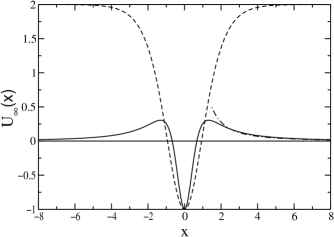
Figure 2: The single well potential $U_{\hbox{\tiny$\infty$}}(x)$ for model 0 (dashed line) and for model $\alpha=3$ (full line). At large $x$ the former approaches 2, while the latter vanishes as $U_{\hbox{\tiny$\infty$}}(x)=a/x^{2}$, with $a=10/9$ (dashed-dotted line, see formula (25)).

4.1 Model 0

For model 0 the kink-solution is $m_{\hbox{\tiny$\infty$}}(x)=\tanh(x/\sqrt{2})$, the single well potential is (see the dashed line in Fig. 2)

$$U_{\hbox{\tiny$\infty$}}(x)=-1+3m_{\hbox{\tiny$\infty$}}^{2}(x)=-1+3\tanh^{2}(x/\sqrt{2})$$ (17)

and the corresponding ground state wavefunction is $\phi_{1}(x)=m_{\hbox{\tiny$\infty$}}^{\prime}(x)=\hbox{${1\over\sqrt{2}}$}\sec^{2}(\hbox{${x\over\sqrt{2}}$})$.

For finite $L$, $U_{\hbox{\tiny L}}(x)$ is a collection of wells centred at points $x=0,\pm L,\pm 2L,\dots$ . It is interesting to compare $U_{\hbox{\tiny L}}(x)$ with the periodic potential $U_{\hbox{\tiny L}}^{*}(x)$ obtained as a superposition of the single well potentials $U_{\hbox{\tiny$\infty$}}(x-nL)$:

$$U_{\hbox{\tiny L}}^{*}(x)=U_{\hbox{\tiny$\infty$}}(x)+\sum_{n\neq 0}[U_{\hbox{\tiny$\infty$}}(x-nL)-U_{\hbox{\tiny$\infty$}}(\infty)]~{}.$$ (18)

For model 0, $U_{\hbox{\tiny$\infty$}}(\infty)=2$ and the summation can indeed be limited to the two terms $n=\pm 1$ because the quantity in square brackets is exponentially small. In Fig. 3a we show that $U_{\hbox{\tiny L}}^{*}(x)$ (full line) is an excellent approximation of $U_{\hbox{\tiny L}}(x)$ (circles).

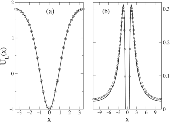
Figure 3: The true periodic potential $U_{\hbox{\tiny L}}(x)$ (empty circles) is compared with the potential $U_{\hbox{\tiny L}}^{*}(x)$ (full line), obtained as a superposition of the single well potentials $U_{\hbox{\tiny$\infty$}}(x-nL)$ (see Eq. (18)). We make this comparison for model 0 (a), where $L\simeq 6.8$, and for model $\alpha=$3 (b), where $L\simeq 22.8$. In both cases we display one period only. $U_{\hbox{\tiny L}}(x)$ is obtained numerically and $U_{\hbox{\tiny L}}^{*}(x)$ is obtained analitically. The superposition principle works well in (a) even for small $L$, while the exact potential for model 3 (see b) is not reproduced by the sum of single well potentials. In order to make more evident the difference between the two potentials, in (b) we focus the plot on the region of positive $U_{\hbox{\tiny L}}(x)$. We remind that $U_{\hbox{\tiny L}}(0)=-1$ for any $\alpha$.

Langer performed a tight-binding-approximation to determine the lowest band of the energy spectrum arising from the ground state $\epsilon_{1}=0$ of the single well. The result Langer is

$$\epsilon(q)\simeq-(1+\cos qL)\exp(-2L)~{},$$ (19)

confirming that $\epsilon(q=\pi/L)=0$, $\epsilon_{\hbox{\tiny GS}}=\epsilon(q=0)$ and that $\epsilon_{\hbox{\tiny GS}}$ decays exponentially with the distance $L$ between wells. The relation $|\epsilon_{\hbox{\tiny GS}}|\sim 1/t$ nota2 implies that coarsening is logarithmically slow: $L(t)\sim\ln t$. This result is valid for the conserved model as well. Langer proved it by means of the variational condition Langer :

$$\tilde{\epsilon}_{\hbox{\tiny GS}}\leq{\epsilon_{\hbox{\tiny GS}}\over(\bar{\phi}_{1},\phi_{1})}$$ (20)

where

$$(\bar{\phi}_{1},\phi_{1})=\int dx\bar{\phi}_{1}^{*}(x)\phi_{1}(x)$$ (21)

is the scalar product between the ground state function $\phi_{1}(x)$ of the Hamiltonian operator and $\bar{\phi}_{1}$ is defined by the relation $D_{x}\bar{\phi}_{1}=\phi_{1}$.

Because of the conservation law, the lowest energy band for the operator $D_{x}\hat{H}$ reads Langer :

$$\epsilon(q)\simeq-\sin^{2}qL\cdot{\exp(-2L)\over L}~{}.$$ (22)

The factor $L$ at denominator is irrelevant and the coarsening law $L(t)\sim\ln t$ is still valid. Eq. (22) also confirms that $\tilde{\epsilon}(q=\pi/L)=0$ and that $\tilde{\epsilon}(q=0)$ is no more the ground state.

4.2 $\alpha$-models

The solution of model 0 by Langer is of great interest because it gives approximate expressions for the lowest energy band, both for the nonconserved (19) and conserved (22) models. The basis of his treatment is the tight-binding-approximation: $\Delta U(x)\equiv U_{\hbox{\tiny L}}^{*}(x)-U_{\hbox{\tiny$\infty$}}(x)$ is taken as a small perturbation of $U_{\hbox{\tiny$\infty$}}(x)$.

In the case of $\alpha$-models, a simpler strategy can be followed JPA by replacing the periodic potential $U_{\hbox{\tiny L}}(x)$ with a double well $U_{\hbox{\tiny 2}}(x)$, obtained by joining rather than superposing $U_{\hbox{\tiny$\infty$}}(x)$ and $U_{\hbox{\tiny$\infty$}}(x-L)$ nota3 . Using this approximation, our analytical results for the coarsening exponent $n(\alpha)$ agre well with the estimate obtained from numerical integration of the growth equations JPA (see the results for the conserved model reported in Fig. 9). In the following we report the general lines of this theoretical approach, and we add a direct numerical confirmation (see Fig. 4).

The single well potential $U_{\hbox{\tiny$\infty$}}(x)$ for the $\alpha$-models (see Fig. 2) decays to zero at large $x$ from positive values. From the relation $U_{\hbox{\tiny$\infty$}}(x)=-j_{\hbox{\tiny ES}}^{\prime}(m_{\hbox{\tiny$\infty$}}(x))$ it is simple to derive that for $m\gg 1$:

$$U_{\hbox{\tiny$\infty$}}(x)\sim{(2\alpha-1)\over m_{\hbox{\tiny$\infty$}}^{2\alpha}(x)}~{}.$$ (23)

The integration of Newton’s equation (7) for zero energy gives the asymptotic result ($x\gg 1$):

$$m_{\hbox{\tiny$\infty$}}^{\alpha}(x)\sim\hbox{${\alpha\over\sqrt{\alpha-1}}$}x~{},$$ (24)

which implies

$$U_{\hbox{\tiny$\infty$}}(x)\sim{(2\alpha-1)(\alpha-1)\over\alpha^{2}}{1\over x^{2}}\equiv{a\over x^{2}}~{}.$$ (25)

Thus the single well potential decays as the inverse of a square law whatever is $\alpha$, but with a prefactor $a$ that increases between $a=0$ for $\alpha=1$ and $a=2$, for $\alpha=\infty$. For $\alpha=3$, $a=\hbox{${10\over 9}$}$ and the corresponding function ${a\over x^{2}}$ is reported in Fig. 2 as the dashed-dotted line, showing the comparison between the asymptotic expansion (25) and the exact expression nota4 .

The solution $\phi_{1}(x)$ of the Schroedinger equation for the single well (let us remind that the ground state has zero energy) therefore decays at large $x$ as a power law JPA : $\phi_{1}(x)\sim|x|^{-\beta}$, with $\beta=(1-\alpha^{-1})$. So, the ground state wavefunction is a bound state for $\beta>\hbox{${1\over 2}$}$ i.e. $\alpha>2$ only.

In Ref. JPA we used the Landau and Lifshitz approach LL for the double-well problem and we extended it to take into account the possibility that the ground state wavefunction for the single well is not a bound state. This happens for $1<\alpha\leq 2$. The main point is that even if $\phi_{1}(x)$ is not a bound state, the ground state $\phi_{2}(x)$ of the double well is bound, because its energy $\epsilon_{2}$ is now strictly negative and so lower than the asymptotic value $U_{2}(\infty)=0$.

Following the above approach we found JPA that

$$|\epsilon_{\hbox{\tiny GS}}(L)|\simeq L^{-\gamma}~{}~{}~{}~{}~{}\gamma=\left\{\begin{tabular}[]{cc}2&$\alpha<2$\cr($3-\hbox{${2\over\alpha}$}$)&$\alpha>2$\end{tabular}\right.~{}.$$ (26)

Once $\gamma$ is known, the coarsening exponent $n$ is just given by $n=1/\gamma$. In Table 1 we summarize the results found in Ref. JPA for the nonconserved and conserved models. For $\alpha=2$ there are logarithmic corrections: $L\sim(t/\ln t)^{n}$.

Table 1: The deterministic coarsening exponent $n$, for the nonconserved ($D_{x}\equiv 1$) and the conserved ($D_{x}\equiv-\partial_{x}^{2}$) models. For $\alpha=2$ there are logarithmic corrections (see JPA ).

	$1<\alpha<2$	$\alpha>2$
nonconserved	${1\over 2}$	${\alpha\over 3\alpha-2}$
conserved	${1\over 4}$	${\alpha\over 5\alpha-2}$

The reason why it has not been possible to treat the periodic potential $U_{\hbox{\tiny L}}(x)$ in a more rigorous way is given in Fig. 3b, where it is clearly shown that the superposition principle does not work for $\alpha$-models: accordingly, the potential $U_{\hbox{\tiny L}}(x)$ can not be approximated as the sum of single-well potentials. Therefore, the application of the tight-binding-approximation is not straightforward because we do not know the explicit expression of the perturbation $\Delta U(x)\equiv U_{\hbox{\tiny L}}(x)-U_{\infty}(x)$. The disagreement between $U_{\hbox{\tiny L}}(x)$ and $U_{\hbox{\tiny L}}^{*}(x)$ might appear at first sight to be unimportant, but if we neglect their difference we obtain wrong results (as we have verified).

However, it is possible to check in a direct way the accuracy of our theory: we solve numerically the quantum mechanical problem to determine the ground state energy $\epsilon_{\hbox{\tiny GS}}(L)$ of the full periodic potential $U_{\hbox{\tiny L}}(x)$ (see Fig. 4 and footnote nota_fig ). The numerical results for the exponent $\gamma$ agree fairly well, at large $L$, with the theoretical predictions $\gamma(3)=2.\bar{3}$ and $\gamma(10)=2.8$. This confirms that our theoretical approach to calculate $\epsilon_{\hbox{\tiny GS}}(L)$ is indeed correct.

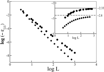
Figure 4: Nonconserved models: on a log-log scale (main) we report the absolute value of the ground state energy $\epsilon_{\hbox{\tiny GS}}(L)$ for the periodic potential $U_{\hbox{\tiny L}}(x)$. Circles refer to model 3 and diamonds to model 10. In the inset we report the local derivatives $d[\log(-\epsilon_{\hbox{\tiny GS}})]/d[\log(L)]$ and the asymptotic values of $\gamma$ that are calculated analytically (see Eq. (26)).

4.3 Numerical analysis

Let us now discuss our numerical results for the deterministic $\alpha$-models. We have numerically integrated the equation of motion (4) with $\eta=0$, starting from an initial profile $z(x,0)=r_{x}$, where $r_{x}$ is a random variable with a flat distribution in the interval $[-0.1,0.1]$.

Tipically, we have followed the dynamical evolution for a total time $t_{\hbox{\tiny MAX}}\sim 400,000-1,600,000$, for a chain length $L_{c}=1024$, with a spatial resolution $\delta x=0.25$ and an integration time step $\tau=0.05$. A few tests have been also performed with a smaller time step $\tau=0.025$ and with longer chains ($L_{c}=2048-4096$), obtaining consistent results. The adopted integration scheme is a time-splitting pseudo-spectral code: more details are reported in App. A.1.

On top of Fig. 5 we display a portion of the surface profile $z(x)$ for the model $\alpha=3$. It appears as made up of constant slope regions separated by domain walls. However, the slope profile $m(x)$ reported in the centre of Fig. 5 does not corroborate this picture: no region of constant slope is clearly visible and the maxima or minima have appreciably different values. The same remark is applicable at later times. On the bottom of Fig. 5 we also display the potential $U(x)=$ $-j_{\hbox{\tiny ES}}^{\prime}(m(x))$ that enters in the analytical solution of the problem (see the previous section). It is therefore reassuring that $U(x)$ looks indeed as a regular sequence of the single well potentials depicted in Fig. 2 as a full line, because it confirms that the surface profile keeps close to a stationary configuration.

Figure 5: Model $\alpha=3$, late stages of coarsening. Top: the surface profile $z(x)$ as obtained via numerical integration. Centre: the slope profile $m(x)=z^{\prime}(x)$. Bottom: the potential $U(x)=-j_{\hbox{\tiny ES}}^{\prime}(m)$. We display only a piece of the total spatial domain.

The next step is to evaluate the characteristic length $L(t)$, corresponding to the average distance between wells. We define the wavevector $p_{c}(t)$ via the relation:

$$p_{c}(t)=\frac{\sum_{p}^{\prime}pS(p,t)}{\sum_{p}^{\prime}S(p,t)}~{},$$ (27)

where $S(p,t)=|{\tilde{z}}(p,t)|^{2}$ is the power spectrum associated to the field $z$ at time $t$ ($\tilde{z}$ being its spatial Fourier transform) and the sum is restricted to the wavevectors $p$ for which $S(p)\geq\delta\cdot S_{\hbox{\tiny M}}$, $S_{\hbox{\tiny M}}$ being the maximum value of the spectrum and $\delta$ some threshold (typical values are $\delta\sim 0.1-0.2$). The characteristic length is then evaluated as $L(t)=2\pi/p_{c}(t)$ and the coarsening exponent $n(\alpha)$ has been obtained by considering the scaling behaviour of $L(t)\sim t^{n}$ in a time interval $10,000<t<400,000-1,600,000$.

As an independent check we have also determined $L$ from the normalized spatial correlation function of the surface profile

$$C(r,t)=\frac{<z(x+r,t)z(x,t)>-<z(x,t)>^{2}}{<z(x,t)^{2}>-<z(x,t)>^{2}}~{},$$ (28)

where the spatial average $<\cdot>$ is performed along the chain. Defining $L$ through the relation

$$C(L,t)=C(0,t)/2$$ (29)

our results are in agreement with the previous ones obtained from the power spectrum in all the considered cases.

The numerically estimated length $L(t)$ is reported in Fig. 6 for $\alpha=1.5,3,10$. The coarsening exponents are $n(1.5)=0.250\pm 0.003$, $n(3)=0.233\pm 0.005$ and $n(10)=0.208\pm 0.002$. These results are consistent with the theoretical estimates for $n(\alpha)$, as summarized in Fig. 9. Their critical discussion is deferred to the final section.

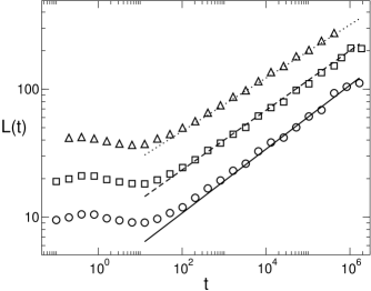
Figure 6: Deterministic coarsening: $L$ vs $t$ in log-log scale for $\alpha=1.5$ ($\circ$), $\alpha=3$ ($\Box$) and $\alpha=10$ ($\triangle$). For presentation purpose the data for $\alpha=3$ and $10$ are shifted by a constant. The lines indicate the best fit to the data for $t>10,000$ and the slopes are equal to 0.250 (—), 0.233 (- - -) and 0.208 ($\cdots$), in agreement with the theoretical prediction (see Table 1).

5 Coarsening with conservative noise

The stochastic equation (4) has been integrated up to a time $t_{\hbox{\tiny MAX}}\sim 800,000$ with $L_{c}=1024$. The results for $L(t)$ and $C(r,t)$ have been obtained by averaging over $N_{c}$ different initial conditions with different noise realizations (tipically $N_{c}=10$). The integration scheme employed in the noisy case is different from the one adopted for the deterministic case and it is described in detail in App. A.2. We have used a noise strength corresponding to a value of $\tilde{F}_{0}$ (see Eq. (6)) equal to 0.05. This is a physically reasonable value because for large ES barriers review , $\tilde{F}_{0}\approx\hbox{${a\over\ell_{\hbox{\tiny D}}}$}$ and $\ell_{\hbox{\tiny D}}$ is typically of the order of a few dozens of lattice constants.

For the noisy case we have defined $L$ only in term of the average correlation function $\overline{C(r,t)}$, where the bar means that average is now performed at each time not only along the chain (see definition  (28)) but also over different noise realizations. A sufficiently good scaling is obtained in the time interval $40,000<t<800,000$ for all the considered values of $\alpha$ ($=1,2,10$).

As a benchmark to verify the validity both of our integration scheme and of our procedure to estimate $n(\alpha)$, we have analyzed model 0. In this case the coarsening exponent is known giap ; Langer to be $n=1/3$. A good agreement between our numerical data and the theoretical prediction is found for $t>40,000$, as shown in Fig. 7.

For the two values of $\alpha$, $\alpha=1$ and $\alpha=10$, we find $n=1/4$. We conclude that, in the presence of shot noise, the coarsening exponent is independent of $\alpha$ and equal to $1/4$. Fig. 7 also suggests the possible existence for model 0 of an intermediate regime (with $L\sim 5-20$) where an effective exponent $n=\hbox{${1\over 4}$}$ is found.

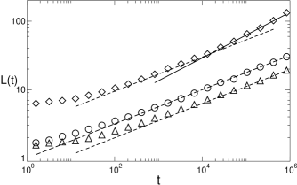
Figure 7: Coarsening in the presence of shot noise: $L$ vs $t$ in log-log scale for model 0 ($\Diamond$) and for $\alpha=1$ ($\triangle$) and $\alpha=10$ ($\circ$). Dashed lines have slope $1/4$ and full line has slope $1/3$.

6 Effects of a symmetry breaking term

In Ref. kinks one of us studied the effect of symmetry breaking on model 0. Since in that model the slope keeps finite with a maximal value equal to one, the detailed expression of the function $A(m^{2})$ ($j_{\hbox{\tiny SB}}=\partial_{x}A$) is not relevant. It was therefore chosen the simplest form, the one valid at small slopes: $A(m^{2})=\lambda^{*}m^{2}$.

On the contrary, for $\alpha$-models the slope can diverge so that the exact expression of $j_{\hbox{\tiny SB}}$ should be used PV :

$$j_{\hbox{\tiny SB}}=-\lambda^{*}\partial_{x}\left({1\over 1+m^{2}}\right)~{}.$$ (30)

We limited ourselves to the physically relevant case $\alpha=1$. We have therefore integrated the following differential equation:

$$\partial_{t}z=-\partial_{x}\left[\partial_{x}^{2}m+{m\over 1+m^{2}}-\lambda^{*}\partial_{x}\left({1\over 1+m^{2}}\right)\right]+\eta$$ (31)

for values of $\lambda^{*}$ varying between 0.1 and 1.

Our results (see Fig. 8) suggest that $j_{\hbox{\tiny SB}}$ is irrelevant for the coarsening law, both for $\eta\equiv 0$ (deterministic case) and for $\eta\neq 0$ (noisy case).

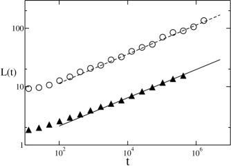
Figure 8: Coarsening for the asymmetric model (Eq. (31) with $\lambda^{*}=1$), in the absence (empty circles) and in the presence (full triangles) of shot noise. Fits have been done for $t>10^{4}$ and give $n=0.25$ without noise (dashed line) and $n=0.24$ with noise (full line). Circles have been shifted by a constant.

7 Discussion and conclusions

In Fig. 9 we have summarized our numerical and theoretical results for the coarsening exponent $n$ ($L\sim t^{n}$). In the absence of noise, our theory (full line) predicts that $n=\hbox{${1\over 4}$}$ for $1<\alpha\leq 2$ and for larger values of $\alpha$ it decreases down to ${1\over 5}$ ($n=1/(5-\hbox{${2\over\alpha}$})$). Numerical results (full circles) agree well with the full fine.

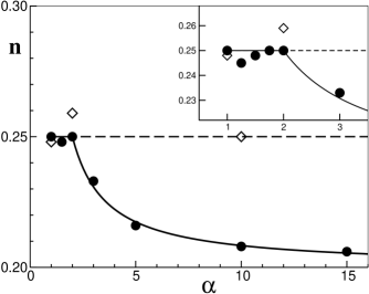
Figure 9: The coarsening exponent $n$ as a function of $\alpha$, for the deterministic models (full circles) and for the stochastic models (open diamonds). In the inset we enlarge the region of small $\alpha$. Full line is the theoretical result in the absence of noise (Table 1) and the dashed line is our ansatz $n=1/4$ for the noisy case.

We are aware of only one analytical paper treating our class of models (Ref. Golub ). The author uses scaling arguments to conclude that, in the absence of noise, $n=1/4$ irrespectively of $\alpha$ and for any dimension $d$ of the substrate. In the following we give a drastically simplified version of the scaling arguments. If $Z,L$ and $M=Z/L$ are respectively the typical height, width and slope of mounds at time $t$, the evolution equation for $z(x,t)$ implies $Z/t\sim j/L$. The current $j$ is made up of the Mullins term, of order $M/L^{2}$ plus the ES current, whose asymptotic expression for large slope is $1/M^{2\alpha-1}$. They vanish in the limit $t\to\infty$ and must be of the same order in ${1\over t}$, which entails the relation $M^{\alpha}\sim L$. If their sum $j$ is supposed to be of the same order as well, the relation $Z/t\sim M/L^{3}$ implies $L(t)\sim t^{1/4}$, i.e. $n=1/4$ for any $\alpha$.

One main drawback of the scaling argument is that the two terms appearing in $j$ are of the same order but their sum is smaller (i.e. of higher order in ${1\over t}$) because of a compensation effect. This is a necessary condition for the stationary configurations to play a role in the coarsening process.

In order to have a direct numerical check of our statement, we have evaluated the quantities $\langle|\partial_{x}j_{\hbox{\tiny M}}|\rangle$, $\langle|\partial_{x}j_{\hbox{\tiny ES}}|\rangle$ and $\langle|\partial_{x}(j_{\hbox{\tiny M}}+j_{\hbox{\tiny ES}})|\rangle$, as a function of time, where $\langle\cdots\rangle$ means, as before, the spatial average. For all the considered values of $\alpha$ ($\alpha=1,3,10$), the result is the same: the ratio $\langle|\partial_{x}j_{\hbox{\tiny M}}|\rangle/\langle|\partial_{x}j_{\hbox{\tiny ES}}|\rangle$ is equal to one, up to higher order terms, and $\langle|\partial_{x}(j_{\hbox{\tiny M}}+j_{\hbox{\tiny ES}})|\rangle/\langle|\partial_{x}j_{\hbox{\tiny M}}|\rangle$ vanishes.

Our numerical results tell even more than that: in fact scaling arguments would suggest that $n$ is strictly smaller than ${1\over 4}$ if $j$ is smaller than $j_{\hbox{\tiny M}}$ and $j_{\hbox{\tiny ES}}$, but for $\alpha\leq 2$ we do find $n=\hbox{${1\over 4}$}$ even if $|j|/|j_{\hbox{\tiny M}}|\simeq|j|/|j_{\hbox{\tiny ES}}|\to 0$.

Model $\alpha=1$ had been previously studied numerically at short times also in Ref. Sander and authors found a value $n\approx 0.22$, independent of the noise strength.

Let us now discuss the results in the presence of noise. Fig. 9 presents with diamonds the numerical results for the stochastic integration of Eq. (4). Our data refer to $\alpha=1,2,10$ and provide a reasonably convincing evidence that in the presence of noise the coarsening exponent remains constant, $n=\hbox{${1\over 4}$}$ (dashed line). The somewhat larger value for $\alpha=2$ may be due to unknown logarithmic corrections.

Authors in Refs. noise1 ; noise2 use qualitative arguments to describe coarsening assisted by noise: they use a ‘single mound’ model and find the coarsening time by requiring that shot noise induces a height fluctuation of the same order of the mound height. In one dimension they find $n=1/(3+\hbox{${2\over\alpha}$})$, where $\alpha$ is defined phenomenologically through the asymptotic relation $M\sim L^{1/\alpha}$ between the typical (or the maximal) slope $M$ and the width $L$ of mounds.

Their prediction for $n(\infty)$ seems to agree with the result $n=\hbox{${1\over 3}$}$ for model 0. This is reasonable because in that model the slope is constant and therefore it can effectively be equivalent to the model $\alpha=\infty$. Actually, if we take the limit $\alpha=\infty$ in Eq. (5), it is straightforward to conclude that the current $j_{\hbox{\tiny ES}}$ vanishes and we obtain the linear equation:

$$\partial_{t}z(x,t)=-\partial_{x}^{4}z(x,t)+\eta(x,t)~{}.$$ (32)

The basic question is whether our class of $\alpha$-models tends –in some sense– to Eq. (32) with increasing $\alpha$. In the absence of noise, the answer is surely negative: indeed, Eq. (32) does not admit stationary periodic solutions that, as discussed above, are crucial for deterministic coarsening.

On the other hand, if noise is present ($\eta\neq 0$), Eq. (32) describes a process of kinetic roughening: the growing surface is characterised by a correlation length $\tilde{\xi}(t)\sim t^{1/\tilde{z}}$, where $\tilde{z}$ is the dynamical critical exponent. In $d=1$ it is well known libroJV that for the quartic linear equation (32), $\tilde{z}=4$. It is reasonable to guess that the stochastic $\alpha$-model does converge to Eq. (32) for $\alpha\to\infty$ and –in the same limit– $n(\alpha)\to\hbox{${1\over\tilde{z}}$}=\hbox{${1\over 4}$}$.

The meaning of a constant value $n=\hbox{${1\over 4}$}$ for any $\alpha$ is simple: in the presence of noise the detailed form of the current $j_{\hbox{\tiny ES}}$ is irrelevant provided that the slope $m$ diverges.

We can now summarize our main results. Without noise, $n=\hbox{${1\over 4}$}$ for $\alpha\leq 2$ and $n=1/(5-\hbox{${2\over\alpha}$})$ for $\alpha>2$. This result has been obtained analytically and it has been confirmed by extensive numerical calculations. It can not be deduced by simple scaling arguments. In the presence of noise our numerical data for $\alpha=1,2,10$ suggest that $n=\hbox{${1\over 4}$}$ irrespectively of $\alpha$. This guess agrees with the well known result $\tilde{\xi}(t)\sim t^{1/4}$, valid for the linear model $\alpha=\infty$. So, steepening of mounds makes coarsening faster without noise and slower with noise.

We believe that the surface profile can not be described as a sequence of mounds with a spatially constant slope $M$ that increases in time (see Fig. 5, centre). This wrong assumption may be the reason why qualitative arguments to determine $n$ do fail.

We have also considered the possible effect of a symmetry breaking term $j_{\hbox{\tiny SB}}$ in the current: it is irrelevant for model 1, as already proved for model 0 kinks .

We conclude the paper by mentioning a different model, whose coarsening properties bear some similarities with our $\alpha$-models. It has been studied by Bray and Rutenberg Bray and it consists in the addition of a long-range attraction between kinks to model 0. If such interaction decays as a power law of the distance ($1/L^{s}$, with $s>1$) the deterministic coarsening exponent is found to be $n=1/(1+s)$. In the presence of conservative noise, this appears to be relevant for $s>2$ and in that case $n=\hbox{${1\over 3}$}$. Some analogies therefore exist with our class of $\alpha$-models, because in both cases the coarsening exponent is a continuously varying function of a parameter ($\alpha$ or $s$), noise may be relevant ($\alpha,s>2$) or not ($1<\alpha,s\leq 2$), and –finally– the stochastic coarsening exponent is constant if noise is relevant.

Appendix A Integration algorithms

Let us rewrite in an explicit way the evolution equation (4) for the field $z(x,t)$:

$$\partial_{t}z(x,t)=-\partial_{x}^{4}z-\partial_{x}\left[\frac{\partial_{x}z}{(1+(\partial_{x}z)^{2})^{\alpha}}\right]+\eta(x,t)\quad,$$ (33)

where $\eta(x,t)$ indicates additive $\delta$-correlated spatio-temporal gaussian noise, i.e.

$$<\eta(x,t)>=0$$ (34)

$$<\eta(x,t)\eta(0,0)>={\tilde{F}}_{0}\delta(x)\delta(t)\quad.$$ (35)

A.1 Deterministic equation

Let us first neglect the noise term: in order to perform the numerical integration of (33) we consider a discrete spatial grid of resolution $\delta x$ and a discrete time evolution with time step $\tau$. The discretized field is written as $z(i,n)$, where the integer indices $i$ and $n$ are the spatial and temporal discrete variables, respectively. Periodic boundary conditions have been considered for the field: $z(i,n)=z(i+I,n)$, where $I$ is the number of sites of the grid ($L_{c}=I\delta x$). The algorithm adopted to integrate (33) is a time-splitting pseudo-spectral code num . In particular, by following rdf Eq.(33) has been rewritten as

$$\partial_{t}z(x,t)=({\cal L}+{\cal N})z(x,t)$$ (36)

where ${\cal L}$ and ${\cal N}$ are two operators defined in the following way: ${\cal L}z=-\partial_{x}^{4}z$ and ${\cal N}z=-\partial_{x}\left[\frac{\partial_{x}z}{(1+(\partial_{x}z)^{2})^{\alpha}}\right]$. As usual for time splitting algorithms, the linear evolution, ruled by the operator ${\cal L}$, is treated independently from the nonlinear one (associated to the operator ${\cal N}$). A complete evolution over an integration time step $\tau$ therefore corresponds to the two successive integration steps:

$$z^{*}(x,t+\tau)=\exp{[{\cal L}\tau]}z(x,t)$$ (37)

and

$$z(x,t+\tau)=\exp{[{\cal N}\tau]}z^{*}(x,t+\tau)$$ (38)

where $z^{*}(x,t)$ is a dummy field.

Let us firstly consider the linear part,

$$\partial_{t}z(x,t)={\cal L}z(x,t)~{}.$$ (39)

Eq.(39) can be easily solved in the Fourier space and the equation of motion for the spatial Fourier transform of the field ${\tilde{z}}(p,t)$ is

$$\partial_{t}{\tilde{z}}(p,t)=-p^{4}{\tilde{z}}\quad.$$ (40)

The time evolution for ${\tilde{z}}$ is simply given by

$${\tilde{z}}^{*}(p,t+\tau)=\exp{[-p^{4}\tau]}{\tilde{z}}(p,t)~{}.$$ (41)

Therefore, in order to integrate Eq.(39), the field should be Fourier transformed in space (${\cal F}$), then multiplied by the propagator reported in Eq.(41) and the outcome of such operation should be finally inverse-Fourier transformed (${\cal F}^{-1}$):

$$z^{*}(x,t+\tau)={\cal F}^{-1}\exp{[-p^{4}\tau]}{\cal F}z(x,t)\,.$$ (42)

The integration of the nonlinear part has been performed by emploing a second-order Adam-Basforth scheme

$$z(x,t+\tau) = z^{*}(x,t+\tau)+$$

$$\frac{\tau}{2}\left[3\,G(z(x,t))-G(z(x,t-\tau))\right]\quad,$$

where $G(z(x,t))=\left\{-\partial_{x}\left[\frac{\partial_{x}z}{(1+(\partial_{x}z)^{2})^{\alpha}}\right]\right\}$. In order to obtain a better precision, the spatial derivatives appearing in $G(z(x,t))$ have been evaluated in the Fourier space.

A.2 Stochastic equation

Let us now consider the noisy problem: in this case the algorithm outlined here above does not guarantee a sufficient precision. Therefore, we have developed a more accurate integration scheme cris that consists as a first step in rewriting the equation of motion (33) in the Fourier space

$$\partial_{t}{\tilde{z}}(p,t)=-p^{4}{\tilde{z}}(p,t)+G_{p}(z,t)+{\tilde{\eta}}(p,t)\,,$$ (44)

where $G_{p}(z,t)$ and ${\tilde{\eta}}(p,t)$ are the Fourier transforms of the nonlinear part and of the noise term appearing in Eq. (33). The amplitudes ${\tilde{\eta}}(p,t)$ of the noise components in the Fourier space are still gaussian $\delta$-correlated stochastic variables with zero average and with a variance ${\cal V}_{p}={\cal F}_{0}/I$ independent of $p$ (white noise). The formal exact solution of (44) is

$${\tilde{z}}(p,t+\tau)=$$ (45)

$${\rm e}^{-p^{4}\tau}\left[{\tilde{z}}(p,t)+\int_{t}^{t+\tau}dt^{\prime}\,{\rm e}^{p^{4}(t^{\prime}-t)}(G_{p}(z,t^{\prime})+{\tilde{\eta}}(p,t^{\prime}))\right]~{}.$$

The problem is now to evaluate the two terms appearing in the integral. The first term has been evaluated adopting a second order Adam-Bashfort scheme. i.e.

$$\int_{t}^{t+\tau}dt^{\prime}\,{\rm e}^{p^{4}(t^{\prime}-t)}G_{p}(z,t^{\prime})=$$ (46)

$$\frac{\tau}{2}\left[3G_{p}(z,t)-{\rm e}^{-p^{4}\tau}G_{p}(z,t-\tau)\right]+{\cal O}(\tau^{3})\,.$$

The treatment of the second term is more delicate, since it is a stochastic integral: we have chosen to evaluate it accordingly to the Ito’s prescription gardiner :

$$\int_{t}^{t+\tau}dt^{\prime}\,{\rm e}^{p^{4}(t^{\prime}-t)}{\tilde{\eta}}(p,t^{\prime})=$$ (47)

$$\left[W_{p}(t+\tau)-W_{p}(t)\right]=\Delta W_{p}(t)\,.$$

Here $W_{p}(t)$ and $\Delta W_{p}(t)$ represent two Wiener processes: in particular we have $\langle\Delta W_{p}\rangle=0$ and $\langle(\Delta W_{p})^{2}\rangle=\tau{\cal V}_{p}$. The complete solution of (44) can be written as

$${\tilde{z}}(p,t+\tau)={\rm e}^{-p^{4}\tau}{\tilde{z}}(p,t)+$$ (48)

$$\frac{3\tau}{2}{\rm e}^{-p^{4}\tau}G_{p}(z,t)-\frac{\tau}{2}{\rm e}^{-2p^{4}\tau}G_{p}(z,t-\tau)+{\rm e}^{-p^{4}\tau}\Delta W_{p}(t)\,.$$

In order to obtain the solution in the real space it is sufficient to inverse-Fourier transform ${\tilde{z}}(p,t+\tau)$.

Due to the spatial and temporal discreteness of the integration scheme, the spatio-temporal noise term $\eta(x,t)$ should be rewritten as $\gamma_{i}^{n}$, where $\gamma$ is a random gaussian variable of zero average and variance

$${\cal V}=\frac{\tau\tilde{F}_{0}}{\delta x}~{},$$ (49)

with

$$<\gamma_{i}^{n}\gamma_{0}^{0}>={\cal V}\delta_{i,0}\delta_{n,0}~{}.$$ (50)

The spatio-temporal discrete gaussian noise, with zero average and standard deviation $\sqrt{\frac{\tau\tilde{F}_{0}}{\delta x}}$ has been numerically generated by employing a Box-Muller algorithm num .

References

- (1) A. Chame, S. Rousset, H.P. Bonzel and J. Villain, Bulg. Chem. Commun. 29, 398 (1996/97) and references therein.
- (2) O. Pierre-Louis, C. Misbah, Y. Saito, J. Krug, P. Politi, Phys. Rev. Lett. 80, 4221 (1998).
- (3) K. Kyuno, G. Ehrlich, Surf. Sci. 383, L766 (1997) and references therein.
- (4) A. Pimpinelli, J. Villain, Physics of crystal growth (Cambridge, Cambridge University Press, 1998).
- (5) P. Politi, G. Grenet, A. Marty , A. Ponchet, J. Villain, Phys. Rep. 324, 271 (2000).
- (6) M. Siegert, Physica A 239, 420 (1997); M. Siegert, Phys. Rev. Lett. 81, 5481 (1998); D. Moldovan, L. Golubovic, Phys. Rev. E 61, 6190 (2000).
- (7) A.J. Bray, Adv. Phys. 43, 357 (1994).
- (8) J. Krug, Adv. Phys. 46, 139 (1997).
- (9) J. Villain, J. de Physique I 1, 19 (1991).
- (10) J.G. Amar, F. Family, Phys. Rev. Lett. 77, 4584 (1996).
- (11) J.W. Evans, Phys. Rev. B 43, 3897 (1991).
- (12) P. Politi, A. Torcini, J. Phys. A: Math. Gen. 33, L77 (2000).
- (13) W.W. Mullins, J. Appl. Phys. 28, 333 (1957).
- (14) P. Politi, J. Villain, Phys. Rev B 54, 5114 (1996).
- (15) P. Politi, J. Villain, in Surface Diffusion: atomistic and collective processes, edited by M.C. Tringides (Plenum Press, New York, 1997) p. 177.
- (16) Z. Rácz, M. Siegert, D. Liu, M. Plischke, Phys. Rev. A 43, 5275 (1991).
- (17) P. Politi, Phys. Rev. E 58, 281 (1998).
- (18) A linear stability analysis of a 1d vicinal surface of constant slope shows that step-flow is stable if .
- (19) K. Kawasaki, T. Ohta, Physica A 116, 573 (1982); K. Kawasali, T. Nagai, Physica A 121, 175 (1983); T. Kawakatsu, T. Munakata, Prog. Theor. Phys. 74, 11 (1985); T. Nagai, K. Kawasaki, Physica A 134, 483 (1986).
- (20) J.S. Langer, Ann. Phys. 65, 53 (1971).
- (21) S.J. Cornell, K. Kaski, R.B. Stinchcombe, Phys. Rev. B 44, 12263 (1991).
- (22) Strictly speaking negative eigenvalues are a necessary but not a sufficient condition to ensure coarsening.
- (23) P.C. Hohenberg, B.I. Halperin, Rev. Mod. Phys. 49, 435 (1977).
- (24) The exact relation, as derived by Langer Langer is where the sum is restricted to the negative (and therefore unstable) modes. However, the dependence of can be pulled out the summation and it is therefore sufficient to consider the ground state energy.
- (25) Joining means that for and for . This kind of juxtaposition is used by Landau and Lifshitz LL in their treatment of the double well problem and for model 0 it gives the correct results.
- (26) The Newton’s equation for the model can be easily integrated if the particle has zero energy and therefore an explicit expression for is available. We do not report it here, but we write explicitly the first correction to the leading order in the large expansion: . At the first correction is of order of one quarter of the leading term.
- (27) L.D. Landau, E.M. Lifshitz, Quantum mechanics: non-relativistic theory (Oxford, Pergamon Press, 1977). Section 50, Problem 3.
- (28) In order to find the ground state energy we have imposed periodic boundary conditions and searched for the zero node wavefunction. Precision real16 has been necessary in order to achieve a sufficient accuracy at large .
- (29) L. Golubović, Phys. Rev. Lett. 78, 90 (1997).
- (30) A.W. Hunt, C. Orme, Williams, B. G. Orr, L.M. Sander, Europhys. Lett. 27, 611 (1994); L.M. Sander, private communication.
- (31) J. Krug, in Nonequilibrium statistical mechanics in one dimension, edited by V. Privman (Cambridge University Press, Cambridge, 1997), p. 305.
- (32) Lei-Han Tang, P. Šmilauer, D.D. Vvedensky, Eur. Phys. J. B 2, 409 (1998).
- (33) A.J. Bray, A.D. Rutenberg, Phys. Rev. E 49, R27 (1994); A.D. Rutenberg, A.J. Bray, Phys. Rev. E 50, 1900 (1994). Different coarsening models in 1d are also studied in: S.N. Majumdar, D.A. Huse, Phys. Rev. E 52, 270 (1995).
- (34) W.H. Press, et al., Numerical Recipes (Cambridge University Press, Cambridge,1988).
- (35) D. Goldman and L. Sirovich, Quart. Appl. Math. 53 315 (1995); A. Torcini, H. Frauenkron, and P. Grassberger, Phys. Rev. E 55 (1997) 5073; M. Nitti, A. Torcini, and S. Ruffo, Int. J. Mod. Physics C 10 (1999) 1039.
- (36) A. Crisanti, private communication
- (37) C.W. Gardiner, Handbook of Stochastic Methods for Physics, Chemistry and the Natural Sciences (Springer-Verlag,1983,Berlin)