Sweeping of Lattice Disorder and Associated Phenomena in Colossal Magnetoresistance Compounds.

Abstract

We show through a variational calculation that in a large range of parameters the paramagnetic to ferromagnetic transition in colossal magnetoresistance compounds is accompanied by a collapse of polaronic lattice disorder in addition to that of spin disorder. The spin-lattice disordered state is shown to be localized and the ordered state itinerant as observed. The observed dramatic change in the diffuse scattering at the transition as well as the isotope effect are also explained.

While the basic physics of the colossal magnetoresistance (CMR) phenomena[1, 2] follows [3, 4, 5, 6] from the Double-Exchange (DE) model, [7, 8, 9], several anomalous results have emerged in a number of recent experiments[10, 11, 12], which require additional considerations: (i) the high-temperature paramagnetic phase in these compounds is often characterized by insulating behavior; (ii) the ferromagnetic phase transition observed in these materials is often first order; (iii) the paramagnetic phase is characterized by an intense diffuse scattering, which disappears with temperature in a manner correlated with the spontaneous magnetization; and (iv) the transition temperature displays huge isotope effects. These phenomena are related in that when there is little diffuse scattering, the transition is second order or weakly first order, the resistivity above the transition is metallic and there is only a small isotope effect.

The diffuse scattering experiments reveal inhomogeneous lattice configurations in the paramagnetic phase which anneal dramatically in the vicinity of the CMR transition[10, 11]. Spin and lattice “disorder” in CMR compounds are thus closely related. We believe this provides a important clue to the essential physics of the colossal magnetoresistance. In the present Letter, we present a systematic method to describe this effect and its consequences.

The problem we solve also has a more general context. There are two different ways in which electron-lattice interactions are considered. One, which we will call the polaron or the Holstein approach,[13] first deals with the problem of a localized electron interacting with the lattice to form a polaron, then the hopping from site to site is introduced, and the polaron Bloch-states are formed.[14, 15] In the other approach, which may be associated with Migdal,[16] one first forms the Bloch-states of the electrons, and then treats the electron-phonon interactions perturbatively in $\Theta/E_{F}$, where $\Theta$ is the Debye temperature and $E_{F}$ is the Fermi energy. These two methods yield vastly different results, the electron self-energies being typically of the order of the Fermi energy in the first case, and $O\left(\Theta\right)$ in the second. The transition behavior between these two limits is however not yet adequately understood, and has recently attracted considerable attention.[17]

The model we consider is defined by the Hamiltonian

$$H = \sum_{\langle ij\rangle}t_{ij}^{0}\cos\frac{\theta_{ij}}{2}c^{\dagger}_{i}c_{j}+\sum_{i}\left[-\lambda u_{i}c^{\dagger}_{i}c_{i}+\frac{\hat{p}_{i}^{2}}{2m}+\frac{k}{2}u_{i}^{2}\right]$$ (1)

The first three term represent the standard double-exchange (DE) model with transfer integrals $t_{ij}^{\rm eff}\equiv t_{ij}^{0}\cos\frac{\theta_{ij}}{2}$ which depend on $\theta_{ij}$, the mutual orientation of spins at sites $i$ and $j$. The remaining terms in Eq. (1) describe the electron-lattice interaction, and a model lattice Hamiltonian. Due to the large difference between the ionic radius of ${\rm Mn}^{3+}$ and ${\rm Mn}^{4+}$, the breathing mode of the $O_{6}$ octahedra is expected to be the most important, although asymmetric or Jahn-Teller modes may also contribute.[18] The dynamics of the oxygen octahedra surrounding manganese ions, is represented in our model by localized classical oscillators with a scalar displacement $u_{i}$ from some reference point and the corresponding momentum $p_{i}$. The principal physics underlying the CMR phenomenon, can be uncovered using one coordinate per each ${\rm Mn}$ ion. Similar models for the CMR problem have been considered before.[17]

The essential physical point we focus on is the competition between the electrostatic energy, which favors large lattice distortions provided the electrons are localized, and the gain in kinetic energy due to itinerancy of electrons which suppresses lattice distortions. This competition is self-consistently reinforced by spin-disorder favored by entropy and spin-order favored by the kinetic energy. (Extrinsic disorder tilts this competition in favor of localized states.) Accordingly we consider a variational density matrix:

$$\rho \propto \exp\left(-\frac{1}{T}\sum_{k}\left(\varepsilon_{k}-\mu\right)c_{k}^{\dagger}c_{k}\right)\Pi_{j}\rho_{j}$$ (2)

where $\mu$ is the chemical potential. The energies $\varepsilon_{k}$ are determined variationally, and

$$\rho_{j} = \sum_{u_{1},u_{2}}\sum_{\vartheta_{1},\vartheta_{2}}P\left(u_{1},u_{2};\vartheta_{1},\vartheta_{2}\right)\left[c_{j}^{\dagger}c_{j}\left|j,u_{1},\vartheta_{1}\rangle\langle j,u_{1},\vartheta_{1}\right|\right.$$ (3)

$$+ \left.\left(1-c_{j}^{\dagger}c_{j}\right)\left|j,u_{2},\vartheta_{2}\rangle\langle j,u_{2},\vartheta_{2}\right|\right]$$ (4)

where the operator $\left|j,u,\vartheta\rangle\langle j,u,\vartheta\right|$ represents a projection on a state with the lattice distortion $u$ and spin direction $\vartheta$ at site $j$, while $u_{1}$ and $u_{2}$ are the lattice distortions at “occupied” and “empty” sites respectively. The probability distribution P is also determined variationally as described below; different limits of it describe paramagnetic localized electronic states with distorted lattice configurations or itinerant ferromagnetic states with uniform lattice configurations.

Neglecting local spin-lattice correlations we represent $P$ as :

$$P\left(u_{1},u_{2};\vartheta_{1},\vartheta_{2}\right) = P_{u}\left(u_{1},u_{2}\right)P_{\vartheta}\left(\vartheta_{1}\right)P_{\vartheta}\left(\vartheta_{2}\right)$$ (5)

Substituting (5) into the free energy obtained from Eq. (2), and taking the functional derivative with respect to the lattice distortion distribution $P_{u}$, after a straightforward but lengthy calculation we find that the energies $\varepsilon_{k}$ correspond to the eigenstates of the Hamiltonian

$$H_{e} = \langle\cos\frac{\theta}{2}\rangle\langle\exp\left(-\frac{k\delta u^{2}}{\hbar\omega_{0}}\right)\rangle\sum_{ij}t_{ij}^{0}c_{i}^{\dagger}c_{j}\rightarrow\sum_{k}\varepsilon_{k}c_{k}^{\dagger}c_{k}$$ (6)

where $\delta u\equiv u_{2}-u_{1}$.

The variational procedure yields the physically transparent result for the lattice distortions distribution

$$P_{u}\left(u_{1},u_{2}\right) \propto \exp\left(-E\left[u_{1},u_{2}\right]/T\right)$$ (7)

so that the effective free energy

$$F\left[P_{\vartheta}\right] = -T\log\left[\int du_{1}\int du_{2}\exp\left(-\frac{E\left[u_{1},u_{2}\right]}{T}\right)\right]$$ (8)

$$+ T\int d\vartheta\sin\vartheta P_{\vartheta}\left(\vartheta\right)\log P_{\vartheta}\left(\vartheta\right)$$ (9)

where

$$E\left[u_{1},u_{2}\right] = \int_{-\infty}^{\mu}d\varepsilon\rho\left(\varepsilon\right)\varepsilon-\lambda u_{1}x+E_{L}\left(u_{1},u_{2}\right)$$ (10)

and the lattice energy

$$E_{L}\left(u_{1},u_{2}\right) = \frac{k}{2}\left(xu_{1}^{2}+\left(1-x\right)u_{2}^{2}\right).$$ (11)

$x$ is the number of electrons per site, $\rho\left(\varepsilon\right)$ is the electronic density of states (DOS). The first term in Eq. (10),

$$\int_{-\infty}^{\mu}d\varepsilon\rho\left(\varepsilon\right)\varepsilon\simeq-\frac{c_{0}}{2}x\left(1-x\right)W,$$ (12)

where $c_{0}$ is a constant which depends on the functional form of the density of states (e.g. for rectangular DOS $c_{0}=1$, while for the Gaussian functional form of $\rho\left(\varepsilon\right)$ we find $c_{0}\approx 2.26$ and for ”elliptical” DOS $c_{0}\approx 1.7$). The bandwidth $W$ depends both on the spin distribution and the lattice distortions:

$$W\simeq W_{\theta}\exp\left(-\frac{k\ \delta u^{2}}{\hbar\omega_{0}}\right)$$ (13)

where $W_{\theta}\equiv W_{0}\langle\cos\frac{\theta}{2}\rangle$. For large $\delta u$ the Eqn. (13) represents the suppression of the bandwidth due to small polaron formation.

The critical temperature $T_{c}$ for the CMR transition is typically much smaller than the electronic cohesive energy. Therefore, to adequately describe phenomena in the vicinity of the transition and below it we need consider only the limit $T\ll E\left(u_{1},u_{2}\right)$. Then the integral over the distortions $u_{1}$ and $u_{2}$ in the effective free energy Eq. (9) can be calculated by the method of steepest descent. Changing the variables to $\overline{u}\equiv\frac{1}{2}\left(u_{1}+u_{2}\right)$ and $\delta u$, we find

$$F = -T\log\left[\sum_{j}\left|\frac{\partial^{2}E_{u}}{\partial\delta u^{2}}\right|^{-1/2}\exp\left(-\frac{E_{u}\left(\delta u^{(j)}\right)}{T}\right)\right]$$ (14)

$$+ T\int d\vartheta\sin\vartheta P_{\vartheta}\left(\vartheta\right)\log P_{\vartheta}\left(\vartheta\right)$$ (15)

where $E_{u}$ depends only on $\delta u$ :

$$E_{u}\left(\delta u\right) = x\left(1-x\right)\left[-\frac{c_{0}}{2}W\left(\delta u\right)-\lambda\delta u+\frac{k}{2}\delta u^{2}\right]$$ (16)

and the index $j$ labels different minima of the effective energy $E_{u}$.

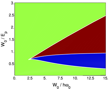
FIG. 1.: The “phase diagram” corresponding to the energy $E_{u}\left(\delta u\right)$, which represents the number of energy minima as a function of $W_{0}/\hbar\omega_{0}$ and $W_{0}/\left(\lambda^{2}/k\right)$. The green area corresponds to a singe minimum of $E_{u}$, while the blue and the red regions represent the parameters when the energy has two minima with the lowest being either the Holstein minimum (the blue region) or Migdal minimum (the red region).

Depending on the ratios of the electron bandwidth $W_{0}$ to the polaron energy $E_{p}\equiv\lambda^{2}/k$ and the phonon energy $\hbar\omega_{0}$, the function $E_{u}\left(\delta u\right)$ has either one or two minima. The corresponding phase diagram is presented in Fig. 1. In CMR compounds, the bandwidth $W_{0}\gg\hbar\omega_{0}$, and therefore the summation in Eq. (15) always includes two and only two terms. The minimum at small distortions, $\delta u^{(1)}\simeq\frac{\lambda^{2}\hbar\omega_{0}}{kc_{0}W_{0}\langle\cos\frac{\theta}{2}\rangle}$, which we will refer to as the “Migdal minimum”, corresponds to extended electron eigenstates with renormalized effective mass with the energy

$$E_{e}\simeq-x\left(1-x\right)\left[\frac{c_{0}}{2}W_{\theta}-\frac{\hbar\omega_{0}\lambda^{2}}{2kc_{0}W_{\theta}}\right]$$ (17)

The other minimum, which we will refer to as the ”Holstein minimum”, occurs at $u^{(2)}\simeq\lambda/M\omega_{0}^{2}$, and corresponds to small polarons with the energy

$$E_{p}\simeq-x\left(1-x\right)\left[\frac{c_{0}}{2}W_{\theta}\exp\left(-\frac{\lambda^{2}}{k\omega_{0}\hbar}\right)-\frac{\lambda^{2}}{2k}\right]$$ (18)

Substituting (17) and (18) into Eq. (15), we obtain:

$$F\left[P_{\vartheta}\right] = -T\log\left[\exp\left(-\frac{E_{e}}{T}\right)+\gamma\exp\left(-\frac{E_{p}}{T}\right)\right]$$ (19)

$$+ T\int d\vartheta\sin\vartheta P_{\vartheta}\left(\vartheta\right)\log P_{\vartheta}\left(\vartheta\right)$$ (20)

where $\gamma\simeq\sqrt{1+\frac{2c_{0}x\left(1-x\right)}{1+4x\left(1-x\right)}\frac{W_{\theta}}{\hbar\omega_{0}}}$

The equations (20), (17) and (18) define a variational problem for the spin distribution function $P_{\vartheta}$, which can be solved by a straightforward minimization of the free energy. The corresponding procedure is similar to the one used for the standard DE model and described in detail in Ref. [19]. We generally find a phase transition between low lattice distortion ferromagnetic phase at low temperatures and high lattice distortion paramagnetic phase at hight temperatures. For a strong electron-lattice coupling, $kW_{0}\lesssim\lambda^{2}$ , the transition is of the first kind, and is accompanied by the virtual collapse of the lattice distortion $\delta u$, as shown in Fig. 2. Note the remarkable similarity of the predicted behavior to the observations in recent experiments [10, 11], as illustrated by the inset.

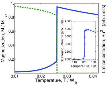
FIG. 2.: The magnetization $M/M_{\rm sat}$ (dashed blue line) and the lattice distortion $\Delta u$ in units of $\lambda/k$ (green line) as functions of temperature $T$ (in units of $W_{0}$), for the carrier concentration $x=0.3$. The inset shows the experimental temperature dependence of diffuse scattering intensity due to lattice distortion from Ref. [10].

In the other limit, when the electron-lattice coupling is small ( i.e. $kW\hbar\omega_{0}\gg\lambda^{2}$), our model corresponds to the standard double-exchange, and the transition is of the second kind. In fig. 3 (a) we plot the change of the lattice distortion $\delta u\equiv u_{2}-u_{1}$ at the phase transition, $\Delta u|_{c}$, as a function of the model parameters, $\lambda^{2}/kW_{0}$ and $W_{0}/\hbar\omega_{0}$, in false-color representation. There, the “deep blue sea” for small electron-lattice coupling corresponds to the second-order phase transition, where $\Delta u|_{c}\equiv 0$ by definition.

The phase transition changes from the first order kind to the second order when the ratio of the polaron energy $E_{p}\equiv\lambda^{2}/k$ to the electron bandwidth $W_{0}$ is near unity. This is in a remarkable agreement with experimental data, as these quantities in lanthanum manganites are believed to be of the same order, and both first[10, 11] and second-order phase transitions[20] are indeed observed in experiments depending on the composition (which is likely to affect the electron-lattice coupling and the bandwidth).

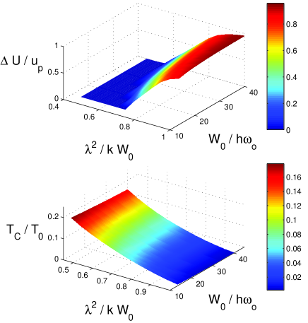
FIG. 3.: The change of lattice distortion at the transition in units of $u_{p}\equiv\lambda/k$ (top panel) and the critical temperature in units of $T_{0}\equiv\frac{c_{0}}{2}x(1-x)W_{0}$ (bottom panel), as functions of $\lambda^{2}/(kW_{0})$ and $W_{0}/\hbar\omega_{0}$, in false-color representation. The “deep blue sea” in the top panel represents the parameters for the second-order transition when $\Delta u\equiv 0$. The carrier concentration $x=0.3$.

An increase of the electron-lattice coupling leads to suppression of the metallic phase, which manifests itself in smaller values of the critical temperature. This behavior is illustrated in the bottom panel of Fig. 3 , where we present the false-color representation of the dependence $T_{c}$ as a function of both parameters of the model, $\lambda^{2}/kW_{0}$ and $W_{0}/\hbar\omega_{0}$.

An important feature of the proposed theory is the strong dependence of the critical temperature of the ferromagnetic transition on the effective ionic mass $M$. This behavior is illustrated in Fig. 4 where we plot the critical temperature (in units of the “bare” bandwidth $W_{0}$) vs. $\frac{k}{\hbar\omega_{0}}\lambda^{2}/k^{2}\sim\sqrt{M}$. As follows from Fig. 4, a 10% change in the oxygen ion mass which corresponds to the replacement of ${}^{16}O$ by ${}^{18}O$, could account for a variation of critical temperature by $~{}20\%$, which explains the recently observed giant isotope effect in lanthanum manganites.[12]

Note the remarkable “anti-correlation” of the change of the lattice distortion at the transition with the critical temperature, as seen from Fig. 3. This finding is again in agreement with the experimental data[20, 10, 11] : the transition of the second order kind is generally observed in the compounds with relatively high values of $T_{c}$, while a second-order transition is found in materials with a smaller value of critical temperature.

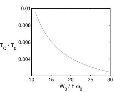
FIG. 4.: The critical temperature as a function of $W_{0}/\hbar\omega_{0}\sim\sqrt{M}$ (for a fixed value of $\lambda^{2}/(kW_{0})=1.$).

The dependence of $P_{u}(u_{1},u_{2})$ on $\Delta u$ in our ansatz for the distribution function (5) introduces the essential correlation of lattice distortion with electronic occupation. If this correlation is ignored by approximating $P_{u}(u_{1},u_{2})$ in a mean-field fashion by $p(u_{1})p(u_{2})$, the important results of our theory presented in Figs. 2-4 which include the collapse of the lattice disorder at first-order ferromagnetic transition and strong isotope effect in the critical temperature, cannot be obtained.

We conclude with a discussion of the effect of intrinsic disorder. The intrinsic disorder, which can be represented in the model Hamiltonian (1) by a term of the type $\sum_{i}V_{i}c_{i}^{\dagger}c_{i}$, favors less ordered paramagnetic phase and therefore leads to a decrease of the critical temperature. This effect was considered in detail in Ref. [19]. More important is the effect of the intrinsic disorder on the transport properties of the CMR compounds. In high quality samples with relatively weak disorder, the “Migdal minimum” describes the extended states and is responsible for the metallic behavior below the transition temperature.

If the electron-phonon coupling is substantial, the situation is dramatically different above the transition where the dominant contribution is given by the “Holstein minimum”. There, the effective bandwidth is exponentially suppressed due to lattice distortions

$$W_{H} \propto W_{0}\exp\left(-\frac{\lambda^{2}/k}{\hbar\omega_{0}}v^{2}\right)$$ (21)

where $\lambda^{2}/k\sim W_{0}\gg\hbar\omega_{0}$ (in manganites $W_{0}/\hbar\omega_{0}\sim 50$) and $v\equiv k\ \delta u/\lambda$ is the dimensionless lattice distortion which in the paramagnetic phase is of the order unity (see Fig. 2). Therefore $W_{H}\ll W_{0}$, and small intrinsic disorder in the CMR compounds will lead to the localization of the Holstein polarons. On the other side of the ferromagnetic transition, small intrinsic disorder alone, because of the vanishing spin as well as polaron disorder, is insufficient to localize the electronic states. So metallic conduction occurs below the ferromagnetic transition, while an activated form of resistivity is obtained above the transition, in agreement with experimental data.

In contrast, for low electron-phonon coupling constants, as evidenced for example by high (second-order) transition temperatures, in pure samples the resistivity is expected to be ”metallic” on both sides of the transition. Experimental results are consistent with these observations.

To summarize, in this paper a systematic method has been found to isolate and calculate the principal effects of electron-lattice interactions in strongly correlated materials of the double-exchange family. By including effects of the correlation of lattice vibrations with local electron occupation, we have shown that for the same reason that the itinerant state sweeps away spin-disorder, it also sweeps away lattice disorder. This has been accomplished by a variational form for the couple electron-lattice that extrapolates from the Holstein form to the Migdal form as the self-consistently determined bandwidth changes from a value small compared to polaron binding to a value large compared to it. The results of the calculations explain many of the peculiar features of the experimental results of CMR compounds.

We gratefully acknowledge the hospitality of the Aspen Center for Physics where a part of this work was done. E.N. would like to thank A. Tkachenko for helpful discussions.

- [1] S. Jink, T. H. Tiefel, M. McCormack, R. A. Ramesh, and L. H. Chen, Science 264, 413 (1994); M. I. Imada, A. Fujimori, and Y. Tokura, Rev. Mod. Phys. 70, 1039 (1998) and references therein.
- [2] A. P. Ramirez, J. Phys.: Condens. Matter 9, 8171 (1997).
- [3] N. Furukawa, J. Phys. Soc. Jpn 63, 3214 (1994).
- [4] N. Furukawa, preprint cond-mat/9812066 (1998).
- [5] L. Sheng, D. Y. Xing, D. N. Sheng, and C. S. Ting, Phys. Rev. Lett. 79, 1710 (1997).
- [6] L. Sheng, D. Y. Xing, D. N. Sheng, and C. S. Ting, Phys. Rev. B. 56, 7053R (1997).
- [7] C. Zener, Phys. Rev. 82, 403 (1951).
- [8] P. W. Anderson and H. Hasegawa, Phys. Rev. 100, 675 (1955).
- [9] P. G. de Genes, Phys. Rev. 118, 141 (1960).
- [10] S. Shimomura, N. Wakabayashi, H. Kuwahara, and Y. Tokura, Phys. Rev. Lett. 83, 4389 (1999).
- [11] L. Vasiliu-Doloc, S. Rosenkranz, R. Osborn, S. K. Sinha, J. W. Lynn, J. Mesot, O. H. Seeck, G. Preosti, A. J. Fedro, and J. F. Mitchell, Phys. Rev. Lett. 83, 4393 (1999).
- [12] G. M. Zhao, K. Conder, H. Keller, and K. A. Muller, Nature (London) 381, 676 (1996).
- [13] C. G. Kuper and G. .D. Whitfield, eds., Polarons and Excitons, Plenum Press, New York, 1968.
- [14] G. D. Martin, Many-Particle Physics, Plenum Press (1981).
- [15] U. Yu and B. I. Min, preprint cond-mat/9906263 (1999).
- [16] A. A. Abrikosov, L. P. Gorkov, and I. E. Dzyaloshinski, Methods of Quantum Field Theory in Statistical Physics, Dover, New York, 1977.
- [17] A. J. Millis, R. Mueller, B. I. Shraiman, Phys. Rev. B 54, 5389 (1996)
- [18] A. J. Millis, P. B. Littlewood, and B. I. Shraiman, Phys. Rev. Lett. 74, 5144 (1995).
- [19] E. E. Narimanov and C. M. Varma, to be published in Phys. Rev. B; C.M. Varma, Phys. Rev. B54, 7329 (1996).
- [20] Y. Tokura, A. Urushibara, Y.Moritomo, T.Arima, A.Asamnitsu, G. Kido, and N. Furukawa, J. Phys. Soc. Jpn 63, 3931 (1994).