Fractal analysis of Sampled Profiles: Systematic Study

Abstract

A quantitative evaluation of the influence of sampling on the numerical fractal analysis of experimental profiles is of critical importance. Although this aspect has been widely recognized, a systematic analysis of the sampling influence is still lacking. Here we present the results of a systematic analysis of synthetic self-affine profiles in order to clarify the consequences of the application of a poor sampling (up to 1000 points) typical of Scanning Probe Microscopy for the characterization of real interfaces and surfaces. We interprete our results in term of a deviation and a dispersion of the measured exponent with respect to the “true” one. Both the deviation and the dispersion have always been disregarded in the experimental literature, and this can be very misleading if results obtained from poorly sampled images are presented. We provide reasonable arguments to assess the universality of these effects and we propose an empirical method to take them into account. We show that it is possible to correct the deviation of the measured Hurst exponent from the “true”one and give a reasonable estimate of the dispersion error. The last estimate is particularly important in the experimental results since it is an intrinsic error that depends only on the number of sampling points and can easily overwhelm the statistical error. Finally, we test our empirical method calculating the Hurst exponent for the well-known 1+1 dimensional directed percolation profiles, with a 512-point sampling.

I Introduction

The characterization of interfaces and of the mechanisms underlying their formation and evolution is a subject of paramount importance for a broad variety of phenomena such as crystal growth, rock fracture, biological growth, vapor deposition, surface erosion by ion sputtering, cluster assembling, etc … (Barabasi and Stanley (1995); Mandelbrot (1982); Family and Landau (1984); Meakin (1998); Pietronero and Tosatti (1985) and references therein). Since the pioneering work of B.B. Mandelbrot, fractal geometry has been widely used as a model to describe these physical systems that are too disordered to be studied with other mathematical tools but that still hold a sort of “order” in a scale-invariance sense Barabasi and Stanley (1995); Mandelbrot (1982); Vicsek (1992). In particular, the growth of interfaces resulting from the irreversible addition of subunits from outside (vapor deposition of thin films, low energy cluster beam deposition, etc…) shows a typical asymmetric scale invariance, because of the existence of a privileged direction (e.g. the direction of growth) Kardar et al. (1986); Witten and Sander (1983); Family and Vicsek (1985); Messier and Yehoda (1985); Meakin et al. (1986); Meakin (1987, 1998); Lichter and Chen (1986); Family (1990); Krim and Palasantzas (1995); Csahok and Vicsek (1992); Bales et al. (1990); Muller-Pfeiffer et al. (1990); Sit et al. (1999); Yoona et al. (1999); Milani et al. (2001a, b); Buzio et al. (2000). These interfaces belong to the class of self-affine fractals and they can be described either by the fractal dimension $D$ or by the well-known Hurst exponent $H$ Peitgen,H.-O. and Saupe (1989); Meakin (1989); Voss (1989); Schmittbuhl et al. (1995a); Mandelbrot (1985, 1986). If these systems are the result of a temporally evolving process, they usually show also a time scale-invariance described by the exponent $\beta$ Vicsek (1992); Barabasi and Stanley (1995). Because of the close relationship between the scaling exponent(s) and the fundamental mechanisms leading to scale invariance, universality classes can be defined Vicsek (1992); Barabasi and Stanley (1995). An accurate knowledge of $H$ (and $\beta$) is required to identify the universality class of the system and to give a deep insight on the underlying formation processes.

The possibility of characterizing the topography of an interface in a dimension range from the nanometer up to several tens of microns, in a relatively simple and quick way by Atomic Force Microscopy (AFM) and Scanning Tunneling Microscopy (STM) Binnig et al. (1982, 1986) has stimulated an upsurge of experimental report claiming for self-affine structures (see Refs. Malcai et al. (1997); Avnir et al. (1998) and references therein). The abundance of experimental characterization of different systems and the limited sampling capability of the scanning probe microscopies (SPM) prompted at the attention of many authors the need of an accurate methodological approach to the determination of the exponent $H$ and of its error Deng et al. (1999a); Tate (1998), realistically considering the consequences of the finite sampling inherent to SPM. Typical sampling with an AFM or a STM is 256 or 512 points per line, for a maximum of 512 lines. Most of the results published in the late eighties and early nineties were based upon 256x256-point data-sheets, or even smaller ones (see list of references in Ref. Malcai et al. (1997)). Commercially available SPMs offer today a maximum of 512x512-point resolution, and homemade instruments hardly go beyond this value.

Many authors have questioned the reliability of the measurement of the Hurst exponent from a poorly sampled profile Dubuc et al. (1989); Schmittbuhl et al. (1995b); Mehrabi et al. (1997); Schmittbuhl et al. (1996). In order to quantify the influence of the sampling on the determination of $H$, a numerical analysis can be performed on artificial self-affine profiles, generated with a specific algorithm, with a fixed number of points $L$ and known Hurst exponent $H_{in}$. The “true” exponents ($H_{in}$) are then compared with the ones measured directly from the generated profiles ($H_{out}$). Usually a sensible discrepancy between the measured $H_{out}$ and the expected $H_{in}$ is found Dubuc et al. (1989); Mehrabi et al. (1997); Schmittbuhl et al. (1996). The discrepancy is not uniform but depends on the value of $H_{in}$. As one would expect, the discrepancy is globally dependent on the number $L$ and it approaches zero for large values of $L$. In particular, for $L<1000$ the sampling effect is of great importance since the discrepancy can be of the order of the exponent itself (100% relative error) Schmittbuhl et al. (1995b). Dubuc et al. have reported that even for values of $L$ as high as 16384, the discrepancy is still significant Dubuc et al. (1989).

Although the problem of sampling has been clearly addressed and discussed, quite surprisingly a systematic analysis of the problem, considering different generation algorithms, is still lacking. The dependence of the sampling effect on $L$ has been investigated Dubuc et al. (1989); Schmittbuhl et al. (1995b) and also many different methods for the measurement of $H_{out}$ have been considered for different values of $H_{in}$ in the range $[0.1-1]$ Dubuc et al. (1989); Schmittbuhl et al. (1995b); Mehrabi et al. (1997); Schmittbuhl et al. (1996). However, either only one single generation algorithm has been used Schmittbuhl et al. (1995b); Schmittbuhl et al. (1996), or the results from different generation algorithms have not been compared Mehrabi et al. (1997). We believe that this comparison is of fundamental importance.

Indeed profiles from different generation algorithms can be considered as different self-affine objects sampled in $L$ points. For a fixed value of $H_{in}$, these objects would all have the same fractal dimension if they were sampled with an infinite number of points. The fundamental question at this point is whether the discrepancy of $H_{out}$ from $H_{in}$, for a finite value of $L$, is the same for every self-affine object (i.e. for every generation algorithm). Only an analysis that considers different self-affine objects has a statistical validity and allows a reliable interpretation of the results. Up to now the results obtained in literature from a single generation algorithm did non allow a discussion of the nature of the aforementioned discrepancy, which has been interpreted as an uncontrollable error affecting the analysis of sampled profiles. The main conclusion drawn by these authors is the non-reliability of results obtained from profiles with less than 1024 sampling points Schmittbuhl et al. (1995b).

Our aim is to achieve a deeper understanding of the effects of sampling in order to answer the question whether the measurement of the Hurst exponent with a poor number of sampling points is reliable or not. This point is crucial both for future analysis of self-affine profiles and for a correct interpretation of the results already present in literature.

From a more general point of view, fractality is characterized by the repetition of somehow similar structures at all length scales and can be described in its major properties by a single number: the fractal dimension $D$ Falconer (1990); Mandelbrot (1982). Any finite sampling of a fractal object poses both an upper and a lower cut-off to this scale invariance. It has been shown that these cut-offs introduce a deviation in $D$ and the sampled object has a dimension different from the one of the underlying continuous object Dubuc et al. (1989); Schmittbuhl et al. (1996); Mehrabi et al. (1997). However, it is still unknown whether the sampling influences in a different way different objects characterized by the same ideal dimension, thus breaking the sort of universality that makes a fractal be identified by its dimension only.

In this paper we present a systematic analysis considering together all the generation algorithms found in literature. The aim of our analysis is to understand whether the discrepancy of the measured $H_{out}$ for a fixed $L$ and for every generation algorithm is completely random or has a universal dependence on $H_{in}$. The latter observation can be interpreted as a reminiscence of the fact that a fractal object is completely characterized by its dimension . The distinction is of crucial importance because in the case of universal dependence of $H_{out}$ on $H_{in}$ , one can empirically correct the discrepancy of the measured exponents from the “true” ones. Some authors independently suggested to use directly the $H_{out}$ vs. $H_{in}$ curves as correction, but they considered only one generation algorithm without discussing the universal character that these curves must have in order to be utilized for any self-affine object Deng et al. (1999a).

Conversely, on the basis of our analysis, we will interpret the discrepancy in terms of two distinct contributions: a universal deviation and a random dispersion. We will propose a powerful method to correct the universal deviation and we will discuss the nature of the dispersion, which is due to both statistical fluctuations and an intrinsic sampling effect. The latter turns out to be a sort of systematic error that cannot be corrected unless one knows the generation algorithm that produced the self-affine object. In the case of generic self-affine profiles which have not been generated by a specific algorithm, such as experimental profiles, the above arguments no longer hold. A new procedure to quantify the intrinsic error in the measurement of the Hurst exponent of generic self-affine profiles is thus needed.

On these basis, we will discuss the effect of sampling on the reliability of the fractal analysis of poorly sampled self-affine profiles, focusing on both the deviation and the dispersion of the measured exponents from the ideal ones, showing that the conclusions drawn by Schmittbuhl et al. that “… a system size less than 1024 can hardly be studied seriously, unless one has some independent way of assessing the self-affine character of the profiles and very large statistical sampling” were too restrictive Schmittbuhl et al. (1995b). Moreover, we will point out that the estimate of the intrinsic error is essential for a correct classification of a process in terms of universality classes. In fact, in order to distinguish exponents belonging to different classes, it is necessary to quantify the error on the measurement. Up to now, the statistical error or the error of the fit have been used to quantify the error on the measurement of $H$ Krim et al. (1993); Deng et al. (1999b); Iwasaki and Yoshinobu (1993). Both the statistical error and the error of the linear fit can be made very small, if a large number of profiles are averaged. However, if the measurement is likely to be affected by more subtle intrinsic errors, such as the aforementioned dispersion due to the sampling, considering only the statistical error may lead to serious misleading. The intrinsic error in many cases may indeed be much larger than the statistical one.

In the following sections we will present a systematic analysis of synthetic self-affine profiles with the aim of both achieving a deep understanding of the effects of sampling and providing the experimentalists of a reliable tool for the fractal analysis of surfaces and interfaces. To this purpose we have developed a new automated fitting protocol in order to avoid any arbitrariness in the measurement. With this new methodology we will study the effects of sampling, enlightening the main characteristics of the deviation and the dispersion of the measured exponents. We will present a new powerful method to correct the deviation of $H_{out}$ and to estimate the error of the measurement. Finally, we will apply our empirical correction procedure to 512-point profiles created with the directed percolation (DP) algorithm Buldyrev et al. (1992). This system provides a simple benchmark to test our protocol and allows noticing the opportunity of the correction.

II The Automated Fitting Protocol

Self-affine systems occurring in nature are usually profiles or surfaces. In order to measure their Hurst exponents the 2+1 dimensional case of surfaces is usually reduced to 1+1 dimensions, considering the intersection of the surface with a normal plane. The particular case of in-plane anisotropy results in a dependence of $H$ on the orientation of the plane with respect to the surface Dubuc et al. (1989); Schmittbuhl et al. (1995b); Falconer (1990); Barabasi and Stanley (1995).

Once we have scaled down the analysis to 1+1 dimensions, the following general properties characterize a self-affine profile. If $h(x)$ is the height of the profile in the position $x$, the orthogonal anisotropy can be expressed by the scaling relationship:

$$h(\lambda x)=\lambda^{H}h(x)$$ (1)

where $H\in(0,1)$ is the Hurst exponent, $\lambda$ is a positive scaling factor and the equation holds in a statistical sense Barabasi and Stanley (1995); Stanley (1971). The fractal dimension $D$ of the profile is related to the Hurst exponent by the equation $D=2-H$ while the dimension of the surface is $D=3-H$ Mandelbrot (1986); Moreira et al. (1994). The lower is $H$, the more space invasive is the surface. In most of the physical self-affine surfaces, the scale invariance does not extend to all length scales but there is an upper cut-off above which the surface is no longer correlated. The length at which this cut-off appears is defined as the correlation length $\xi$ Barabasi and Stanley (1995); Malcai et al. (1997). In the present analysis, we consider only profiles whose correlation length (expressed in number of points) is equal to their length $L$. To this purpose we have carefully studied each generation algorithm in order to grant the condition $\xi=L$. For this reason we were often forced to generate very long profiles and to consider only their central portion Makse et al. (1996); Mehrabi et al. (1997); Simonsen and Hansen (1999). The usual procedure to measure the Hurst exponent of a self-affine profile $h(x)$ is to calculate appropriate statistical functions from the whole profile. These functions of analysis (AFs) show a typical power law behavior on self-affine profiles:

$$AF[h(\cdot),k]=c\,k^{f(H)}$$ (2)

where $c$ is a constant, $k$ is a variable indicating the resolution at which the profile $h$ is analyzed (typically a frequency or a spatial/temporal separation), and $f(H)$ is a simple function of the Hurst exponent $H$ Mehrabi et al. (1997); Barabasi and Stanley (1995); Yang et al. (1997); Moreira et al. (1994); Peng et al. (1994); Press et al. (1986); Simonsen et al. (1998). The power law behavior of the AF is then fitted in a log-log plot in order to calculate the exponent $H$. In the analysis of statistical self-affine profiles there are random fluctuations super-imposed to this power law behavior. The signal-to-noise ratio of these fluctuations is scale-dependent, the AFs being calculated as averages of statistical quantities at different length scales Barabasi and Stanley (1995). To reduce this noise, the average of the AFs obtained from $N$ independent profiles is usually taken before the execution of the linear fit. However, while small-scale fluctuations are easily smoothed, larger scale fluctuations converge very slowly.

The identification of the linear region in the analysis of the AFs is a puzzling point. Windowing saturation is present at length scales comparable with the profile length depending on the nature of the profiles Yang et al. (1997). This results in a departure from the power law behavior to a constant value. Moreover, the degradation of the fractality due to the sampling causes a diversion of the AFs from their ideal power law behavior. This produces both a discrepancy of the measured Hurst exponent from the ideal value (a change of the slope in the log-log plot) and a shortening of the linear region as shown in Fig. 1.

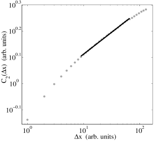
Figure 1: Average height-height correlation function $C_{2}$ calculated from $N=500$ profiles of $L=512$ points, generated with the random addition method with Hurst exponent $H_{in}=0.1$. It is also shown the linear region and the fit obtained with the automated fitting protocol (AFP). One can clearly see the overall curved shape due to the sampling.

Here, the presence of curved regions is clearly visible. It can be seen that this anomalous behavior is not localized at length scales close to the length of the profile, but involves also the shortest length scales especially for values of $H$ close to zero. It is important to notice that this effect is not due to experimental conditions, such as the finite size of the SPM scanning probe. Thus it is necessary, in particular for small values of $H$, to chose a linear region instead of fitting the whole function. The methods proposed in the literature to identify the linear region (e.g. the consecutive slopes method Bourbonnais et al. (1991); Barabasi and Stanley (1995), correlation index method Barlow (1989), the coefficient of determination method Hamburger et al. (1996) and the “fractal measure” method Li et al. (1999)) are usually based on an arbitrary (human) choice. This is particularly delicate since the curvature in the AFs can be so small, if compared to the statistical noise, that it is hard to distinguish the correct linear region. Because of this reason, we think that the proposed methods suffer of a high degree of arbitrariness. Moreover, all these methods make no distinction between a straight line with statistical noise and a slightly curved line.

Due to the previous arguments and since no universally accepted fitting procedure is available in literature, we were prompted to develop an automated fitting protocol (AFP) with two purposes: to reduce as much as possible the effects of the curved regions on the measured exponent, and to define a standard algorithm for the choice of the linear region, eliminating, as much as possible, any arbitrariness. This is very important for the reliability of the results, in particular for the comparison of different generation algorithms. Moreover, the automation of the fitting procedure is essential to perform a systematic analysis. In fact, in order to have good statistics, a large number of AFs must be calculated and fitted.

In our procedure, that is an implementation of the consecutive slopes algorithm Barabasi and Stanley (1995), the curve to be fitted is divided in many portions of the same length $\ell$ (in number of points) and each of them is considered separately. A linear and a cubic fit are performed on each portion. Comparing the mean distance of the linear fit from the portion to the mean distance of the cubic from the linear fit, we evaluate whether the portion is almost linear with uncorrelated noise or it presents a definite curvature. Obviously, the distinction is not immediate and we have to set a threshold to separate the two cases through a parameter in the fitting procedure. The use of a parameter is common to other methods (see for example the coefficient of determination method used in Ref. Hamburger et al. (1996)). Once the fitting parameter is set, our procedure is able to decide automatically whether the portion is “curved” or “linear”. Only the “linear” portions are then considered. They undergo a straight-line-fit analysis through which the slopes and their errors are determined. A distribution of the slopes weighted with the values of the errors is then built (see Fig. 2a) and its main peak position and width are measured. We do not consider here the presence of more than one linear region with different slopes. Thus, there is a well-defined main peak in the distribution. We have extended our procedure also to the case of more than one linear region, but this extension is out of the scopes of this article.

The procedure described above is repeated varying the length $\ell$ of the portions from a minimum value $\ell_{min}$ up to the length of the curve. The results are then shown in a plot of the peak position (i.e. a slope value) versus the length of the portion, with the peak widths as error bars (see Fig. 2b).

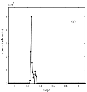
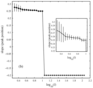
Figure 2: Application of the fitting protocol step by step: (a) the distribution of the slopes for a single value of the length $\ell$ of the portion ($\ell=0.35$ decades) and (b) the final plot of the slopes (peak positions) vs. $\ell$, with an inset magnification showing the error bars.

If the analyzed curve presents a linear region, this plot shows a plateau for $\ell$ ranging from $\ell_{min}$ to the length of the whole linear region. This plateau is usually very easy to be identified because of the distinction between linear and curved portions. In fact, portions of length larger than the length of the whole linear region are considered curved portions and discarded. Thus, the plot usually drops to zero at the end of the plateau. Eventually, through an average and a standard deviation, we obtain the final slope value and its fitting error, while the length of the plateau gives the length of the linear region. In conclusion, our AFP is able to identify not only the slope of the linear region but also its length. We have tested our AFP before its application to the systematic analysis and we have found that the measured Hurst exponent is widely independent of the fitting parameter . Conversely, the length of the linear region strongly depends upon the value of the parameter and must be considered only an internal parameter of the analysis and not a direct measurement of the scale invariance range.

III Numerical Analysis

With all the generation algorithms published in literature we have created sampled self-affine profiles with known fractal dimension $D=2-H$. We have varied the exponent $H$ between 0.1 and 1 and we have focused on the value $L=512$ sampling points (the best sampling obtainable with most of the SPMs). We discuss also different values of $L$ up to 16384. Because there exists only a few algorithms that generate exactly self-affine profiles, we have used algorithms that generate statistically self-affine profiles, which are more difficult to handle but closer to reproduce natural physical systems. The algorithms we have used are known in literature as: the random midpoint displacement Schmittbuhl et al. (1995b); Voss (1986a), the random addition algorithm Feder (1988); Peitgen,H.-O. and Saupe (1989), the fractional Brownian motion Feder (1988), the Weierstrass-Mandelbrot function Lopez et al. (1994); Berry and Lewis (1980), the inverse Fourier transform method Voss (1986a) and a variation of the independent cut method Falconer (1990). For the measurement of the Hurst exponent of self-affine profiles we have used the height-height correlation function $C_{2}$ Yang et al. (1997) and the root mean square variable bandwidth with fit subtraction method Moreira et al. (1994); Peng et al. (1994). The value of $H_{out}$ has been calculated from the slope in the log-log plot of the average over $N$ statistically independent AFs, measured with our AFP.

The results are expressed in terms of $H_{out}$ vs. $H_{in}$ plots. Each plot is characteristic of a single AF and generation algorithm and it represents the relationship between the measured Hurst exponent $H_{out}$, calculated from the average of $N$ AFs, and the nominal exponent $H_{in}$ of the profile. Grouping the $H_{out}$ vs. $H_{in}$ plots obtained using the same AF for all the generation algorithms, the dispersion of the $H_{out}$ values comes to evidence.

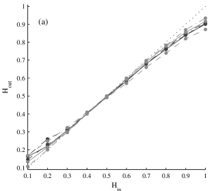
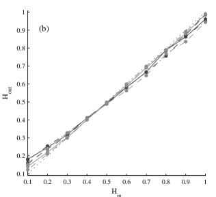
Figure 3: $H_{out}$ vs. $H_{in}$ graphs calculated from N = 500 profiles of L = 512 points each: (a) Height-height correlation function and (b) Root mean square variable bandwidth (with fit subtraction). The black dotted line represents the ideal $H_{out}=H_{in}$ behavior. The other line styles are related to different generation algorithms: random midpoint displacement (black continuous line), inverse Fourier transform (black dashed line), random addition (black dash-dotted line), Weierstrass-Mandelbrot (grey continuous line), fractional Brownian motion (grey dashed line) and independent cut (grey dash-dotted line).

In Fig. 3 we show the $H_{out}$ vs. $H_{in}$ graphs obtained from $N=500$, $L=512$ profiles, as explained in the previous section. We show separately in Figs. 3(a) and 3(b) the different AFs used. Since the profiles are statistically self-affine, the measured $H_{out}$ are subject to a statistical error that is inversely related to $N$ Deng et al. (1999b). In order to characterize the dependence of this statistical error on the number $N$ of averaged AFs, we let $N$ vary from 1 to 50 using the same profiles considered in Fig. 3. With these values of $N$ we have repeated the numerical analysis (i.e. calculation of the AFs, averaging and application of the AFP) and we have extracted a standard deviation $\sigma_{N}$ of the measured exponents.

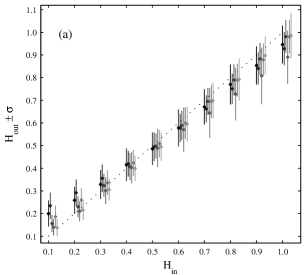
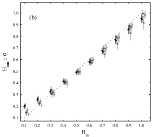
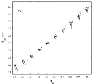
Figure 4: $H_{out}$ vs. $H_{in}$ graphs with error bars equal to twice the standard deviation $\sigma_{N}$ of the measured exponents. These graphs correspond to different values of the number $N$ of statistically independent profiles from which an average Hurst exponent is measured: (a) $N=1$, (b) $N=10$ and (c) $N=50$. It can be seen that for $N>10$ and for $H_{in}<0.3$ the overlap between the error bars corresponding to different generation algorithms is small or completely absent. For the sake of clarity we do not distinguish between different generation algorithms

.

In Fig. 4 we show the $H_{out}$ vs. $H_{in}$ graphs, analogous to those in Fig. 3, with the calculated error bars (twice the standard deviation $\sigma_{N}$), for a few values of $N$. We present the results for a single AF (the root mean square variable bandwidth with fit subtraction), the results for the other AFs being similar.

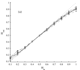
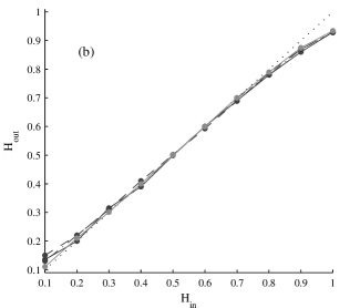
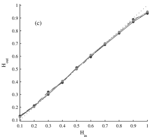
Figure 5: $H_{out}$ vs. $H_{in}$ graphs calculated with the height-height correlation function from: (a) $N=500$, $L=512$ profiles. (b) $N=50$, $L=4096$ profiles. (c) $N=15$, $L=16384$ profiles. Line styles are the same as in Fig. 3.

In Fig. 5 we show three $H_{out}$ vs. $H_{in}$ graphs obtained respectively with $N=500$, $L=512$ profiles, $N=50$, $L=4096$ profiles and $N=15$, $L=16384$ profiles. Again, we present only one AF (the height-height correlation function $C_{2}$).

IV Results and Discussion: Deviation and Dispersion from the Ideal Behavior

Ideal continuous fractal profiles are statistically characterized by their fractal dimension (universality) and their $H_{out}$ vs. $H_{in}$ graphs are straight lines Barabasi and Stanley (1995); Feder (1988); Falconer (1990).

In Fig. 3 a deviation from the ideal behavior is observed for both the AFs. It turns out that the sampling of a profile affects in a different way different methods of analysis. The deviation from the ideal behavior has been already observed in literature (for example, see Ref. Schmittbuhl et al. (1995b)) and our results are in good agreement with the previous ones.

Moreover, within the same method of analysis we observe that the different generation algorithms give significantly different $H_{out}$ vs. $H_{in}$ plots. This dispersion is pointed out here for the first time because different generation algorithms are considered together. The significance of the dispersion can be inferred from the characterization of the statistical error of the measured exponent discussed hereafter.

In Fig. 4 we show that for $N>25$ and $H_{out}<0.3$ the error bars of $H_{out}$ for different generation algorithms hardly overlap. This fact suggests that the statistical error is not the only reason of the differences between the $H_{out}$ vs. $H_{in}$ plots shown in Fig. 3.

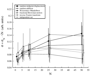
Figure 6: Graph of the statistical standard deviation $\sigma$ of the Hurst exponent, obtained from the definition of the standard deviation of the mean (Eq. (3)), vs. the number $N$ of averaged AFs. It can be clearly seen the saturation for values of $N$ bigger than 25 for almost all the generation algorithms.

In Fig. 6 we plot the statistical error $\sigma_{N}$ times the square root of $N$ vs. $N$. For $N\geq 10$ the curves approach a constant value according to the relationship between the standard deviation of independent, normally distributed measurements and the standard deviation of the mean upon $N$ measurements:

$$\sigma_{N}=\frac{\sigma}{\sqrt{N}}$$ (3)

This result shows that the AFP and the averaging of the AFs do commute. The assessment of this property is non-trivial due to the complexity of the AFP. Thus, we extrapolate the statistical error of the measured exponents in Fig. 3 ($N=500$) using Eq. (3) where $\sigma$ is extracted from the plateau in Fig. 6. Overestimating $\sigma$ with the value 0.16 we obtain $\sigma_{500}=0.007$. This value produces an error bar in Fig. 3 as small as the symbol used to mark the data. A direct calculation of $\sigma_{500}$, obtained averaging AFs calculated on groups of $N=500$ profiles for every $H\in[0.1,1]$ and for every generation algorithm, fitting and extracting a mean value and a standard deviation of $H$, would have required a huge and time consuming calculation.

These results suggest that the observed dispersion between the $H_{out}$ vs. $H_{in}$ curves for different generation algorithms is an intrinsic effect of the sampling, depending only on the number of sampling points $L$. This fact has an important consequence on a fractal analysis of experimental surfaces. While looking at a real sample, we do not know what kind of “algorithm” has generated the surface. This introduces an uncertainty on its real fractal dimension independent of the statistical error. Thus, there is an intrinsic upper limit to the precision of the measurement of the exponent. It is useless to strengthen the statistics once the number of acquired profiles makes the statistical error smaller than the intrinsic dispersion.

In Fig. 5 we see that as $L$ increases both the deviation and the dispersion decrease in agreement with their expected vanishing in the limit of $L$ going to infinity Schmittbuhl et al. (1995b). This is also an a posteriori proof of the correctness of both the generation algorithms and the methods of analysis.

Our interpretation of these effects is that the sampling of a self-affine profile lessens its fractality in such a way that it is no longer characterized universally by its fractal dimension (or Hurst exponent). While for a continuous self-affine profile the relationship $H_{out}=H_{in}$ holds, for sampled profiles we can see that different AFs produce different $H_{out}$ vs. $H_{in}$ plots from the same sampled fractal profile. Considering instead a single AF, our results show that sampled fractal profiles generated with different generation algorithms but with the same ideal dimension give different measured Hurst exponents.

However, Fig. 5 clearly shows that the lessening of fractality of a profile is rather a continuous process than a sharp transition: the poorer is the sampling, the worse are the deviation and the dispersion. In Figs. 5 and 3 we observe that the lessening of fractality acts in a similar way on profiles generated with different algorithms. The common trend of the $H_{out}$ vs. $H_{in}$ curves obtained from different generation algorithms is interpreted as a consequence of the universality of fractal objects.

It is then reasonable to assume the existence for every AF of a universal region in the $H_{out}$-$H_{in}$ plane containing all the $H_{out}$ vs. $H_{in}$ plots obtained with every possible generation algorithm. This region, approximately identifiable with the envelope of the $H_{out}$ vs. $H_{in}$ plots, has a width that depends on the number of sampling points and approaches the 1-dimensional $H_{out}=H_{in}$ ideal curve for very large values of $L$. We expect that, given any continuous self-affine profile with a Hurst exponent $H_{in}$ and given the exponent $H_{out}$ measured from an $L$-point sampling of the continuous profile, the pair ($H_{in}$,$H_{out}$) belongs to the universal region of the corresponding graph (specific for every AF and number of sampling points $L$). Provided a good characterization of the aforementioned regions (i.e. using as many generation algorithms as possible), we can use them to generate calibration graphs for every $L$ and AF describing the relationship between the measured $H_{out}$ and the true value $H_{in}$.

To produce the calibration graphs we proceed as follows. First of all, we make two general assumptions in order to take quantitatively into account the problem of measuring the Hurst exponent of a sampled profile. We assume that the $H_{out}$ values corresponding to the same $H_{in}$ are normally distributed around a mean $\langle H_{out}\rangle$, and we assume also that the values obtained with the available generation algorithms are a random sampling of the gaussian distribution. We then measure the average and the standard deviation of the dispersed $H_{out}$ values corresponding to each $H_{in}$ separately. Thus we obtain a sampling of the functions describing the dependence of $\langle H_{out}\rangle$ and $\sigma_{H_{out}}$ from $H_{in}$. With an interpolation algorithm using smooth functions, we derive the curve representing the relationship between $\langle H_{out}\rangle$ and $H_{in}$. We also derive the pair of curves corresponding to $\langle H_{out}\rangle+n\sigma_{H_{out}}$ and $\langle H_{out}\rangle-n\sigma_{H_{out}}$ vs. $H_{out}$ which define the $n$-th confidence level. For every value of $H_{out}$ it is possible to find the confidence interval of $H_{in}$ for any given confidence level. The resulting graphs for $L=512$ are shown in Fig. 7.

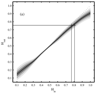
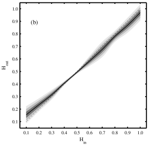
Figure 7: Calibration graphs $H_{out}$ vs. $H_{in}$ for the methods of analysis used in this article: (a) height-height correlation function and (b) variable bandwidth with fit subtraction. From the value of the measured exponent, one can easily extract the corresponding confidence interval of the corrected exponent, as represented graphically in (a).

These calibration graphs allow to take into account the deviation and the dispersion due to the sampling. A similar method has been independently proposed in Ref. Deng et al. (1999a) even though the analysis was limited to a single generation algorithm and the discussion on the reliability of the calibration regions together with the intrinsic dispersion were completely neglected.

Using the calibration graphs it is possible to measure the Hurst exponent of poorly sampled profiles correcting for the first time the deviation due to the sampling and providing a reasonable estimate of the error on a confidence level basis. The quantification of the error is of paramount importance, as pointed out in the introduction, since many authors estimated the error from the precision of the linear fit Krim et al. (1993); Iwasaki and Yoshinobu (1993) or from the standard deviation of the measured exponents Deng et al. (1999b). Our results show that they usually underestimated the true error.

V Application of the calibration graphs to the study of directed percolation numerical profiles

We have applied our procedure to the 1+1 dimensional directed percolation (DP) model, described by S.V. Buldyrev et al. Buldyrev et al. (1992). This model mimics the paper wetting process by a fluid. The resulting pinned interface is self-affine with exponent $H\simeq 0.63$.

We have analyzed $N=30$, $L=16384$ DP profiles with the height-height correlation function (h.-h. corr) and the variable bandwidth with fit subtraction (vbw), using the automated fitting protocol to measure the Hurst exponents. The results are shown in the second column of Tab. 1. We have not calculated the statistical error (see Section IV) because it would have been excessively time consuming. Thus, the error shown is simply the error of the fit calculated with the AFP.

Table 1: Measured Hurst exponents of sampled DP profiles (theoretical value: $H\simeq 0.63$ Buldyrev et al. (1992))

	$H_{out}^{16384}$	$H_{out}^{512}$	$H_{in}^{512}\;(68\%)$
h.-h. corr.	$0.615\pm 0.004$	$0.609\pm 0.002$	$[0.613-0.635]$
vbw	$0.620\pm 0.003$	$0.608\pm 0.012$	$[0.611-0.644]$

The values of the measured exponents $H_{out}^{16384}$ are significantly lower than the ones predicted by the DP model, suggesting that a correction is needed even in the case of profiles of $L=16384$ points, which are widely considered as continuous.

We have then analyzed $N=1000$, $L=512$ profiles extracted from the $L=16384$ profiles. We have applied the correction procedure based on the calibration graphs shown in Fig. 7 to the exponents measured with the AFP. In the third column of Tab. 1, the uncorrected measured exponents ($H_{out}^{512}$) are shown. The error is calculated as the root mean square (rms) value of the statistical error $\sigma_{1000}$ (evaluated as explained in Section IV) and the error of the fit calculated with the AFP. In the fourth column, the confidence intervals corresponding to the $68\%$ probability for the “true” exponents are shown ($H_{in}^{512}\;(68\%)$).

The results summarized in Tab. 1 allow to notice the effectiveness of the calibration graphs in the analysis of self-affine profiles when the effects of sampling are non negligible. In the example reported here, the poor sampling causes a discrepancy of about $4\%$ between the measured exponents and the theoretical one for DP profiles. After the correction with the calibration graphs, the expected value $H_{in}\simeq 0.63$ is consistent with the confidence intervals of the three AFs. Moreover, the intrinsic error due to the dispersion (about half the width of the confidence interval) turns out to be usually one order of magnitude larger than the aforementioned rms error.

In conclusion, our calibration graphs have allowed to correct the deviation and to quantify the intrinsic error of the Hurst exponent of poorly sampled ($L=512$) DP profiles.

VI Conclusions

We have carried out a systematic analysis in order to achieve a deeper understanding of the effects of sampling on the measurement of the Hurst exponent of self-affine profiles. This is a crucial point for the assessment of the reliability of fractal analysis of experimental profiles, such as topographic profiles of growing thin films and interfaces acquired with a Scanning Probe Microscope. We have pointed out that some of the steps leading to the measurement of the Hurst exponent have been only superficially discussed, although worth of deeper attention. We have focused on the quantification of the effects of sampling and possibly on their correction, allowing a more reliable identification of the universality class of growth.

In order to perform such a quantitative analysis we have developed a new automated fitting protocol that allows to remove the ambiguity in the choice of the region for the linear fit of the analysis functions. This point is usually underestimated in the published experimental literature, and appears to be a significant source of error in the whole analysis. Moreover, an automated protocol sensibly reduces the time required for the fitting of a large number of noisy curves, allowing a higher statistics. With our automated fitting protocol we have systematically investigated synthetic self-affine profiles generated with all the generation algorithms found in literature using different method of analysis.

The systematic analysis presented in this paper has been carried out on 1+1 dimensional profiles and we have not considered 2-dimensional methods of analysis (e.g. see Deng et al. (1999a); Krim et al. (1993)). However, it is reasonable to suppose that even in this case the effects of sampling cannot be neglected, and the conclusions drawn in Ref. Deng et al. (1999a) are probably incorrect. The similarity between Fig. 1 in Ref. Deng et al. (1999a) and the analogous results presented in this paper (see the variable bandwidth analysis of profiles generated with the random midpoint displacement shown in Fig. 3c) suggests that conclusions very close to those presented here can be drawn also in the 2-dimensional case.

Studying the discrepancy between the measured Hurst exponent $H_{out}$ and the “true” one ($H_{in}$) for synthetic self-affine profiles with $L=512$ points, we have shown that the main effects of sampling are a deviation of the $H_{out}$ vs. $H_{in}$ plots from the ideal behavior and a dispersion of the exponents calculated from different generation algorithms. Both these effects smoothly reduce with increasing values of $L$. The deviation turns out to be universal in the sense that the trend of the $H_{out}$ vs. $H_{in}$ curves is common to all of the generation algorithms, depending only on the number of sampling points and on the function used in the analysis. We propose that this behavior is reminiscent of the fact that a fractal object is completely characterized by its dimension and therefore the deviation can be at least empirically corrected. The dispersion instead has to be considered as an intrinsic error due to the sampling, but for the very special case of profiles whose generation algorithm allows to build their specific $H_{out}$ vs. $H_{in}$ plot. This dispersion error must be quantitatively taken into account since it cannot be reduced with an increase in the statistics but only with an increase in the number of sampling points.

The existence of an intrinsic dispersion error in the measurement of the Hurst exponent that depends only on the number of sampling points is very important. In fact, this intrinsic error easily overwhelms the statistical error for poorly sampled profiles. It is definitely clear that a reliable result cannot be based on the consideration of the statistical error only. Moreover, the dispersion poses an upper limit to the precision in the measurement of the Hurst exponent of sampled profiles. It becomes useless to increase the statistics once the statistical error has been made reasonably smaller than the intrinsic one. This is particularly important in an experimental analysis because it usually reduces significantly the number of profiles that have to be acquired, making the analysis much less time consuming.

Thanks to our systematic analysis, we have built, for each method of analysis, a calibration graph representing the region of the $H_{out}$-$H_{in}$ plane where the true exponents fall within a given confidence level. We have originally proposed to use these graphs as a reliable empirical method to correct the measured value of the Hurst exponent of a poorly sampled profile and to estimate its intrinsic sampling error. The reliability of the calibration graphs is based on two assumptions:

1. The measured exponents for all the possible self-affine profiles, with the same “true” exponent $H_{in}$ and with the same number of sampling points, are normally distributed;

2. The numerical generation algorithms known in literature provide a statistically reliable sample of all the possible self-affine profiles.

Even though we have found just six generation algorithms in literature, we believe that they still allow to obtain reasonable results or at least the only ones obtainable to date. These results represent a step forward to a reliable fractal analysis of both numerical and experimental profiles and to the individuation of the universality classes in the study of the evolution of many different systems.

In conclusion, we have demonstrated that a reliable measurement of the Hurst exponent of poorly sampled self-affine profiles is possible, provided that the measured $H_{out}$ is corrected of its deviation and that the sampling error is quantitatively taken into account. We have thus given strength to experimental analyses, since the numerical results reported in literature to date led to the conclusion that the analysis of self-affine profiles sampled with less than 1000 points is not reliable Schmittbuhl et al. (1995b). Even with the great improvement introduced by the use of the calibration graphs in the analysis of self-affine profiles, we definitely agree with Schmittbuhl et al. in pointing out that the comparison of the results obtained with different method of analysis is of fundamental importance Schmittbuhl et al. (1995b). Furthermore, we shortly comment on the common experimental procedure of connecting AFs calculated from profiles acquired with different scan sizes Krim et al. (1993); Iwasaki and Yoshinobu (1993); Fang et al. (1997). This connection allows investigating a wider range of length scales with a limited number of sampling points and makes the measurement more reliable. However, the deviation and dispersion are not influenced by this procedure, since they depend only on the number of sampling points of the profiles on which the AFs are calculated.

The AFP and the calibration graphs have been tested on numerically generated 1+1 dimensional directed percolation (DP) profiles, which have provided a benchmark to check our protocol. We have shown that for $L=512$ profiles a correction is needed and the calibration graphs allow to recover the theoretical value of $H$ predicted by the DP model. We have also shown that a correction is needed even for the $L=16384$ profiles, which are widely considered as continuous.

Our results provide a powerful tool for the accurate extraction of the Hurst exponent from poorly sampled profiles, and for the quantification of the error in the measurement. This is of paramount importance for experimentalists who study the scale invariance of surfaces and interfaces by Scanning Probe Microscopy or other techniques, with the aim of identifying the underlying universality classes. The huge amount of experimental results published in the past two decades about the fractality of many interfaces can be now analyzed under a new light.