From ballistic motion to localization: a phase space analysis

Abstract

We introduce phase space concepts to describe quantum states in a disordered system. The merits of an inverse participation ratio defined on the basis of the Husimi function are demonstrated by a numerical study of the Anderson model in one, two, and three dimensions. Contrary to the inverse participation ratios in real and momentum space, the corresponding phase space quantity allows for a distinction between the ballistic, diffusive, and localized regimes on a unique footing and provides valuable insight into the structure of the eigenstates.

The behavior of a quantum particle in a disorder potential depends significantly on the disorder strength. If the mean free path exceeds the system size, one may think of plane waves characterized by a fixed momentum which are scattered by the weak random potential. On the other hand, sufficiently strong disorder leads to exponentially localized states in real space. Then a wide range of momenta is needed to construct these states. A description for arbitrary disorder strength thus requires to adequately take into account real space as well as momentum space properties. In this paper, we will therefore adopt a phase space approach.

Signatures of the different regimes can already be found in the energy spectrum. While for weak and strong disorder energy levels can almost be degenerate, level repulsion occurs in an intermediate regime. Making use of random matrix theory the chaotic nature can be verified and related to diffusive motion. However, such considerations cover only statistical properties of the spectrum and do not give information about the structure of individual states.

A popular way to investigate the properties of single states is the calculation of their inverse participation ratio. In real space this quantity has frequently been employed mirli00 to measure the size of the localization domain of quantum states in the localized regime and to characterize the Anderson transition abrah79 ; lee85 . However, the real space inverse participation ratio is not very sensitive to changes in extended wave functions when going from the ballistic to the diffusive regime. In order to obtain a meaningful description of the structure of quantum states for all regimes on a unique footing, we generalize the concept of the inverse participation ratio to phase space.

The Anderson model of disordered solids ander58 has been the subject of extensive investigations over the last decades krame93 . A numerical study of this model in one, two, and three dimensions will demonstrate the virtues of our approach. In particular, we will be able to identify ballistic, diffusive, and localized regimes via properties of the eigenstates. In one dimension the results will significantly differ from those in higher dimensions, which can be attributed to the absence of a diffusive regime.

We start by introducing the relevant phase space concepts. At this point there is no need to specify the details of the disordered system except that we will consider a $d$-dimensional lattice model with lattice constant $a$ and length $L$ in each direction. In order to keep the notation simple, we will give the formulae for the case of one dimension, which can be generalized to higher dimensions in a straightforward manner.

A positive definite density in phase space is given by the Husimi function husim40 or Q function cahil69

$$\varrho(x_{0},k_{0})=|\langle x_{0},k_{0}|\psi\rangle|^{2}\,.$$ (1)

Here, the state $|\psi\rangle$ is projected onto a minimal uncertainty state $|x_{0},k_{0}\rangle$ centered around position $x_{0}$ and momentum $k_{0}$. In position representation, the latter assumes a Gaussian form

$$\langle x|x_{0},k_{0}\rangle=\left(\frac{1}{2\pi\sigma^{2}}\right)^{1/4}\exp\left(-\frac{(x-x_{0})^{2}}{4\sigma^{2}}+ik_{0}x\right)$$ (2)

where the value of the variance $\sigma^{2}$ is yet undetermined. The Husimi function is normalized, $\int(dxdk/2\pi)\varrho(x,k)=1$, and, for real wave functions $\psi(x)$, obeys the symmetry $\varrho(x_{0},k_{0})=\varrho(x_{0},-k_{0})$.

Figure 1: The Husimi function of a state at the band center is shown for a one-dimensional Anderson model of size $L=128$ with disorder strengths $W=0.1,1,2.5,10$, and $25$ increasing from left to right. Exploiting the symmetry with respect to $k=0$ the Husimi function is plotted on a linear and logarithmic scale in the upper and lower half, respectively. The gray values from white to black for increasing Husimi function have been normalized separately in each panel. The width $\sigma$ of the Gaussian (2) is indicated by the black square in panel (e).

The variance $\sigma^{2}$ of the Gaussian (2) determines the relative importance of real and momentum space. In the following, we choose $\sigma^{2}=La/4\pi$ leading to equal widths of the Gaussian in $x$- and $k$-direction. In order to obtain sufficient resolution, one has to ensure that $\sigma\ll L$ which limits the possible system sizes from below. Then, the effect of neglecting the tails of the Gaussian in finite size systems in presence of periodic boundary condition will also be small. Examples of Husimi functions for one-dimensional disordered systems are presented in Fig. 1, which will be discussed in detail below.

In higher dimensions, Husimi functions can no longer be visualized easily. A more global description of the phase space properties of the state is therefore necessary and often sufficient. Based on the Husimi function the so-called Wehrl entropy wehrl79 ; mirba95 ; gnutz01 is defined, which represents a measure of the phase space occupation. It was shown for the driven rotor that the Wehrl entropy of individual quantum states is connected to the energy level statistics gorin97 . A very similar system, the kicked rotor, can be mapped onto the Anderson model fishm82 , suggesting that the Wehrl entropy is a useful quantity for the characterization of the eigenstates of the Anderson model weinm99 .

For practical purposes it is more convenient to introduce the inverse participation ratio in phase space

$$P=\int\frac{dx\,dk}{2\pi}\,[\varrho(\vec{x},\vec{k})]^{2}\,,$$ (3)

which corresponds to a linearization of the Wehrl entropy varga94 . This inverse participation ratio can be compared directly to the corresponding quantities $P_{x}=\int dx|\psi(x)|^{4}$ and $P_{k}=\int dk|\tilde{\psi}(k)|^{4}$ in real and momentum space, respectively. $P_{x}$ is particularly well studied as it is related to the probability for a diffusing particle to return to its original position in the long-time limit thoul74 .

Furthermore, $P$ can be evaluated without recourse to the $2d$-dimensional Husimi function. In fact, only the wave function $\psi(x)$ is required since we can recast (3) in the form

$$P=\frac{1}{8\sqrt{\pi}\sigma}\int du\,\left|\int dv\,\psi\!\left(\frac{1}{2}(u-v)\right)\psi\!\left(\frac{1}{2}(u+v)\right)\right.$$ (4)

$$\times\left.\exp\left(-\frac{v^{2}}{8\sigma^{2}}\right)\right|^{2}\,.$$

Its nondiagonal character provides the information on momentum. It is only by means of (4) that one succeeds in determining the inverse participation ratio for three-dimensional systems.

In the following, we specifically consider the Anderson model for non-interacting electrons on a lattice with periodic boundary conditions, where disorder is modeled by a random on-site potential. In $d=1$, the Hamiltonian reads

$$H=-t\sum_{n}(|n\rangle\langle n+1|+|n+1\rangle\langle n|)+W\sum_{n}v_{n}|n\rangle\langle n|$$ (5)

with Wannier states $|n\rangle$ localized at sites $n=1,\dots,L$. All lengths are measured in units of the lattice constant $a=1$. The hopping matrix element $t=1$ between neighboring sites defines the energy scale. The on-site energies $v_{n}$ are drawn independently from a box distribution on the interval $[-1/2;1/2]$ and $W$ denotes the disorder strength.

Husimi functions for a state at the band center are presented in Fig. 1 for increasing disorder strength $W$ and a randomly selected disorder realization $v_{n}$. Making use of the symmetry with respect to $k=0$, the Husimi function is plotted on a linear and logarithmic gray scale in the upper and lower half, respectively. White points in the lower half may be related to the zeros of the Husimi function leboe90 .

For $W=0.1$ (Fig. 1a), the disorder represents only a small perturbation and the Husimi function is thus still close to that of plane waves. Except for the states at the band edges, one finds two stripes well localized at the corresponding $k$-values, which are extended over the full real space. The width of the stripes is induced by the projection onto the Gaussian (2). In Fig. 1e the opposite limit is depicted. At $W=25$, the hopping is a small perturbation, $t\ll W$, and the state is localized in real space.

In Fig. 1d, where $W=10$, the influence of the nearest neighbor hopping becomes relevant and tends to extend the wave function in real space over several sites. Since the coupled states have to remain orthogonal, they separate in momentum space. This leads to a contraction of the Husimi function in $k$ direction, which is more important than the spreading over a few sites. As a consequence, the phase space properties for strong disorder are dominated by the behavior in momentum space and the inverse participation ratio in phase space increases with decreasing disorder. This behavior will also be evident from Figs. 2 and 3 below.

Similarly, at weak disorder, the transition from Fig. 1a to Fig. 1b, i.e. to $W=1$, can be understood in terms of a coupling between different plane waves. Here, however, the coupling is not restricted to neighboring $k$ values, but is governed by the energy difference of the respective states. For one-dimensional systems, the contraction in real space dominates the spreading in momentum space, again leading to an increase of the inverse participation ratio in phase space (cf. Fig. 2b).

As a consequence of the behavior for weak and strong disorder, one expects a maximum for the inverse participation ratio at intermediate disorder strength. Indeed, for $W=2.5$, the state shown in Fig. 1c displays strong localization in phase space.

The situation just described is generic for one-dimensional systems. This can be seen from the distributions of the inverse participation ratio depicted in Fig. 2. The distributions of the logarithms of $P$ as well as $P_{x}$ (real space) and $P_{k}$ (momentum space) have been obtained by diagonalizing Eq. (5) for 50 different disorder realizations $v_{n}$ for each disorder strength $W$ and taking $L/2$ states around the band center into account.

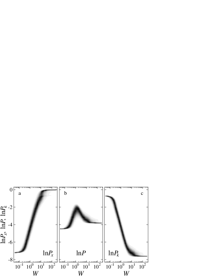
Figure 2: Distributions of the logarithms of the inverse participation ratio for 50 disorder realizations in (a) real space, (b) phase space, and (c) momentum space as a function of the disorder strength $W$ for a one-dimensional system of length $L=2048$.

In the limit of very strong disorder, the states are localized on a single site in real space and uniformly distributed over momentum space. This leads to the limiting values $P_{x}(\infty)=1$ and $P_{k}(\infty)=L^{-d}$. In phase space one has to account for the finite width of the Husimi function and thus finds $P(\infty)=L^{-d/2}$. For $d=1$, these values can be checked against the data shown in Fig. 2. Starting from this limit, with decreasing disorder two energetically almost degenerate states become coupled via the finite hopping matrix element $t$. For these states $P_{x}$ is reduced to $1/2$ while $P_{k}$ is enhanced by a factor of $3/2$. As already discussed above, it is the latter which dominates the behavior in phase space.

In the opposite limit $W\to 0$, the real wave functions in $d=1$ contain equal contributions from degenerate plane waves of momenta $k$ and $-k$. This implies $P_{k}(0)=1/2$ and $P_{x}(0)=2/3L$. In phase space, the finite width of the Husimi function leads to $P(0)=1/2L^{1/2}$. In higher dimensions, however, degeneracies occur and render the behavior for $W\to 0$ more complex. Nevertheless, as a function of system size, $P_{x}$ and $P$ scale as $L^{-d}$ and $L^{-d/2}$, respectively. A more detailed discussion will be given elsewhere wobstxx .

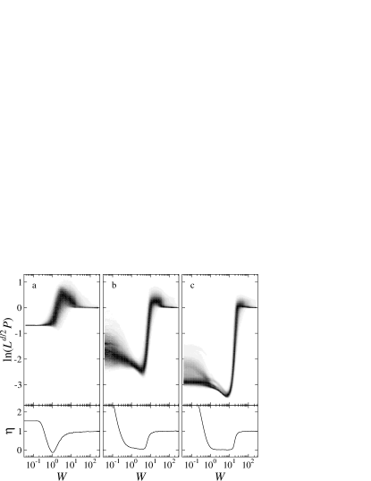
Figure 3: Distributions of the logarithms of the inverse participation ratio in phase space (top) and $\eta$ defined in Eq. (6) (bottom) are shown as a function of disorder strength $W$ for (a) $d=1,L=128$, (b) $d=2,L=64$, and (c) $d=3,L=20$. The distributions are based on 250, 20, and 20 disorder realizations, respectively.

The upper part of Fig. 3 shows the distributions of the logarithm of $P$ for dimensions $d=1,2,$ and 3 and system sizes $L=128,64,$ and 20, respectively. For better comparison the data have been scaled with the length dependence $L^{-d/2}$, being valid in the limits $W\to 0$ and $\infty$.

The most striking difference between the one-dimensional case and higher dimensions consists in the behavior of the inverse participation ratio for weak disorder. For $d=1$, the average inverse participation ratio increases with disorder strength and eventually goes through a maximum. The overall behavior can be understood as a crossover from a regime dominated by real space properties to one dominated by momentum space.

In contrast, in $d\geq 2$ the average inverse participation ratio initially decreases. This implies a spreading of the Husimi function beyond the broadened stripes present for weak disorder (cf. Fig. 1a). On the other hand, the behavior at strong disorder is governed by the same mechanism as for the one-dimensional case, which implies an increase of the inverse participation ratio with decreasing disorder. The two regimes are joined by a short interval of disorder strengths where the Husimi function contracts strongly as disorder is increased.

The distributions of $P$ depicted in Fig. 3 behave similarly for $d=2$ and 3. However, the pertinent scaling argument for Anderson localization abrah79 predicts a phase transition only in dimensions higher than two. Unfortunately, in $d=3$ numerical constraints prevent us from performing a finite size scaling, which would allow to distinguish the form of the jumps of $P$ in $d=2$ and 3 in the thermodynamic limit $L\to\infty$.

The main difference between the behavior in $d=1$ and $d\geq 2$, the appearance of a minimum in the inverse participation ratio $P$, can be associated with the existence of a diffusive regime in $d\geq 2$. While in $d=3$ a diffusive regime appears even in the thermodynamic limit, in $d=2$ it is present for systems of finite size when the system size exceeds the mean free path but not the localization length. It is suggestive to conclude that diffusive motion is associated with a large spread in phase space and thus with the minimum observed in the inverse participation ratio.

To substantiate this idea, we compare our results to energy level statistics. In the diffusive regime the energy spacing distribution $p(s)$ is close to the Wigner-Dyson distribution $p_{W}(s)=\frac{1}{2}\pi s\exp(-\pi s^{2}/4)$. In contrast, in the localized regime, $p(s)$ approaches the Poissonian statistics $p_{P}(s)=\exp(-s)$. To quantify the form of the distribution we evaluate

$$\eta=\frac{\int_{0}^{b}ds(p(s)-p_{W}(s))}{\int_{0}^{b}ds(p_{P}(s)-p_{W}(s))}$$ (6)

which is particularly sensitive to level repulsion. Here, $b=0.4729\dots$ refers to the first crossing point of the distributions $p_{W}(s)$ and $p_{P}(s)$. According to its definition, $\eta=1$ for a Poissonian spacing distribution and $\eta=0$ for a Wigner-Dyson spacing distribution.

In the lower part of Fig. 3, $\eta$ is shown as a function of the disorder strength. For weak disorder, $\eta$ exceeds 1 because of non-universal level statistics appearing in regular geometries in the ballistic regime. For strong disorder one finds Poissonian statistics as expected for the localized regime. At intermediate disorder strengths in $d=1$, $\eta$ exhibits a minimum due to level repulsion, but no proper diffusive regime exists. On the other hand, for finite size systems in $d=2$, an extended region is present, where the level statistics is close to that predicted by random matrix theory. This property is commonly used to identify a region of diffusive dynamics. For $d=3$ the diffusive region survives even in the thermodynamic limit $L\to\infty$.

Fig. 3 clearly shows that the decrease of the inverse participation ratio $P$ is related to a plateau of $\eta$ at values close to zero. Using the spreading of the states in phase space as an indicator for diffusive behavior is therefore consistent with the results from level statistics. For $d=3$, a comparison between $\eta$ and the distribution of $P$ even allows to identify the ballistic regime for weak disorder, where the inverse participation ratio essentially remains constant.

In conclusion, we have shown that phase space properties represent a new tool to describe disordered systems for arbitrary disorder strength. The inverse participation ratio $P$ in phase space provides information, which could not be obtained from the corresponding quantities $P_{x}$ in real space and $P_{k}$ in momentum space. It is only the first quantity which captures the appearance of a diffusive regime in two and higher dimensions. Given our demonstration that the physics in phase space is able to provide new insight into the dynamics of disordered systems, these concepts likely will also make a valuable contribution towards understanding the challenging problem of the combined effects of interaction and disorder in few-body systems.

- (1) A. D. Mirlin, Phys. Rep. 326, 259 (2000).
- (2) E. Abrahams, P. W. Anderson, D. C. Licciardello, and T. V. Ramakrishnan, Phys. Rev. Lett. 42, 673 (1979).
- (3) P. A. Lee and T. V. Ramakrishnan, Rev. Mod. Phys. 57, 287 (1985).
- (4) P. W. Anderson, Phys. Rev. 109, 1492 (1958).
- (5) B. Kramer and A. MacKinnon, Rep. Prog. Phys. 56, 1469 (1993) and references therein.
- (6) K. Husimi, Proc. Phys. Math. Soc. Jpn. 22, 264 (1940).
- (7) K. E. Cahill and R. J. Glauber, Phys. Rev. 177, 1882 (1969).
- (8) A. Wehrl, Rep. Math. Phys. 16, 353 (1979).
- (9) B. Mirbach and H. J. Korsch, Phys. Rev. Lett. 75, 362 (1995).
- (10) S. Gnutzmann and K. Życzkowski, eprint quant-ph/0106016.
- (11) T. Gorin, H. J. Korsch, and B. Mirbach, Chem. Phys. 217, 145 (1997).
- (12) S. Fishman, D. R. Grempel, and R. E. Prange, Phys. Rev. Lett. 49, 509 (1982).
- (13) D. Weinmann, S. Kohler, G.-L. Ingold, and P. Hänggi, Ann. Phys. (Leipzig) 8, SI277 (1999).
- (14) There are subtle differences between entropies and inverse participation ratios as was discussed in real space in I. Varga and J. Pipek, J. Phys.: Condens. Matter 6, L115 (1994).
- (15) D. J. Thouless, Phys. Rep. 13, 93 (1974).
- (16) P. Leboeuf and A. Voros, J. Phys. A 23, 1765 (1990).
- (17) A. Wobst, G.-L. Ingold, P. Hänggi, and D. Weinmann (unpublished).