[

Finite-Temperature Phase Diagram of Hard-Core Bosons in Two Dimensions

Abstract

We determine the finite-temperature phase diagram of the square lattice hard-core boson Hubbard model with nearest neighbor repulsion using quantum Monte Carlo simulations. This model is equivalent to an anisotropic spin-1/2 $XXZ$ model in a magnetic field. We present the rich phase diagram with a first order transition between solid and superfluid phase, instead of a previously conjectured supersolid and a tricritical end point to phase separation. Unusual reentrant behavior with ordering upon increasing the temperature is found, similar to the Pomeranchuk effect in ³He.

] A nearly universal feature of strongly correlated systems is a phase transition between a correlation-induced insulating phase with localized charge carriers, to an itinerant phase. High temperature superconductors [1], manganites [2] and the controversial two dimensional (2D) “metal-insulator-transition” [3] are just a few examples of this phenomenon. The 2D hard-core boson Hubbard model provides the simplest example of such a transition from a correlation-induced charge density wave insulator near half filling to a superfluid (SF). It is a prototypical model for preformed Cooper pairs [4], of spin flops in anisotropic quantum magnets [5, 6], of SF Helium films[7] and of supersolids [8, 9].

In simulations on this model, which does not suffer from the negative sign problem of fermionic simulations, we can investigate some of the pertinent questions about such phase transitions: what is the order of the quantum phase transitions in the ground state and the finite temperature phase transitions? Are there special points with dynamically enhanced symmetry [10]? Can there be coexistence of two types of order (such as a supersolid – coexisting solid and superfluid order)? Answers to these questions provide insight also for the other problems alluded to above.

The Hamiltonian of the hard-core boson Hubbard model we study is

$$H= - t\sum_{\langle{\bf i},{\bf j}\rangle}(a_{{\bf i}}^{\dagger}a_{{\bf j}}+a_{{\bf j}}^{\dagger}a_{{\bf i}})+V\sum_{\langle{\bf i},{\bf j}\rangle}n_{{\bf i}}n_{{\bf j}}-\mu\sum_{\bf i}n_{\bf i},$$ (1)

where $a_{\bf i}^{\dagger}$ $(a_{\bf i})$ is the creation (annihilation) operator for hard-core bosons, $n_{\bf i}=a_{\bf i}^{\dagger}a_{\bf i}$ the number operator, $V$ the nearest neighbor Coulomb repulsion and $\mu$ the chemical potential. This model is equivalent to an anisotropic spin-1/2 $XXZ$ model with $J_{z}=V$ and $|J_{xy}|=2t$ in a magnetic field $h=2V-\mu$. The zero field (and zero magnetization $m_{z}=0$) case of the spin model corresponds to the half filled bosonic model (density $\rho=\langle m_{z}\rangle=1/2$) at $\mu=2V$. Throughout this Letter we will use the bosonic language, and refer to the corresponding quantities in the spin model where appropriate. Due to the absence of efficient Monte Carlo algorithms for classical magnets in a magnetic field there are still many open questions even in the classical version of this model, which was only studied by a local update method [11].

In Fig. 1 we show the ground-state phase diagram [6, 9, 12]. For dominating chemical potential $\mu$ the system is in a band insulating state ($\rho=0$ and $\rho=1$ respectively), while it shows staggered checkerboard charge order ($\rho=1/2$) for dominating repulsion $V$. These solid phases are separated from each other by a SF. Earlier indications for a region of supersolid phase between checkerboard solid and SF phase turned out to be due to phase separation at this transition which is of first order at $T=0$ [6, 9, 12].

FIG. 1.: Ground-state phase diagram of the hard-core boson Hubbard model. The dashed line indicates the cut along which we calculated the finite-temperature phase diagram shown in Fig. 2.

All of these phases extend to finite temperatures. On the strong repulsion side the hard-core boson Hubbard model is equivalent to an antiferromagnetic Ising model at $t=0$ and the insulating behavior extends up to a finite-temperature phase transition of the Ising universality class ($T_{c}\approx 0.567V$ at half filling). In case of zero repulsion the system is equivalent to an XY model in a magnetic field and the SF extends up to a transition of Kosterlitz Thouless (KT) type at finite temperature. The point $V=2t$ and $\mu=2V$ is also of special interest, it corresponds to the Heisenberg point in the spin model and has an enlarged $O(3)$ symmetry, with long range order only at zero temperature in 2D [13].

We focus our attention on the finite-temperature phase diagram in the vicinity of the first order quantum phase transition separating the SF and solid ground states away from the Heisenberg point. It is instructive to first consider the three dimensional (3D) version of this model, with a similar ground-state phase diagram. There, Fisher and Nelson [10] determined that the first order line terminates at a finite-temperature bicritical point at which the transition temperatures of the solid and SF phases meet. This bicritical point has a dynamically enhanced $O(3)$ symmetry – the symmetry of the Hamiltonian is only $O(2)$.

This feature alone dictates that despite the similar ground-state phase diagrams, the finite-temperature phase diagrams have to be very different in 2D, as an $O(3)$ critical point in 2D can exist only at zero temperature [13]. Even with the absence of a supersolid in the ground state several alternative scenarios are still plausible: (i) the bicritical point could be pulled down to zero temperature, and the transition temperatures $T_{KT}$ and $T_{c}$ approach zero temperature without a direct phase transition between SF and solid at finite temperatures, (ii) a supersolid phase could exist at finite temperatures, although it is absent in the ground state, or (iii) the phase transition lines meet at finite temperature, but without dynamically enhanced symmetries.

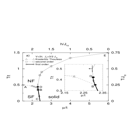
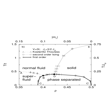
FIG. 2.: Phase diagrams at $V=3t$ as function of a) $\mu$ and $T$ and b) $\rho$ and $T$. The arrow in the inset of the upper panel denotes an upper bound for the critical $\mu$ at $T=0.5t$. The error bars of the triangles are strict bounds for the KT transition. The right and upper axis show the parameters in the spin language. The solid circle and square denote qualitatively where we expect the critical points to be. Lines are guides to the eye.

In order to decide between these possibilities and determine the finite-temperature phase diagram we use quantum Monte Carlo simulations, employing a variant [14, 15] of the worm algorithm [16] in the stochastic series expansion (SSE) representation [14]. The simulations were performed in the grand canonical ensemble using lattices up to size $96\times 96$ and do not suffer from any systematic error apart from finite size effects. In contrast to the loop algorithm [17] the worm algorithm, while not as efficient at half filling (a spin model in zero magnetic field), remains effective away from half filling (in a finite field), where the loop algorithm slows down exponentially.

From now on we will restrict our discussion to $V=3t$, which corresponds to the dashed line in Fig. 1. We present the finite-temperature phase diagram for this representative value in Fig. 2. Due to particle-hole symmetry it is sufficient to show densities up to $1/2$ and chemical potentials up to $\mu=2V=6t$. We find that scenario (iii) is realized: the first order phase transition extends to a tricritical point (D) at around $T_{3}\approx 0.4t$, where it meets with the second order melting transition of the solid. The KT transition temperature $T_{KT}$ of the SF meets the first order line at a lower temperature (B) – in contrast to the 3D case, where all the three lines meet at the same bicritical point (B$=$D) with enhanced $O(3)$ symmetry. We want to emphasize one unusual feature before discussing in detail how the phase diagram was determined: there is reentrant behavior in the vicinity of the tricritical point (D) and the system melts upon decreasing the temperature at constant chemical potential.

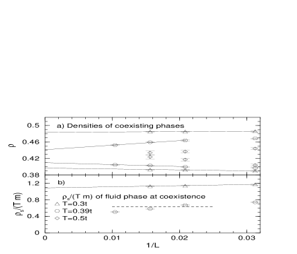
FIG. 3.: a) Finite size scaling of the coexistence densities at different temperatures, demonstrating the first order nature of the phase transition at $T\leq 0.39t$. b) Finite size scaling of the SF density $\rho_{s}$ at different temperatures, showing that the first order transition is between a solid and SF at low temperatures, and between a solid and normal fluid at higher temperatures. The dashed line shows the value of $\rho_{s}/(Tm)$ at a KT transition. All simulations are done at $V=3t$.

The first order phase transition is characterized by a finite jump $\Delta\rho$ in the density. As discussed in Ref. [12], where we present the ground-state phase diagram, two peaks can be observed in the density distribution at the critical chemical potential. Since a two-peak structure can also be seen at a second order transition in a finite system, a careful finite size scaling analysis is needed. Figure 3a shows the finite size scaling of the densities of the two coexisting phases. For $T\leq 0.39t$ the jump $\Delta\rho$ remains finite under extrapolation, thus confirming the first order nature up to this temperature (line from C to D in Fig. 2), while it scales to zero for $T\geq 0.45t$, an indication for a second order transition (line from D to E). Additionally we have checked the finite size scaling of the fourth order cumulant ratio $C_{4}=1-\langle m_{s}^{4}\rangle/3\langle m_{s}^{2}\rangle^{2}$, of the staggered charge order parameter $m_{s}$ in the solid phase. Consistency with the expected size independent universal value of the Ising universality class $C_{4}^{c}=0.6106900(1)$ [18] at the transition confirms the second order nature. We have thus determined that the first order transition extends up to a critical point (D) at a temperature larger than $0.39t$ and smaller than $0.45t$. In the next paragraph we show that the critical point where the KT line meets the first order line (point B) is below $0.39t$. Therefore the end point D of the first order line is a tricritical point.

The KT transition temperatures $T_{KT}$ (line from A to B in Fig. 2) can be determined using the SF number density $\rho_{s}=(mT/2)\langle W_{x}^{2}+W_{y}^{2}\rangle$ [19]. Here $W_{x}$ and $W_{y}$ are the winding numbers of the world lines in $x$ and $y$ direction respectively, and $m=1/(2t)$ is the mass of a boson. For system size $L=\infty$, $\rho_{s}$ has a universal value at $T_{KT}$, $\rho_{s}(T_{KT})=(2/\pi)mT_{KT}$, while it is always larger than this universal value for $T<T_{KT}$. At $T=T_{KT}$, $\rho_{s}$ jumps from the universal value to zero and we have $\rho_{s}(T)=0$ for all $T>T_{KT}$. However, for finite $L$, $\rho_{s}$ is nonzero at all $T$ and the finite size corrections of $\rho_{s}$ at $T=T_{KT}$ are given by [19] $\rho_{s}\pi=2mT_{KT}(1+\{2\log[L/L_{0}(T_{KT})]\}^{-1})$. Although these finite size corrections are known to be notoriously difficult, we can obtain strict upper and lower bounds for $T_{KT}$ by plotting $1/(\pi\rho_{s}/mT-2)-\log(L)$ as function of $\log L$. As $L$ is increased, this quantity converges to the constant $(-\log L_{0})$ at $T_{KT}$ and diverges to $\pm\infty$ for $T>T_{KT}$ and $T<T_{KT}$, respectively [20]. The error bars we obtain using this method are reliable and small enough for our purposes.

To investigate how the KT transition line meets the phase separation line we perform canonical measurements of the SF density $\rho_{s}$ at the density $\rho_{f}$ of the fluid on this coexistence line. In Fig. 3b we show the finite size scaling of $\rho_{s}(\rho_{f})$. At low temperatures $T=0.3t$ $\rho_{s}$ of the SF at the coexistence line is well above the universal value for a KT transition. Therefore the transition between SF and solid at temperatures $T\leq 0.3t$ does not include a KT transition. The system remains SF right up to a direct first order phase transition from the SF to the solid. At $T=0.39t$ on the other hand, $\rho_{s}$ as a function of the system size $L$ drops below the universal value and should scale to zero according to [21]. There is thus a first order transition from solid to normal fluid at $T=0.39t$ and the KT line has to meet the first order line at a finite temperature between $0.3t$ and $0.39t$.

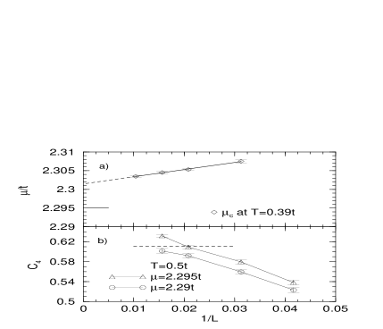
FIG. 4.: a) Finite size scaling of the critical chemical potential $\mu_{c}$ at $T=0.39t$. The horizontal line is an upper bound for the critical chemical potential at $T=0.5t$. b) Finite size scaling of the fourth order cumulant $C_{4}$ at $T=0.5t$ for different chemical potentials. The horizontal line is the universal value of $C_{4}$ at the Ising critical point. All simulations are done at $V=3t$.

As can be seen in Fig. 2, the checkerboard solid is melting in a first order transition to a SF upon decreasing the temperature around $\mu\simeq 2.35t$. Even more special is the melting to a normal fluid in the vicinity of the tricritical point (D) both upon increasing or decreasing the temperature. To proof this reentrant behavior, we first determine the critical chemical potential $\mu_{c}(T=0.39t)$ of the first order transition at $T=0.39t$. We then show that $\mu_{c}(T=0.5t)<\mu_{c}(T=0.39t)$ On a finite system we define $\mu_{c}$ as the chemical potential where there is an equal probability to be in the solid and fluid phase (equal peak areas in the density probabilities). Performing a finite size extrapolation (Fig. 4a) we obtain $\mu_{c}(0.39t)=2.3015(10)t$. Next we calculate the upper bound for the critical chemical potential $\mu_{c}(T)$ at $T=0.5t$. Observing that the fourth order cumulant ratio $C_{4}$ scales above the universal critical value $C_{4}^{c}$ at $\mu=2.295t$ (Fig. 4b), we thus have $\mu_{c}(T=0.5t)<2.295t$. As $\mu_{c}(T=0.5t)<\mu_{c}(T=0.39t)$ we have pinpointed reentrant behavior where the solid melts to a normal fluid both when increasing and decreasing the temperature.

To summarize, we have investigated the finite-temperature phase diagram of the hard-core boson Hubbard model with nearest neighbor repulsion using quantum Monte Carlo simulations. The first order phase transition in the ground state between SF and solid phases extends to finite temperatures and turns into a second order melting line of the solid phase at a finite-temperature tricritical point. As the KT line meets the first order line at a lower temperature, we have a qualitatively different phase diagram than in 3D [10], where there is a bicritical point with dynamically enhanced $O(3)$ symmetry.

We expect this phase diagram, obtained for a representative value of $V=3t$, to be valid also for other couplings $V>2t$. On approaching the Heisenberg point $V=2t$ the temperature scale of all the transitions drops to zero. In the other limit $t/V\rightarrow 0$, we approach the antiferromagnetic Ising model. The KT transition temperatures $T_{KT}$ and the tricritical point $T_{3}$ should scale with $t$, since in the Ising model the phase transition is first order at zero temperature, but second order at any finite temperature [22], consistent with $T_{3}/V\sim t/V\rightarrow 0$.

The melting line of the solid shows several unusual features. As a function of chemical potential there are three different phase transitions: at low temperatures the melting transition is first order into a SF. At intermediate temperatures the melting transition is still first order, but to a normal fluid, while it is a second order transition to a normal fluid at even higher temperatures.

There is reentrant behavior in the vicinity of the tricritical point: as a function of increasing temperature there are three phase transitions: first the SF turns into a normal fluid. Upon increasing the temperature further this normal fluid solidifies, and finally melts again. The reason for this reentrant behavior is conjectured to be a large entropy of the weakly interacting vacancies (or interstitials at $\rho>1/2$) in the solid, larger than the entropy of the normal fluid. Such an ordering transition upon increasing temperature is rare but has been observed before, e.g. in the bcc Ising antiferromagnet [23].

Finally, we want to mention the striking qualitative similarity of the presented phase diagram to those of fermionic ³He and bosonic ⁴He in two dimensions. In ³He there is also a reentrant melting line (the Pomeranchuk effect [24]) and a SF phase at low temperatures [25]. In ³He however the large entropy of the solid is due to the nuclear spin degrees of freedom and the effect even more pronounced. In ⁴He films, the solid phase melts to a SF in a small range for the pressure upon decreasing the temperature [26], like in our phase diagram where there is a direct transition form SF to solid for constant values of $\mu$ around $\mu\simeq 2.35t$. Note that in our phase diagram we have pinned down the even more subtle effect of a reentrant melting line between solid and normal fluid.

We wish to thank G.G. Batrouni and D.M. Ceperley for stimulating discussions. The simulations were performed on the Asgard Beowulf cluster at ETH Zürich, employing the Alea library for Monte Carlo simulations [27]. G.S., S.T. and M.T. acknowledge support of the Swiss National Science Foundation.

REFERENCES

- [1] J.G. Bednorz and K.A. Müller, Z. Phys. B 64, 189 (1986).
- [2] E. Dagotto et al., Phys. Rep. 344, 1 (2001).
- [3] E. Abrahams et al., Rev. Mod. Phys. 73, 251 (2001).
- [4] T. Siller et al., Phys. Rev. B 63, 195106 (2001); A. Dorneich et al., Phys. Rev. Lett. 88, 057003 (2002); A.P. Kampf and G.T. Zimanyi, Phys. Rev. B 47, 279 (1992); G.G. Batrouni et al., Phys. Rev. B 48, 9628 (1993); M. Cha et al., Phys. Rev. B 44, 6883 (1991); E.S. Sørensen et al., Phys. Rev. Lett. 69, 828 (1992).
- [5] A. van Otterlo et al., Phys. Rev. B 52, 16176 (1995).
- [6] M. Kohno and M. Takahashi, Phys. Rev. B 56, 3212 (1997).
- [7] G.T. Zimanyi et al., Phys. Rev. B 50, 6515 (1994).
- [8] G.G. Batrouni et al., Phys. Rev. Lett. 74, 2527 (1995); R.T. Scalettar et al., Phys. Rev. B 51, 8467 (1995).
- [9] G.G. Batrouni and R.T. Scalettar, Phys. Rev. Lett. 84, 1599 (2000).
- [10] M. E. Fisher and D. R. Nelson, Phys. Rev. Lett. 32, 1350 (1974).
- [11] D.P. Landau and K. Binder, Phys. Rev. B 24, 1391 (1981).
- [12] F. Hebert et al., Phys. Rev. B 65, 014513 (2002).
- [13] N.D. Mermin and H. Wagner, Phys. Rev. Lett. 17, 1133 (1966).
- [14] A.W. Sandvik, Phys. Rev. B 59, 14157 (1999).
- [15] A. Dorneich and M. Troyer, Phys. Rev. E 64, 066701 (2001).
- [16] N.V. Prokof’ev et al., Sov. Phys. - JETP 87, 310 (1998).
- [17] H.G. Evertz et al., Phys. Rev. Lett. 70, 875 (1993); B. B. Beard and U.-J. Wiese, Phys. Rev. Lett. 77, 5130 (1996).
- [18] G. Kamieniarz and H. Blöte, J. Phys. A: Math Gen. 26, 201 (1993).
- [19] K. Harada and N. Kawashima, J. Phys. Soc. Jpn. 67, 2768 (1998); Phys. Rev. B 55, R11949 (1997).
- [20] M. Troyer and S. Sachdev, Phys. Rev. Lett. 81, 5418 (1998).
- [21] D.R. Nelson and J.M. Kosterlitz, Phys. Rev. Lett. 39, 1201 (1977).
- [22] S. Todo and M. Suzuki, Int. J. Mod. Phys. C 6, 811 (1996); H. Blöte and X. Wu, J. Phys. A: Math. Gen. 23, L627 (1990).
- [23] D.P. Landau, Phys. Rev. B 16, 4164 (1977).
- [24] I. Pomeranchuk, Zh. Eksperim. i Teor. Fiz. 20, 919 (1950); Yu. D. Anufriyev, JETP Letters 1, 155 (1965).
- [25] See, e.g. M.M. Salomaa and G.E. Volovik, Rev. Mod. Phys. 59, 533 (1987).
- [26] M.C. Gordillo and D.M. Ceperley, Phys. Rev. B 58, 6447, (1998).
- [27] M. Troyer et al., Lec. Notes Comp. Sci. 1505, 191 (1998).