Superfluidity and Superconductivity in Double-Layered Quantum Hall state

Abstract

We discuss and review the basic physics that leads to superfluidity/superconductivity in certain quantum Hall states, in particular the so-called double-layered $(mmm)$ state. In the $K$-matrix description of the quantum correlation in quantum Hall states, those states with det$(K)=0$ contain a special correlation that leads to superfluidity/superconductivity. We propose a four-terminal measurement to test the DC Josephson-like effect in interlayer tunneling, so that the issue of superfluidity/superconductivity in the $(mmm)$ states can be settled experimentally.

Almost 10 years ago we predicted[1, 2, 3, 4] that under certain circumstances a double layered quantum Hall system would exhibit the physics of superfluidity/superconductivity. Recently, this apparently surprising and somewhat counter-intuitive prediction was verified dramatically by Eisenstein et al[5] in a form of (two-terminal) DC Josephson-like effect for interlayer tunneling.

Historically, the gapless mode in the $(111)$ double layered quantum Hall state was first discovered by Fertig[6]. Later, the effect of interlayer tunneling was included[7, 8]. However, superfluidity and superconductivity were not discussed in these earlier work. In Ref. [1, 2], we discovered and identified the spontaneously broken $U(1)$ symmetry in the $(mmm)$ states and emphasized the resulting superfluidity and superconductivity. The properties we discussed include the Kosterlitz-Thouless transition, the zero resistivity in the counter-current flow, the DC/AC Josephson-like effect in interlayer tunneling, as well as the gapless superfluid mode. Some of these results were obtained later using an isospin approach for the special $m=1$ case[9].

We stressed that the Josephson-like effect we predicted in the $(mmm)$ state differ in some crucial respects from the Josephson effect for superconductor junction[2]. The critical current for the $(mmm)$ state is proportional to the electron tunneling amplitude, rather than the square of the tunneling amplitude as in the DC Josephson effect between superconductors. More strikingly, the Josephson frequency in the AC Josephson-like effect for the $(mmm)$ states is given by [2]

$$f_{J}^{*}=eV/h,$$ (1)

half of the standard Josephson frequency $f_{J}=2eV/h$ in the AC Josephson effect between superconductors.

There appears to be some confusion and disagreement in the literature concerning the superfluidity/superconductivity in the $(mmm)$ states. It has been argued in Ref. [10] that “although gapless out-of-phase modes associated with a spontaneously broken continuous symmetry can occur in double-layer systems they do not imply superfluid behavior”. In particular, the DC Josephson-like effect in the interlayer tunneling remain a controversial issue[10, 11]. Since the physics underlying the superfluidity/superconductivity in double-layered quantum Hall system is both fundamental and profound, we would like to clarify and review some of the basic principles. Some of what we say here can be found in one form or another in our original paper and in various reviews[12, 13] we wrote. Still, we hope that our presentation here will help to shed light on the basic physics.

In this paper, we will propose a four-terminal set-up to test the DC Josephson-like effect experimentally. We hope that future experiments will clarify the controversy on the DC Josephson-like effect and the superfluidity/superconductivity in the $(mmm)$ states.

For conceptual clarity, our discussion here will be entirely at zero temperature.

1 A dual description of the superfluid

As was emphasized by Feynman[16] among others, the physics of superfluidity lies not in the presence of gapless excitations, but in the paucity of gapless excitations. After all, the Fermi liquid has a continuum of gapless modes. Indeed, consider a gas of free bosons at zero temperature. We can give a momentum $\hslash\vec{k}$ to any given boson at the cost of only $\hslash\vec{k}^{2}/2m$ in energy. There exist many low energy excitations in a free boson system. But as soon as a short-ranged repulsion is turned on between the bosons, a boson moving with momentum $\vec{k}$ would affect all the other bosons. A density wave is set up as a result. As Bogoliubov and others have taught us, the density wave has energy $\varpropto k$. The gapless mode has gone from quadratically dispersing to linearly dispersing. There are far fewer low energy excitations. Specifically, the density of states $N(E)\varpropto k^{D-1}(\frac{dk}{dE})$ goes from $N(E)\varpropto$ constant to $N(E)\varpropto E$ at low energies. Here we have set the dimension of space $D$ to 2.

If we accept the point of view that the key ingredient of superfluidity is the existence of only one mode of gapless excitations, then we can use this picture to give a semi-quantitative description of superfluid. As the above discussion makes clear, the linearly dispersing gapless mode is a density wave. As Landau first proposed, such a density fluctuation can be described hydrodynamically. The kinetic energy density is then simply given by the square of the current density $\vec{j}$, while the potential energy density is given by $(\delta\rho)^{2}$ where $\delta\rho$ represents the deviation of number density $\rho$ from some mean density $\rho_{0}$. Thus, suppressing some constant factors (which we can set to unity by a suitable choice of spacetime units), we have the effective Lagrangian for the superfluid $\mathcal{L}=\vec{j}^{2}-(\delta\rho)^{2}+\cdots$ where as always in an effective Lagrangian description the $(\cdots)$ represent physics that are not important at low energy and momentum. Suppressing the $\delta$ on $\delta\rho$ and using the relativistic notation $j^{\mu}=(\rho,\vec{j})$ we can write

$$\mathcal{L}=-j^{\mu}j_{\mu}+\cdots$$ (2)

A crucial physical principle underlying a hydrodynamic description is of course current conservation $\frac{\partial\rho}{\partial t}-\vec{\triangledown}\vec{j}=0,$ or in relativistic notation

$$\partial_{\mu}j^{\mu}=0.$$ (3)

This conservation equation is solved by writing

$$j^{\mu}=\frac{1}{2\pi}\varepsilon^{\mu\nu\lambda}\partial_{\nu}a_{\lambda}$$ (4)

We recognize the symbol $a_{\lambda}$ as representing a gauge potential since the transformation

$$a_{\lambda}\rightarrow a_{\lambda}+\partial_{\lambda}\Lambda$$ (5)

leaves the physical current $j^{\mu}$ and hence physics unchanged. The relation (4) is an example of a duality relation.

Upon substituting (4) into (2) we obtain the effective Lagrangian in terms of the gauge potential $a_{\lambda}$

$$\mathcal{L}_{superfluid}=-\frac{1}{8\pi^{2}}f^{\mu\nu}f_{\mu\nu}+\cdots$$ (6)

where $f_{\mu\nu}=\partial_{\mu}a_{\nu}-\partial_{\nu}a_{\mu}$. We refer to (6) as the Maxwell Lagrangian since it has the same form as the Lagrangian introduced by Maxwell to describe electromagnetism.

We could have described the gapless linearly dispersing mode by the equation of motion $\partial_{\mu}f^{\mu\nu}=0$ and thus gone to (6) directly. However, it would have been unclear why we would need a spin 1 field to describe one gapless mode, even though it is true that in $(2+1)$ dimensional spacetime a spin $1$ field contains only one physical degree of freedom. This gapless mode is in fact a Nambu-Goldstone boson. Since the only locally conserved quantity in our interacting Bose gas is the number density $\rho$ associated with a global $U(1)$ symmetry, this global symmetry must be spontaneously broken. This is indeed so as the number of bosons in the $\vec{k}=0$ ground state is a finite fraction of the total number of bosons.

The physics of gapless mode is particularly transparent in Bogoliubov’s calculation. Let $a_{0}$ and $a_{0}^{\dagger}$ be the annihilation and creation operators for bosons in the $\vec{k}=0$ non-interacting ground state. In the interaction term $\sum\limits_{k,p,q}G(a_{k}^{\dagger}a_{p}^{\dagger}a_{q}a_{k+p-q})$ in the Hamiltonian $H$ Bogoliubov replaces $a_{0}$ and $a_{0}^{\dagger}$ by $c-$numbers $<a_{0}>=<a_{0}^{\dagger}>=u,$ thus giving schematically

$$H\sim\sum_{k\neq 0}Gu^{2}(a_{k}^{\dagger}a_{k}+a_{-k}^{\dagger}a_{-k}+a_{k}^{\dagger}a_{-k}^{\dagger}+a_{-k}a_{k})+\sum_{k}\frac{k^{2}}{2m}a_{k}^{\dagger}a_{k}$$ (7)

Clearly, we get a gapless mode since up to an additive constant the first term can be written as $\sum_{k\neq 0}Gu^{2}(a_{k}^{\dagger}+a_{-k})(a_{k}+a_{-k}^{\dagger})$ and so $a_{k}^{\dagger}-a_{-k}$ creates a gapless excitation of momentum $\vec{k}.$ The crucial point is that $<a_{0}>=<a_{0}^{\dagger}>\neq 0$ and not merely $<a_{0}^{\dagger}a_{0}>\neq 0$ : in that case we would only get a gapped mode with energy $(2Gu^{2}+\frac{k^{2}}{2m})$.

Formally, the $U(1)$ symmetry breaking can be described by a field theoretic representation of the boson gas

$$\mathcal{L}=\partial\Phi^{\dagger}\partial\Phi-V(\Phi^{\dagger}\Phi)$$ (8)

A superfluid is defined as a fluid in which $<\Phi>=we^{i\theta}$ does not vanish. As is well known, this breaks the global $U(1)$ symmetry $\Phi\rightarrow e^{i\alpha}\Phi$ of the Lagrangian $\mathcal{L}$. In this language, it is possible to describe the gapless linearly dispersing mode by a scalar field and to write

$$\mathcal{L}_{superfluid}=\frac{c}{2}(\partial_{\mu}\theta)^{2}+\cdots$$ (9)

where the phase field is the phase of the field $\Phi$. We note that the Lagrangian (6) and (9) describe the same superfluid mode and the two theories are dual to each other.

2 Quantum Hall Fluid

The Hall fluid is another highly coherent quantum state. To see how the low energy effective theories of the Hall fluid and of the superfluid differ from each other, we need to understand the correlations in the quantum Hall ground state. The simplest kind of Hall fluid with filling fraction $\nu=1/k$ is described by the ground state wave function proposed by Laughlin

$$\Psi\sim\prod\limits_{i,j}(z_{i}-z_{j})^{k}$$ (10)

with $k$ an odd integer. This highly non-trivial wave function captures the strong quantum correlation between particles. As electron $i$ goes around electron $j$ the wave function acquires a factor $e^{2i\pi k}.$ As is well known but still worth emphasizing, the essential physics involved is purely quantum in character and has no classical counterpart.

This quantum phase correlation is the same as in the Aharonov-Bohm effect and so the particles in (10) can be regarded as carrying both charge and flux associated with some gauge field. As was shown by Wilczek and Zee[14], this phase correlation can be expressed mathematically as a Hopf term which in turn can be generated by a Chern-Simons term in the gauge action. The phase correlation can also be viewed as a density-current interaction.

The origin of the Hopf and Chern-Simon terms can be easily understood in physical terms within the context of this discussion. When electron $i$ goes around electron $j$, we have a current $\vec{j}$ around a charge density $\rho$ (as before, we drop the $\delta$), and so the action $S$ should contain a non-local term of the form $\sim$ $\int d^{3}x$ $\int d^{3}x^{\prime}$ $\rho(x)\vec{K}(x-x^{\prime})\vec{j}(x^{\prime})$ in addition to the terms in (2). Such a term describes a non-local current-density interaction. The kernel $\vec{K}$ can be determined from basic principles. Rotational invariance and scale invariance fix this term to be $S_{Hopf}$ $\sim$ $\int d^{3}x$ $\int d^{3}x^{\prime}$ $k\rho(x)\frac{1}{|x-x^{\prime}|}\vec{\triangledown}\times\vec{j}(x^{\prime})$ or in relativistic form

$$S_{Hopf}\sim k\int d^{3}x\varepsilon^{\mu\nu\lambda}j_{\mu}\frac{1}{\partial^{2}}\partial_{\nu}j_{\lambda}.$$ (11)

We have scale invariance because we know that the phase factor $e^{i(2\pi m)}$ does not depend on the separation between particles $i$ and $j$: there is no characteristic distance in the quantum phase correlation. Note that the cross product $\vec{\triangledown}\times\vec{j}$ is forced on us by rotational invariance and current conservation: if instead we wrote $\vec{\triangledown}\cdot\vec{j}$ we would have a density density interaction instead. It follows immediately that $S_{Hopf}$ violates time reversal.

The non-locality of the Hopf action can be removed by introducing a gauge potential $a^{\mu}$ to represent $j^{\mu}$ (see (4)). After substituting $j^{\mu}$ with $a^{\mu}$, the Hopf term becomes the Chern-Simons term:

$$S_{Chern-Simons}=\int d^{3}x\ \frac{k}{4\pi}\varepsilon^{\mu\nu\lambda}a_{\mu}\partial_{\nu}a_{\lambda}$$ (12)

Thus, the effective action for the $1/k$ Laughlin state is

$$\mathcal{L}_{Hall}=\frac{k}{4\pi}\varepsilon^{\mu\nu\lambda}a_{\mu}\partial_{\nu}a_{\lambda}-\frac{1}{4g^{2}}f^{\mu\nu}f_{\mu\nu}+\cdots$$ (13)

where we have restored the coefficient of the Maxwell term (which we should strictly write in non-relativistic form as $(f_{0i})^{2}-v^{2}(f_{ij})^{2}=e^{2}-v^{2}b^{2}$ with some characteristic velocity $v$). This effective action[12, 13] reproduces the correct Hall conductance $\sigma=\frac{e^{2}}{2\pi k}$ if we include the coupling to the electromagnetic gauge potential $A_{\mu}$ by adding $eA_{\mu}j^{\mu}=\frac{e}{2\pi}\varepsilon^{\mu\nu\lambda}A_{\mu}\partial_{\nu}a_{\lambda}$ to $\mathcal{L}$ .

The quantum correlation (or the density-current interaction) is not a potential energy between particles and thus cannot be expressed in energetic terms. This physical observation is manifested mathematically by the fact that the Chern-Simons term contains only the Levi-Civita symbol $\varepsilon^{\mu\nu\lambda}$ and does not contain the metric $g^{\mu\nu}$ and so according to Einstein the corresponding term in the Hamiltonian is identically zero.

Since the Chern-Simons term contains only one spacetime derivative $\partial_{\nu}$ while the Maxwell term $f^{\mu\nu}f_{\mu\nu}$ contains two, the Chern-Simons term completely dominates the Maxwell term at low energy and momentum. The effective theory of $1/k$ Laughlin state can be written as $\mathcal{L}_{Hall}=\frac{k}{4\pi}\varepsilon^{\mu\nu\lambda}a_{\mu}\partial_{\nu}a_{\lambda}+\cdots$

Counting powers of derivatives in $\mathcal{L}_{Hall}$, we see that the inverse propagator for a gauge boson of energy-momentum $q$ has the schematic form (we suppress Lorentz indices and display only the power of momentum) $\sim kq-\frac{1}{g^{2}}q^{2}$ and thus the propagator has a pole at $q\sim kg^{2}.$ The gauge boson has a mass $\sim kg^{2}$ or in non-relativistic terms the spectrum of the Hall fluid has a gap $\sim kg^{2}$. In the limit $g\rightarrow\infty,$ the spectrum contains only zero-energy ground states. As is well known by now, $\mathcal{L}_{Chern-Simons}=\frac{k}{4\pi}\varepsilon^{\mu\nu\lambda}a_{\mu}\partial_{\nu}a_{\lambda}$ is an example of a topological field theory. The only physical question we can ask of the spectrum is how many ground states there are given appropriate boundary conditions. With various spatial boundary conditions, the theory is effectively compactified on Riemann surfaces of genus $g$ (not to be confused with the Maxwell coupling of course.) The question is then the topological ground state degeneracy[12] $D$ as a function of the genus $g.$

Contrast $\mathcal{L}_{Hall}$ with $\mathcal{L}_{superfluid}$. The presence of the Chern-Simons term (or equivalently, the density-current interaction) completely overwhelms the Maxwell term. There is no gapless mode in the bulk. The Hall fluid is incompressible and the only gapless modes must reside on the edge[15].

3 Double Layered Hall Fluid

Given the above discussion it would seem surprising that quantum Hall systems can under some circumstances contain a superfluid. We will now explain how this could happen in a double layered system. Conceptually, it is clearer to start with no (or better, an infinitesimal) interlayer tunneling.

In a double layered system we can associate a separate gauge potential $a_{\mu}^{I}$ ($I=1,2)$ with each layer. This is because in the absence of tunneling the current in each layer is separately conserved and thus we can write (4) separately for each layer: $j^{I}_{\mu}=\frac{1}{2\pi}\varepsilon^{\mu\nu\lambda}\partial_{\nu}a_{\lambda}^{I}$ $(I=1,2).$ Thus, the effective Lagrangian (13) is naturally generalized to

$$\mathcal{L}_{Hall}=\sum_{I,J}(\frac{K_{IJ}}{4\pi}\varepsilon^{\mu\nu\lambda}a_{\mu}^{I}\partial_{\nu}a_{\lambda}^{J}-\frac{1}{4}(g^{-2})_{IJ}f^{I}_{\mu\nu}f_{\mu\nu}^{J}+\cdots)$$ (14)

We have merely put layer indices on the various fields. Significantly, however, the number $k$ has been promoted to a matrix $K$. Over the years, we and others[17] have studied this $K$-matrix description of quantum Hall fluids. In particular, we find that all Abelian quantum Hall fluids can be classified by the $K$-matrices[18].

With the matrix

$$K=\left(\begin{array}[]{ll}k&m\\ m&l\end{array}\right)$$

$\mathcal{L}_{Hall}$ describes the double-layered $(klm)$ state with the wave function

$$\Psi\sim\prod\limits_{i,j}(z_{i}-z_{j})^{k}\prod\limits_{i,j}(w_{i}-w_{j})^{l}\prod\limits_{i,j}(z_{i}-w_{j})^{m}$$ (15)

where $z_{j}$ and $w_{j}$ denote the coordinates of the electrons in layer 1 and 2 respectively. Note that the factor $\prod\limits_{i,j}(z_{i}-w_{j})^{m}$ describes a subtle quantum correlation between the two layers.

In general the effective theory $\mathcal{L}_{Hall}$ describes a quantum Hall state with finite energy gap. But when $k=l=m$, the matrix $K$ can have a zero eigenvalue! The corresponding eigenvector now describes a linear combination of gauge potentials, $a_{-,\mu}=a_{\mu}^{1}-a_{\mu}^{2}$, which is no longer governed at low energy and momentum by the Chern-Simons term, but by the Maxwell term. Thus the low energy effective theory for the $(mmm)$ quantum Hall state is identical to the low energy effective theory of a superfluid (6). The gauge potential $a_{-,\mu}$ corresponds to a gapless linearly dispersing mode. Thus, the double layered $(mmm)$ quantum Hall state is in fact a superfluid state.

Conceptually, this is associated with the appearance of an off-diagonal long range order cause by a spontaneously broken $U(1)$ symmetry. The broken symmetry can be identified by noting that $a_{-,\mu}$ describe the fluctuations of the difference of the electron numbers $N_{1}-N_{2}$ in the two layers. Thus it is the symmetry associated with the conservation of $N_{1}-N_{2}$ that is broken in the $(mmm)$ state.

In the broken symmetry phase, the order parameter $<c_{1}^{{\dagger}}c_{2}>\propto e^{i\theta}$ is non-zero even in the absence of interlayer tunneling (here $c_{1}$ and $c_{2}$ denote the electron annihilation operator in layer 1 and 2 respectively). The fluctuations of the angle field $\theta$ give rise to a gapless mode described by the standard X-Y model for any $U(1)$ symmetry breaking phase:

$$\mathcal{L}=\frac{c}{2}((\partial_{t}\theta)^{2}-v^{2}(\partial_{i}\theta)^{2})$$ (16)

Here $c$ may be thought of as the capacitance per unit area between the two layers.

The $U(1)$ gauge description allows us to conclude that any quantum Hall state with det$K=0$ may have a spontaneously broken $U(1)$ symmetry and exhibit superfluidity/superconductivity. This result is much more general than the one obtained from the isospin approach[9]. The X-Y model description is more convenient for studying interlayer tunneling.

When interlayer tunneling is “switched” on, the $U(1)$ symmetry associated with $N_{1}-N_{2}$ is explicitly broken. In the limit of weak tunneling amplitude, we obtain the effective Lagrangian by including the tunneling term $<c_{1}^{\dagger}c_{2}+h.c.>=\eta\cos\theta$:

$$\mathcal{L}=\frac{c}{2}((\partial_{t}\theta)^{2}-v^{2}(\partial_{i}\theta)^{2})+\eta\cos\theta.$$ (17)

Various physical quantities can be expressed in terms of the $\theta$ field[1, 2]. The difference in electron density $n_{-}=n_{1}-n_{2}$ and the difference in electron current density $j_{-}$ between the two layers are given by

$$n_{-}=2c\partial_{t}\theta,\ \ \ \ \ j_{-,i}=2v^{2}c\partial_{i}\theta$$ (18)

The tunneling current density between the two layers is given by

$$j_{T}=\eta\sin\theta$$ (19)

The voltage difference between the two layers is

$$V=\frac{\hbar\partial_{t}\theta}{e}$$ (20)

We see that a static solution $\theta\neq 0$ corresponds to a finite tunneling current $j_{T}=\eta\sin\theta$ even for vanishing voltage difference between the two layers. This is reminiscent of the DC Josephson effect in the tunneling between two superconductors, but as noted in Ref. [4] there is a crucial difference. In the case of two superconductors, we have instead of (17)

$$\mathcal{L}=\sum_{J=1,2}\frac{c_{J}}{2}((\partial_{t}\theta_{J})^{2}-v_{J}^{2}(\partial_{i}\theta_{J})^{2})+\eta\cos(\theta_{1}-\theta_{2})$$ (21)

where $c_{J}$ scales with the volume of the superconductors and $\eta$ with the area of the contact between the superconductors. In contrast, in (17) $c$ and $\eta$ both scale with the area of the quantum Hall system. Thus, in the double layered quantum Hall system interlayer tunneling opens up a finite energy gap $\sim\sqrt{\frac{\eta}{c}}.$ In the case of two superconductors, the would-be energy gap scales to $0$ in the limit of large system size.

4 Four terminal measurement – experimental test of DC Josephson-like effect

In this section we would like to consider how to experimentally test the prediction that a small interlayer tunneling current does not induce any voltage drop between the two layers for the $(mmm)$ state at $T=0$. This test is important, since the DC Josephson-like effect we predicted in [1, 2, 3, 4] is still a controversial issue. It was argued in Ref. [10, 11] that the $(111)$ state does not have any Josephson effect in the presence of interlayer tunneling.

 

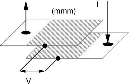
Figure 1: Four terminal set-up for testing DC Josephson-like effect

One way to test the zero voltage drop is through a sample with the geometry described in Fig. 1. The middle region is occupied by the $(mmm)$ state, and the left and the right region by a metallic state (e.g. the $\nu=1/2$ state) in the first and second layer respectively. The metallic state in the R and L region serve as ohmic contacts to the first and second layer in the $(mmm)$ state. One voltage probe is attached to an edge of the $(mmm)$ state in the first layer, and the other attached to the edge on the same side in the second layer (see Fig. 1). As we pass a current from the right region to the left region, the current must tunnel through the barrier between the two layer. According to Ref. [2], if the current is less than a critical value (here we assume a uniform interlayer tunneling), the system is described by a time-independent $\theta$ in (17). From (20), we see that such a static configuration does not induce any voltage between the two layers. In other words, the voltage drop between two probes in the two layers would be zero if the probes are on top of each other (i.e. have the same $x$-$y$ coordinates). However, such probes are hard to make in experiments. Since the interlayer tunneling induces a finite energy gap in the bulk of the sample, the chiral edge state does not have any voltage drop along a single edge. Thus we can place the two probes at different place along the edge, as shown in Fig. 1. The voltage drop between the two voltage probes should be zero. For a larger current beyond a critical value, a non-zero voltage drop will be developed. The striking feature is that the voltage drop is zero even for weak interlayer tunneling. Weak interlayer tunneling only leads to a small critical current.

We would like to make four remarks.
(1) If the second voltage probe is attached to the edge on the other side of the sample from the first voltage probe, a non-zero voltage drop will appear due to the non-zero Hall resistance.
(2) The vanishing of the voltage drop between the two leads is a consequence of the superfluidity , not of the chirality of the edge excitations (i.e. the absence of back propagating modes). To illustrate this point let us replace the $(mmm)$ state in the middle region by a $(mm0)$ state, which does not have any superfluidity (i.e. its $K$-matrix does not have a zero eigenvalue). There is no quantum coherence between the two separate $1/m$ states in the two layers. Now interlayer tunneling is controlled by tunneling between the two edges of the two $1/m$ states. In this case a finite current will produce a finite voltage drop between the two layers and hence between the two voltage probes. If the edges are sharp on the scale of the magnetic length, we have[15] $V\propto I^{1/(2m-1)}$ at zero temperature $T=0$ and $(\frac{dI}{dV})_{V=0}\propto T^{2m-2}$.
(3) In the strong tunneling limit, the $(mmm)$ state crosses over to a single layered $\nu=1/m$ state. The zero voltage drop between the two leads is just the standard result $\rho_{xx}=0$ for fractional quantum Hall states. This correct cross-over behavior from the weak to the strong tunneling limit further confirms the validity of our results.
(4) If the interlayer tunneling is not uniform, the flux trapped between the layers should be pinned to observe the DC Josephson-like effect[19, 20].

Before closing this section, we would like to mention that in a two-terminal measurement as arranged in Fig. 1, the measured two-terminal resistance should be exactly $mh/e^{2}$ for the $(mmm)$ state if the current is smaller than a critical value. Note that the small-current two-terminal resistance is always $mh/e^{2}$ regardless the strength the interlayer tunneling amplitude, despite the tunneling current flows across the interlayer junction. This resembles the zero DC resistance of a Josephson junction between two superconductors at small currents. A small interlayer tunneling only reduces the value of the critical current. For current beyond the critical value, the two-terminal resistance will become very large in the weak tunneling limit.

5 Quantized Hall drag resistance

Recently Kellogg et al[21] has observed a quantized Hall drag resistance in $(111)$ state, as predicted by several groups.[22, 23, 24, 25] Here we would like to show that quantized Hall drag resistance can be easily obtained using the $K$-matrix Chern-Simon effective theory. This allows us to calculate the Hall drag for any Abelian quantum Hall state characterized by $K$.

For simplicity, let us consider a double layer state characterized by a $2\times 2$ $K$-matrix. The effective theory is given by

$$\mathcal{L}_{Hall}=\sum_{I,J}(\frac{K_{IJ}}{4\pi}\varepsilon^{\mu\nu\lambda}a_{\mu}^{I}\partial_{\nu}a_{\lambda}^{J})+\sum_{I}(\frac{1}{2\pi}\varepsilon^{\mu\nu\lambda}a_{\mu}^{I}\partial_{\nu}A_{\lambda}^{I})$$ (22)

where $A^{I}_{\mu}$, $I=1,2$, is the electromagnetic gauge potential in the $I^{th}$ layer. From the equation of motion, we find that the induced current in the two layers, $j^{I}_{\mu}=\frac{1}{2\pi}\varepsilon^{\mu\nu\lambda}\partial_{\nu}a_{\lambda}^{I}$, are given by

$$j^{I}_{i}=\frac{e^{2}}{h}(K^{-1})^{IJ}\varepsilon^{ij}E_{j}^{J}$$ (23)

where $E_{i}^{I}$ is the electric field in the $I^{th}$ layer, and $i,j=x,y$. We can define the Hall drag resistance, $R_{xy,IJ}$, as the coefficiant that determine the Hall voltage in the $I^{th}$ layer induced by the current in the $J^{th}$ layer

$$E_{i}^{I}=R_{xy,IJ}\varepsilon^{ij}j_{i}^{J}$$ (24)

We find $R_{xy,IJ}$ is given by

$$R_{xy,IJ}=\frac{h}{e^{2}}K_{IJ}$$ (25)

The above result applies to any double-layer quantum Hall state characterized by the $2\times 2$ $K$-matrix. It is interesting to see that the $K$-matrix can be directly measured via the Hall drag matrix. For the $(klm)$ state, $K_{11}=k$, and $K_{12}=m$. We have

$$R_{xy,11}=\frac{kh}{e^{2}},\ \ \ \ R_{xy,12}=\frac{mh}{e^{2}}$$ (26)

which is exactly what was observed by Kellogg et al for the $(111)$ state.

6 Summary

The superfluidity/superconductivity in certain quantum Hall state reveals a subtle quantum correlation. Using the $K$-matrix description of the quantum Hall states, we can identify exactly which quantum Hall states have such special correlation. We find that if $K$ has a zero eigenvalue, then the corresponding quantum Hall state may have a spontaneously broken $U(1)$ symmetry and the associated superfluidity/superconductivity. The picture presented in this paper reveal the basic physics behind the superfluidity/superconductivity in quantum Hall states. Our formalism can be applied to more general quantum Hall systems well beyond the double layer system, to multi-layered systems for example. We also proposed a concrete four-terminal test for the DC Josephson-like effect. We hope that the controversy around the superfluidity/superconductivity in the $(mmm)$ state and the DC Josephson-like effect in the interlayer tunneling can be settled by experiments. Also we would like to point out that observing the AC Josephson-like effect (a peak at $f_{J}^{*}$ in the noise spectrum of interlayer tunneling current) will truly reveal the unusual correlation in the $(mmm)$ state.

7 Acknowledgment

We thank Professor H. T. Nieh for his hospitality at the Center for Advanced Study, Tsinghua University, Beijing, China. XGW is supported by NSF Grant No. DMR–01–23156 and by NSF-MRSEC Grant No. DMR–98–08941, and AZ by NSF Grant No. PHY-99-07949.

References

- [1] X.G. Wen and A. Zee, Phys. Rev. Lett. 69 1811 (1992).
- [2] X.G. Wen and A. Zee, Phys. Rev. B47 2265 (1993).
- [3] X.G. Wen and A. Zee, Europhys. Lett. 35 227 (1996).
- [4] X.G. Wen and A. Zee, A Phenomenological Study of Interlayer Tunneling in Double-Layered Quantum Hall Systems, MIT-ITP preprint, http://dao.mit.edu/~wen, (1994).
- [5] I. B. Spielman, J. P. Eisenstein, L. N. Pfeiffer, K. W. West, Phys. Rev. Lett. 84 5808 (2000); I. B. Spielman, J. P. Eisenstein, L. N. Pfeiffer, K. W. West, cond-mat/0012094.
- [6] H.A. Fertig, Phys. Rev. B40 1087 (1989).
- [7] A.H. MacDonald, P.M. Platzman, and G.S. Boebinger, Phys. Rev. Lett. 65, 775 (1990).
- [8] L. Brey, Phys. Rev. Lett. 65, 903 (1990).
- [9] K. Yang, K. Moon, L. Zheng, A. MacDonald, S. Girvin, D. Yoshioka, and S.-C. Zhang, Phys. Rev. Lett. 73 732 (1994).
- [10] A. H. MacDonald and Shou-Cheng Zhang, Phys. Rev. B49 17208 (1994).
- [11] Y. N. Joglekar and A. H. MacDonald, cond-mat/0103454.
- [12] X. G. Wen, Advances in Physics 44 405 (1995).
- [13] A. Zee, “Quantum Hall Fluids”, in Field Theory, Topology and Condensed Matter Physics, ed. by H.B. Geyer, (Springer-Verlag, 1994).
- [14] F. Wilczek and A. Zee, Phys. Rev. Lett. 51 2250 (1983).
- [15] X.G. Wen, Int. J. Mod. Phys., B6 1711 (1992).
- [16] R. P. Feynman, Statistical Mechanics, (Perseus, 1990).
- [17] X.G. Wen and A. Zee, Nucl. Phys. (Suppl.) B15 135 (1990); B. Blok and X.G. Wen, Phys. Rev. B42 8133 (1990); Phys. Rev. B42 8145 (1990); N. Read, Phys. Rev. Lett. 65 1502 (1990); J. Fröhlich and A. Zee, Nucl. Phys. B364 517 (1991).
- [18] X.G. Wen and A. Zee, Phys. Rev. B46 2290 (1992). X.G. Wen and A. Zee, Phys. Rev. B58 15717 (1998).
- [19] L. Balents and L. Radzihovsky, Phys. Rev. Lett. 86 1825 (2001).
- [20] M. M. Fogler, F. Wilczek, Phys. Rev. Lett. 86 1833 (2001).
- [21] M. Kellogg, et al, cond-mat/0108403.
- [22] K. Moon, et al, Phys. Rev. B, 51, 5138 (1995)
- [23] J.-M., Duan, Europhys. Lett., 29, 489 (1995)
- [24] K. Yang, et al, Phys. Rev. B, 58, R4246 (1998)
- [25] Y.B. Kim, et al, cond-mat/0011459.