Dynamics of quantum Hall stripes in double-quantum-well systems

Abstract

The collective modes of stripes in double layer quantum Hall systems are computed using the time-dependent Hartree-Fock approximation. It is found that, when the system possesses spontaneous interlayer coherence, there are two gapless modes, one a phonon associated with broken translational invariance, the other a pseudospin-wave associated with a broken $U(1)$ symmetry. For large layer separations the modes disperse weakly for wavevectors perpendicular to the stripe orientation, indicating the system becomes akin to an array of weakly coupled one-dimensional $XY$ systems. At higher wavevectors the collective modes develop a roton minimum associated with a transition out of the coherent state with further increasing layer separation. A spin wave model of the system is developed, and it is shown that the collective modes may be described as those of a system with helimagnetic ordering.

PACS: 73.20.Mf,73.21.Fg,71.10.Hf

I Introduction and Summary of Results

Quantum Hall systems are by now well-known to support a broad range of condensed matter phenomena[1]. These include localization physics, electron solidification (Wigner crystals), chiral Luttinger liquids at quantum Hall edges, and Fermi liquid behavior. Recently added to this list is highly anisotropic transport in moderate magnetic fields, in which electrons populate several Landau levels[2]. Such behavior was anticipated by mean-field studies predicting unidirectional charge density wave (CDW) ground states for electrons in high Landau levels[3, 4]. While more careful studies[5] demonstrate that within Hartree-Fock theory such ground states are unstable to the formation of “modulated” stripe states which are essentially highly anisotropic two-dimensional Wigner crystals (“stripe crystals” [6]), quantum fluctuations may restore the translational symmetry along the stripes[7, 8, 9, 10]. It has been noted that the CDW state has the symmetry of a two-dimensional smectic[6], and this analogy with liquid crystals has been exploited to yield a number of useful results[11].

A seemingly unrelated set of physical phenomena occurs in double quantum well systems (DQWS) in the quantum Hall regime. For large magnetic fields, these systems support spontaneous interlayer coherence[12], and exhibit an associated Goldstone mode[13, 14]. A precursor of the Josephson tunneling[15, 16] may have been observed[17] in these systems, contributing to recent excitement about them.

When immersed in more moderate magnetic fields, such that several Landau levels are occupied, it becomes evident that the physics of stripes and interlayer coherence are simultaneously relevant in the bilayer system. This situation was recently explored[18]. For a system in which each layer is half-filled in the $Nth$ Landau level, with some simplifying assumptions (lower Landau levels filled and inert, Landau level mixing negligible, and Zeeman coupling large enough that spins are polarized) it was found that: (1) For small enough layer separation, and any value of $N$, an interlayer coherent state of uniform density is formed. (2) Above a critical layer separation $d_{c}(N)$, a unidirectional density modulation sets in such that the electron density oscillates between the layers as a function of position [19]. This state is simultaneously interlayer coherent and smectic in spatial symmetry. With increasing $d$, the regions of coherence become relatively narrow in one direction, forming “linear coherent regions” (LCR’s). (3) For negligibly weak interlayer tunneling, the coherence is spontaneous and a corresponding Goldstone mode should be present in the excitation spectrum. When the LCR’s are sufficiently narrow compared to their separation (which occurs at large $d$ and/or large $N$), the system may be thought of as an array of coupled one-dimensional XY models. Different possible quantum-disordered states may exist[18, 20], which in principle can be distinguished by tunneling experiments.

In order to predict which, if any, of these quantum disorderings might occur, it is necessary to understand the low-energy collective modes in some detail, and to create a model that captures them which is sufficiently simple to be susceptible to further analysis[8]. This motivates our present study. Beyond its use in specifying a low-energy theory, the collective modes are interesting on their own, as they are sometimes detectible in electromagnetic absorption[21] or Raman scattering[22] experiments, and allow one to learn about which states are realized in real samples.

In what follows, we compute the collective mode spectrum of the electrons in a DQWS, in a perpendicular magnetic field, in which several Landau levels are occupied, using the time-dependent Hartree-Fock approximation (TDHFA) [23]. Counting both the spin and layer index degrees of freedom, the situations we consider involve $4N$ filled Landau levels, which are taken to be inert (as appropriate for large cyclotron energy $\hbar\omega_{c}$, where $\omega_{c}=eB/m^{*}c$, $B$ is the magnetic field, and $m^{*}$ the effective mass of electrons in the quantum wells, and large Zeeman coupling.) For simplicity we ignore finite thickness of the wells. In addition to the $4N$ filled levels, there is a level, with Landau index $N$, which contains precisely enough electrons so that the total filling factor $\nu$, defined as the number of electrons per magnetic flux quantum passing through the plane, is $4N+1$. The system considered has no interlayer bias, so that the highest level in each layer will be half-filled on average.

As discussed above, if the individual layers are isolated, this is precisely the situation in which one expects stripes to form. For finite layer separations, it is clear that the ground state will have the electron-rich regions in one layer align directly above the hole-rich regions in the other. Furthermore, for a range of layer separations, the stripe edges hybridize between the layers so that the electron occupation continuously shifts between the layers as a function of position[18]. An example of such a ground state is illustrated in Fig. 2. To understand this state and its collective modes it is convenient to adopt a pseudospin representation, in which an electron pseudospin is “up” when occupying one layer, and “down” when occupying the other. In this language, the stripe ground state involves a unidirectional spatial tumbling of the spin, and may be thought of as having helimagnetic ordering[24]. As the separation increases, the electron density tends to reside more sharply in one well or the other, and the transition regions between layers become narrower[18].

In the absence of interlayer tunneling, the pseudospin density may tumble from $+\hat{z}$ to $-\hat{z}$ by passing through the $\hat{x}$ direction, the $\hat{y}$ direction, or any direction in between. Thus, each of the transition regions – the LCR’s mentioned above – supports an $XY$ degree of freedom, which is spontaneously broken in the ground state. In addition, this state obviously has broken translational symmetry.

Because of the two broken symmetries, there are two gapless excitations above the stripe ground state. One is associated with the broken $XY$ symmetry – alternatively thought of as a phase coherence between the wells[12, 13] – which disperses linearly with wavevector. The other is a phonon-like mode which disperses quadratically for wavevectors parallel to the stripes, and linearly perpendicular to them. This is analogous to what is seen in incommensurate helimagnets[24].

A typical dispersion relation for the $XY$ mode is displayed in Fig. 5 for several values of $d/\ell$, where $\ell=\sqrt{\hbar c/eB}$ is the magnetic length. As may be seen, the linear mode tends to disperse more strongly along the stripes than perpendicular to them, and in the limit of large $d$, the latter dispersion may become quite weak. This may be understood in terms of the exchange coupling among LCR’s, which vanishes as they become arbitrarily narrow[18]. It is possible that quantum fluctuations can effectively wipe out the inter-LCR exchange coupling, leading to a state analogous to a “sliding $XY$ model”[18, 25].

Several other features appear in the collective mode spectrum. As is typical of such calculations, a number of higher energy modes are present, one of which may be interpreted as a gapped “out-of-phase” phonon mode, in which the stripes in different layers oscillate against one another. In Fig. 5, we see that this mode becomes degenerate with the $XY$ mode in its dispersion relation along the stripe direction and develops a roton minimum which touches zero at a critical separation $d_{M}$, signaling an instability in which modulations form along the stripes. The instability, however, is first-order in nature since the modulation amplitude changes discontinuously at the transition[18]. It is a surprising feature of our results that a collective mode appears to go soft so close to this transition, and this behavior in principle allows a detection of the transition by inelastic light scattering. Whether such a bilayer stripe crystal is stable with respect to quantum fluctuations analogous to those being discussed in the single layer case[7, 8, 9, 10] is at present unclear.

This article is organized as follows. In Section II we sketch the Hartree-Fock and TDHFA formalism, providing some details about its application to the two-layer stripe system. Section III contains a more detailed description of our results, and Section IV shows how the low-energy spectrum may be understood in the pseudospin language. We conclude with a summary and discussion in Section V.

II Hartree-Fock description of the CDW ground state

We consider an unbiaised symmetric DQWS in a perpendicular magnetic field ${\bf B}=B{\bf z}$ at total filling factor $\nu=4N+\nu_{0}$ where $N=0,1,2,...$ is the Landau level index and $\nu_{0}$ is the filling factor of the partially filled level. Each Landau level has two spin states and two layer states specified by the index $j=R,L$. The layer states hybridize into symmetric (S) and antisymmetric (AS) states in the presence of tunneling. We assume the magnetic field to be strong enough so that the lower $4N$ levels are completely filled with electrons and can be considered as inert. The Zeeman energy is assumed to be much larger than the S-AS gap and so there is no spin texture in the ground state. The electron gas is completely spin polarised and only the layer degree of freedom need be considered. In the ground state, the electronic charge is equally distributed between the two wells.

In the Landau gauge where the vector potential ${\bf A}=(0,Bx,0)$, the electron wavefunctions are given by

$$\psi_{N,X,j}({\bf r})=\frac{1}{\sqrt{L_{y}}}e^{-iXy/\ell^{2}}\varphi_{N}\left(x-X\right)\chi_{j}(z),$$ (1)

where $N$ and $X$ are the Landau level and guiding center indices and $\chi_{j}(z)$ is the envelope wave function of the lowest-energy electric subband centered on the right or left well. $\varphi_{N}\left(x\right)$ is an eigenfunction of the one-dimensional harmonic oscillator. Because the fully occupied Landau levels are considered as inert, we need only consider the partially filled Landau level. We can then drop the Landau level index from now on.

To describe the various charge density wave (CDW) ground states, we define the operator

$$\rho_{i,j}({\bf q})=\frac{1}{N_{\varphi}}\sum_{X}e^{-iq_{x}X+iq_{x}q_{y}\ell^{2}/2}\ c_{i,X}^{\dagger}c_{j,X-q_{y}\ell^{2}},$$ (2)

where $i,j=R,L$ and $N_{\varphi}$ is the Landau level degeneracy. In the ground state, $\left\langle\rho_{i,j}({\bf q})\right\rangle\neq 0$ where ${\bf q}$ is a reciprocal lattice vector of the CDW. By definition $\left\langle\rho_{R,R}({\bf q}=0)\right\rangle=\left\langle\rho_{L,L}({\bf q}=0)\right\rangle=\nu_{0}/2$. In the Hartree-Fock approximation (HFA), the ground-state energy per electron in units of $e^{2}/\kappa\ell$ in the partially filled level can be written in term of these operators as

$$E_{HF} = -\frac{2}{\nu_{0}}t\mathop{\rm Re}\left[\left\langle\rho_{R,L}\left({\bf q}=0\right)\right\rangle\right]$$ (6)

$$+\frac{1}{2\nu_{0}}\sum_{{\bf q}}\left[H\left({\bf q}\right)-X\left({\bf q}\right)\right]\left[\left|\left\langle\rho_{R,R}\left({\bf q}\right)\right\rangle\right|^{2}+\left|\left\langle\rho_{L,L}\left({\bf q}\right)\right\rangle\right|^{2}\right]$$

$$+\frac{1}{\nu_{0}}\sum_{{\bf q}}\widetilde{H}\left({\bf q}\right)\left\langle\rho_{R,R}\left({\bf q}\right)\right\rangle\left\langle\rho_{L,L}\left(-{\bf q}\right)\right\rangle$$

$$-\frac{1}{\nu_{0}}\sum_{{\bf q}}\widetilde{X}\left({\bf q}\right)\left\langle\rho_{R,L}\left(-{\bf q}\right)\right\rangle\left\langle\rho_{L,R}\left({\bf q}\right)\right\rangle.$$

In this equation, $t$ is the tunneling energy in units of $e^{2}/\kappa\ell$, and $H\left({\bf q}\right),X\left({\bf q}\right)$ are the Hartree and Fock intra-well interactions while $\widetilde{H}\left({\bf q}\right)$ and $\widetilde{X}\left({\bf q}\right)$ are the Hartree and Fock inter-well interactions. For very narrow wells where $\chi_{j}(z)$ are highly localized, these interactions are given by

$$\begin{array}[]{rll}H({\bf q})&=&\left(\frac{1}{q\ell}\right)\left[L_{N}^{0}\left(q^{2}\ell^{2}/2\right)\right]^{2}e^{-q^{2}\ell^{2}/2},\\ \widetilde{H}({\bf q})&=&\left(\frac{1}{q\ell}\right)\left[L_{N}^{0}\left(q^{2}\ell^{2}/2\right)\right]^{2}e^{-q^{2}\ell^{2}/2}e^{-qd},\\ X({\bf q})&=&\int_{0}^{\infty}dyJ_{0}(yq\ell)e^{-y^{2}/2}\left[L_{N}^{0}\left(y^{2}/2\right)\right]^{2},\\ \widetilde{X}({\bf q})&=&\int_{0}^{\infty}dyJ_{0}(yq\ell)e^{-y^{2}/2}e^{-yd/\ell}\left[L_{N}^{0}\left(y^{2}/2\right)\right]^{2},\end{array}$$ (7)

where $d$ is the center-to-center separation between the wells and $L_{N}^{0}\left(x\right)$ are generalized Laguerre polynomials. Because of the neutralizing positive backgrounds of ionized donors on both sides of the DQWS, we have $H\left(0\right)=\widetilde{H}\left(0\right)=0$ in $E_{HF}$.

The order parameters $\left\{\left\langle\rho_{i,j}\left({\bf q}\right)\right\rangle\right\}$ are computed by solving the HF equations of motion for the single-particle Green’s function

$$G_{i,j}\left(X,X^{\prime},\tau\right)=-\left\langle Tc_{i,X}\left(\tau\right)c_{j,X^{\prime}}^{\dagger}\left(0\right)\right\rangle$$ (8)

whose Fourier transform we define as

$$G_{i,j}\left({\bf q,}\tau\right)=\frac{1}{N_{\phi}}\sum_{X,X^{\prime}}e^{-\frac{i}{2}q_{x}\left(X+X^{\prime}\right)}\delta_{X,X^{\prime}-q_{y}l^{2}}G_{i,j}\left(X,X^{\prime},\tau\right),$$ (9)

so that $G_{i,j}\left({\bf q,}\tau=0^{-}\right)=\left\langle\rho_{j,i}\left({\bf q}\right)\right\rangle.$

In the HFA, these equations of motion are given by

$$\sum_{{\bf q}^{\prime\prime}}\left(\begin{array}[]{cc}\left(i\hslash\omega_{n}+\mu\right)\delta_{{\bf q},{\bf q}^{\prime\prime}}-U_{R,R}\left({\bf q,q}^{\prime\prime}\right)&t\delta_{{\bf q},{\bf q}^{\prime\prime}}-U_{R,L}\left({\bf q,q}^{\prime\prime}\right)\\ t\delta_{{\bf q},{\bf q}^{\prime\prime}}-U_{L,R}\left({\bf q,q}^{\prime\prime}\right)&\left(i\hslash\omega_{n}+\mu\right)\delta_{{\bf q},{\bf q}^{\prime\prime}}-U_{L,L}\left({\bf q,q}^{\prime\prime}\right)\end{array}\right)$$ (12)

$$\left(\begin{array}[]{cc}G_{R,R}\left({\bf q}^{\prime\prime},\omega_{n}\right)&G_{R,L}\left({\bf q}^{\prime\prime},\omega_{n}\right)\\ G_{L,R}\left({\bf q}^{\prime\prime},\omega_{n}\right)&G_{L,L}\left({\bf q}^{\prime\prime},\omega_{n}\right)\end{array}\right)=\left(\begin{array}[]{cc}\hslash\delta_{{\bf q},0}&0\\ 0&\hslash\delta_{{\bf q},0}\end{array}\right)$$ (17)

where $\mu$ is the chemical potential. The effective potentials $U_{i,j}$ (in units of $e^{2}/\kappa\ell$) are defined by

$$U_{R,R}\left({\bf q,q}^{\prime}\right)=\left[H\left({\bf q-q}^{\prime}\right)-X\left({\bf q-q}^{\prime}\right)\right]\left\langle\rho_{R,R}\left({\bf q-q}^{\prime}\right)\right\rangle\gamma_{{\bf q},{\bf q}^{\prime}}+\widetilde{H}\left({\bf q-q}^{\prime}\right)\left\langle\rho_{L,L}\left({\bf q-q}^{\prime}\right)\right\rangle\gamma_{{\bf q},{\bf q}^{\prime}},$$ (18)

$$U_{L,L}\left({\bf q,q}^{\prime}\right)=\left[H\left({\bf q}-{\bf q}^{\prime}\right)-X\left({\bf q}-{\bf q}^{\prime}\right)\right]\left\langle\rho_{L,L}\left({\bf q-q}^{\prime}\right)\right\rangle\gamma_{{\bf q},{\bf q}^{\prime}}+\widetilde{H}\left({\bf q}-{\bf q}^{\prime}\right)\left\langle\rho_{R,R}\left({\bf q-q}^{\prime}\right)\right\rangle\gamma_{{\bf q},{\bf q}^{\prime}},$$ (19)

$$U_{R,L}\left({\bf q,q}^{\prime}\right)=-\widetilde{X}\left({\bf q}-{\bf q}^{\prime}\right)\left\langle\rho_{L,R}\left({\bf q-q}^{\prime}\right)\right\rangle\gamma_{{\bf q},{\bf q}^{\prime}},$$ (20)

$$U_{L,R}\left({\bf q,q}^{\prime}\right)=-\widetilde{X}\left({\bf q}-{\bf q}^{\prime}\right)\left\langle\rho_{R,L}\left({\bf q-q}^{\prime}\right)\right\rangle\gamma_{{\bf q},{\bf q}^{\prime}},$$ (21)

where $\gamma_{{\bf q},{\bf q}^{\prime}}=e^{-i{\bf q}\times{\bf q}^{\prime}l_{\bot}^{2}/2}$. The procedure to solve for the $\left\langle\rho_{i,j}\left({\bf q}\right)\right\rangle^{\prime}s$ is described in detail in Ref.[23].

It is instructive at this point to describe the electron state in a DQWS by using a pseudospin language where states $R$ and $L$ are mapped to up and down spin states. For this, we define the pseudospin operators

$$\rho\left({\bf q}\right) = \frac{1}{2}\left[\rho_{R,R}\left({\bf q}\right)+\rho_{L,L}\left({\bf q}\right)\right],$$ (22)

$$\rho_{x}\left({\bf q}\right) = \frac{1}{2}\left[\rho_{R,L}\left({\bf q}\right)+\rho_{L,R}\left({\bf q}\right)\right],$$ (23)

$$\rho_{y}\left({\bf q}\right) = \frac{1}{2i}\left[\rho_{R,L}\left({\bf q}\right)-\rho_{L,R}\left({\bf q}\right)\right],$$ (24)

$$\rho_{z}\left({\bf q}\right) = \frac{1}{2}\left[\rho_{R,R}\left({\bf q}\right)-\rho_{L,L}\left({\bf q}\right)\right],$$ (25)

$${\bf\rho}_{\bot}\left({\bf q}\right) = \rho_{x}\left({\bf q}\right)\widehat{{\bf x}}+\rho_{y}\left({\bf q}\right)\widehat{{\bf y}}.$$ (26)

These operators act in the restricted Hilbert space of the partially filled Landau level. To get a real space representation of the ordered states, we take the Fourier transform

$$\left\langle\rho_{i,j}\left({\bf r}\right)\right\rangle=\sum_{{\bf q}}\left\langle\rho_{i,j}\left({\bf q}\right)\right\rangle e^{i{\bf q}\cdot{\bf r}}.$$ (27)

A local filling factor in each well can then be defined as

$$\nu_{i}\left({\bf r}\right)=\left\langle\rho_{i,i}\left({\bf r}\right)\right\rangle.$$ (28)

For unidirectional modulations, the quantity $\nu_{i}\left({\bf r}\right)$ will take values between $0$ and $1.$ Similarly, a Fourier transform of the order parameters defined in Eq. (22) will define the total density $\left\langle\rho\left({\bf r}\right)\right\rangle$ and spin density $\left\langle\rho_{\mu}\left({\bf r}\right)\right\rangle$. Note that these densities are related to the density of orbit centers and not to the real density of electrons. For instance, when Landau mixing is neglected, the real “densities” $n_{i,j}\left({\bf q}\right)$ are given by

$$n_{i,j}\left({\bf q}\right)=N_{\phi}F_{N}\left({\bf q}\right)\rho_{i,j}\left({\bf q}\right)$$ (29)

where $F_{N}\left({\bf q}\right)$ is a form factor appropriate to Landau level $N$ given by

$$F_{N}\left({\bf q}\right)=\exp\left(\frac{-q^{2}l^{2}}{4}\right)L_{N}^{0}\left(\frac{q^{2}l^{2}}{2}\right).$$ (30)

In the pseudospin language, the HF energy can be rewritten as

$$E_{HF} = -\frac{2}{\nu_{0}}t\mathop{\rm Re}\left[\left\langle\rho_{x}\left(0\right)\right\rangle\right]$$ (34)

$$+\frac{1}{\nu_{0}}\sum_{{\bf q}}\Upsilon\left({\bf q}\right)\left\langle\rho\left(-{\bf q}\right)\right\rangle\left\langle\rho\left({\bf q}\right)\right\rangle$$

$$+\frac{1}{\nu_{0}}\sum_{{\bf q}}J_{z}\left({\bf q}\right)\left\langle\rho_{z}\left(-{\bf q}\right)\right\rangle\left\langle\rho_{z}\left({\bf q}\right)\right\rangle$$

$$+\frac{1}{\nu_{0}}\sum_{{\bf q}}J_{\bot}\left({\bf q}\right)\left\langle{\bf\rho}_{\bot}\left(-{\bf q}\right)\right\rangle\cdot\left\langle{\bf\rho}_{\bot}\left({\bf q}\right)\right\rangle.$$

where the effective interactions are defined by

$$\Upsilon\left({\bf q}\right) = H\left({\bf q}\right)+\widetilde{H}\left({\bf q}\right)-X\left({\bf q}\right),$$ (35)

$$J_{z}\left({\bf q}\right) = H\left({\bf q}\right)-\widetilde{H}\left({\bf q}\right)-X\left({\bf q}\right),$$ (36)

$$J_{\bot}\left({\bf q}\right) = -\widetilde{X}\left({\bf q}\right).$$ (37)

We derive the dispersion relations of the collective excitations of the CDW states in the DQWS by tracking the poles of the retarded density and pseudospin response functions. These are obtained by analytical continuation of the two-particle Matsubara Green’s functions

$$\chi_{i,j,k,l}\left({\bf q,q}^{\prime};\tau\right)=-N_{\phi}\left\langle T\rho_{i,j}\left({\bf q,}\tau\right)\rho_{k,l}\left(-{\bf q}^{\prime},0\right)\right\rangle+N_{\phi}\left\langle\rho_{i,j}\left({\bf q}\right)\right\rangle\left\langle\rho_{k,l}\left(-{\bf q}^{\prime}\right)\right\rangle$$ (38)

which we compute in the generalized random phase approximation (GRPA). The procedure is explained in details in Refs.[5, 23]. It is convenient to work in the pseudospin language where we can define the matrix

$$\chi=\left(\begin{array}[]{cccc}\chi_{\rho,\rho}&\chi_{\rho,x}&\chi_{\rho,y}&\chi_{\rho,z}\\ \chi_{x,\rho}&\chi_{x,x}&\chi_{x,y}&\chi_{x,z}\\ \chi_{y,\rho}&\chi_{y,x}&\chi_{y,y}&\chi_{y,z}\\ \chi_{z,\rho}&\chi_{z,x}&\chi_{z,y}&\chi_{z,z}\end{array}\right).$$ (39)

These pseudospin Green’s functions are related to the original Green’s functions of eq. (38) by the transformation

$${\chi}^{\nu,\mu}=\frac{1}{4}\sigma_{i,j}^{\nu}\chi_{i,j,k,l}\sigma_{k,l}^{\mu},$$ (40)

where $\nu,\mu=\rho,x,y,z.$ $\sigma_{i,j}^{\nu=x,y,z}$ are Pauli matrices and $\sigma^{\rho}=\left(\begin{array}[]{cc}1&0\\ 0&1\end{array}\right).$

The summation of the bubbles and ladder diagrams of the GRPA can be expressed as an equation of motion for $\chi$ of the form

$$\left(\omega+i\delta\right)\chi\left({\bf q},{\bf q}^{\prime},\omega\right)-\sum_{{\bf q}^{\prime\prime}}F\left({\bf q},{\bf q}^{\prime\prime}\right)\chi\left({\bf q}^{\prime\prime},{\bf q}^{\prime},\omega\right)=D\left({\bf q},{\bf q}^{\prime}\right).$$ (41)

Here $F$ and $D$ may be written schematically as

$$F=-2i\left(\begin{array}[]{cccc}\left\langle\rho\right\rangle\sin a\left[\Upsilon-\Upsilon^{\prime}\right]&\left\langle\rho_{x}\right\rangle\sin a\left[J_{\bot}-J_{\bot}^{\prime}\right]&\left\langle\rho_{y}\right\rangle\sin a\left[J_{\bot}-J_{\bot}^{\prime}\right]&\left\langle\rho_{z}\right\rangle\sin a\left[J_{z}-J_{z}^{\prime}\right]\\ \left\langle\rho_{x}\right\rangle\sin a\left[J_{\bot}-\Upsilon^{\prime}\right]&\left\langle\rho\right\rangle\sin a\left[\Upsilon-J_{\bot}^{\prime}\right]&\left\langle\rho_{z}\right\rangle\cos a\left[J_{z}-J_{\bot}^{\prime}\right]&-\left\langle\rho_{y}\right\rangle\cos a\left[J_{\bot}-J_{z}^{\prime}\right]\\ \left\langle\rho_{y}\right\rangle\sin a\left[J_{\bot}-\Upsilon^{\prime}\right]&-\left\langle\rho_{z}\right\rangle\cos a\left[J_{z}-J_{\bot}^{\prime}\right]&\left\langle\rho\right\rangle\sin a\left[\Upsilon-J_{\bot}^{\prime}\right]&t+\left\langle\rho_{x}\right\rangle\cos a\left[J_{\bot}-J_{z}^{\prime}\right]\\ \left\langle\rho_{z}\right\rangle\sin a\left[J_{z}-\Upsilon^{\prime}\right]&\left\langle\rho_{y}\right\rangle\cos a\left[J_{\bot}-J_{\bot}^{\prime}\right]&t-\left\langle\rho_{x}\right\rangle\cos a\left[J_{\bot}-J_{\bot}^{\prime}\right]&\left\langle\rho\right\rangle\sin a\left[\Upsilon-J_{z}^{\prime}\right]\end{array}\right),$$ (42)

and

$$D=\left(\begin{array}[]{cccc}i\left\langle\rho\right\rangle\left(\sin a\right)&i\left\langle\rho_{x}\right\rangle\left(\sin a\right)&i\left\langle\rho_{y}\right\rangle\left(\sin a\right)&i\left\langle\rho_{z}\right\rangle\left(\sin a\right)\\ i\left\langle\rho_{x}\right\rangle\left(\sin a\right)&i\left\langle\rho\right\rangle\left(\sin a\right)&i\left\langle\rho_{z}\right\rangle\cos a&-i\left\langle\rho_{y}\right\rangle\left(\cos a\right)\\ i\left\langle\rho_{y}\right\rangle\left(\sin a\right)&-i\left\langle\rho_{z}\right\rangle\cos a&i\left\langle\rho\right\rangle\left(\sin a\right)&i\left\langle\rho_{x}\right\rangle\left(\cos a\right)\\ i\left\langle\rho_{z}\right\rangle\left(\sin a\right)&i\left\langle\rho_{y}\right\rangle\left(\cos a\right)&-i\left\langle\rho_{x}\right\rangle\left(\cos a\right)&i\left\langle\rho\right\rangle\left(\sin a\right)\end{array}\right).$$ (43)

These matrices contain wavevector dependence that is not shown. For example, in the $F$ matrix, the first entry is explicitly given by

$$-2i\left\langle\rho\right\rangle\sin a\left[\Upsilon-\Upsilon^{\prime}\right]\rightarrow-2i\left\langle\rho\left({\bf q}-{\bf q}^{\prime\prime}\right)\right\rangle\sin\left[\frac{{\bf q}\times{\bf q}^{\prime\prime}l_{\bot}^{2}}{2}\right]\left[\Upsilon\left({\bf q}-{\bf q}^{\prime\prime}\right)-\Upsilon\left({\bf q}^{\prime\prime}\right)\right].$$ (44)

The other terms in the matrix, as well as those in the matrix $D$, have analogous definitions. Finally, for the tunneling term in $F_{34}$ and $F_{43}$ is diagonal in the wavevector index i.e. $t\rightarrow$ $t\delta_{{\bf q},{\bf q}^{\prime\prime}}.$ Eq. (41) may be solved by diagonalizing $F$ [23], and the collective mode frequencies found from its eigenvalues. From the eigenvectors of the $F$ matrix, it is also possible to extract the motion of the guiding-center densities and of the pseudospin in a given mode.

It is interesting to note that for $\left\langle\rho_{x,y}\right\rangle=0$ and $t=0$, the forms of $F$ and $D$ indicate that in the equations of motion $\chi_{\rho,\rho},~{}\chi_{\rho,z},~{}\chi_{z,\rho},~{}\chi_{z,z}$ completely decouple from $\chi_{xx},~{}\chi_{xy},~{}\chi_{yx},~{}\chi_{yy}$. This indicates that distortions of the stripes involving motion of charge either within the layers or between them is completely decoupled from any “in-plane” $XY$ motion of the pseudospins; i.e., phonon modes and spin-wave modes will create poles in different, distinct response functions. The presence of coherence – a non-vanishing $\left\langle\rho_{x}\right\rangle$ or $\left\langle\rho_{y}\right\rangle$ – mixes these motions, so that poles from all the collective modes appear in all the response functions. This phenomenon is closely related to “spin-charge coupling” that is generically present in multicomponent quantum Hall systems [1], and has important consequences for the charged excitations in this system [18]. For the collective modes, we will see below that the low-energy interlayer charge degrees of freedom (distortions that change $\rho_{z}$) are in a sense conjugate to the in-plane degrees of freedom ($\rho_{x,y}$), and distortions of both are involved in any given collective mode.

III Numerical results

In Ref. [18] the energies of several ordered ground states at $\nu_{0}=1$ were computed in the HFA. The states considered there were a uniform coherent state (UCS), a unidirectional coherent charge density wave (UCCDW), a modulated unidirectional charge density wave (MUCDW) and a coherent Wigner crystal (CWC) with a square lattice. We refer the reader to Ref. [18] for more detailed discussions of these states. For $N>0$, it was found that the ground state of the electron gas evolves from the UCS for $d<d_{c}\left(N\right)$ to the UCCDW at larger values of $d$ and finally to the MUCDW as the separation between the wells increases. At large $d$, the Wigner crystal state is only lowest in energy for Landau level $N=0$. (There is however a small region of $d$ for $d>d_{c}$ in $N=0$ for which the UCCDW is lowest in energy (see Ref. [18])). For all ordered states, the lowest energy is obtained when the density pattern in both wells are shifted with respect to one another. Moreover, coherent states (states with non-zero value of $\left\langle\rho_{R,L}\left({\bf q}\right)\right\rangle$), when they exist, have lower energy than their incoherent counterparts. For the MUCDW it was impossible to find a coherent version in the region where it has lower energy than the UCCDW. An interesting result of the HF calculation is that the local coherence $\left\langle\rho_{R,L}\left({\bf r}\right)\right\rangle$ is maximal when the charge density is equally shared by both wells. For the UCCDW, this occurs along channels called linear coherent regions (LCR). As the separation between the wells increases, the width of the LCR’s becomes very small. Figs. 1-3 summarizes the HF results for level $N=2$. Fig. 1 shows the energy of the four states defined above as a function of $d$ in Landau level $N=2$ and in the absence of tunneling. (We remark that all results presented in the present paper are for $\nu_{0}=1.$ Also, in the absence of tunneling, the phase of $\left\langle\rho_{R,L}\left({\bf r}\right)\right\rangle$ is arbitrarily choosen so that all spins point in the $\widehat{{\bf x}}$ direction in the ground state). As a measure of the coherence of a given state, we use $\left\langle\rho_{R,L}\left(0\right)\right\rangle.$ This quantity takes its maximal value $1/2$ (at $\nu_{0}=1$) in the UCS. In Fig. 1, the coherence decreases slowly for the UCCDW but very rapidly for the CWC and is essentially zero in the MUCDW.

In Landau level $N=2$, the UCS is lower in energy for $d/\ell<0.7$ at which point it evolves continuously into the UCCDW. At $d/\ell\simeq 1.6$, there is a first order transition into the MUCDW. Fig. 2 shows the guiding- center density in the right and left wells as defined in Eq. (28) and the pseudospin pattern (Eq. (22)) for the UCCDW at $d/\ell=0.7$ and $d/\ell=2.0$. The formation of the LCR’s is clearly visible in this figure. At large $d$, the coherence is very small (see Fig. 1) and the guiding-center densities approach the stripe pattern appropriate to decoupled layers with filling factor $1/2$. For completeness, we also show in Fig. 3 the evolution of band structure[18] $E\left(X\right)$ and of the density of states in the UCCDW at $N=2$ and for $t=0$.

We now consider the collective excitations of the UCS and UCCDW. The dispersion is obtained by solving Eq. (41) for the suceptibility $\chi$. In the UCS, we can easily solve this equation to get the response functions

$$\chi=\allowbreak\left(\begin{array}[]{cccc}0&0&0&0\\ 0&0&0&0\\ 0&0&2\frac{a}{\omega^{2}-4ab}\alpha&i\frac{\omega}{\omega^{2}-4ab}\alpha\\ 0&0&-i\frac{\omega}{\omega^{2}-4ab}a&2\frac{b}{\omega^{2}-4ab}\alpha\end{array}\right),$$ (45)

where

$$\alpha\equiv\left\langle\rho_{x}\left(0\right)\right\rangle,$$ (46)

and

$$a\left({\bf q}\right) = t-\left\langle\rho_{x}\left(0\right)\right\rangle\left[J_{\bot}\left(0\right)-J_{z}\left({\bf q}\right)\right],$$ (47)

$$b\left({\bf q}\right) = t-\left\langle\rho_{x}\left(0\right)\right\rangle\left[J_{\bot}\left(0\right)-J_{\bot}\left({\bf q}\right)\right].$$ (48)

The dispersion relation of the collective mode of the UCS is given by

$$\omega=2\sqrt{a\left({\bf q}\right)b\left({\bf q}\right)}.$$ (49)

This mode is a Goldstone mode (at $t=0$) associated with the broken $XY$ symmetry of the UCS. For small wavevectors, it disperses linearly in $q$ for $t=0$ and $d\neq 0$. This coherence mode represents an elliptical motion of the pseudospins around the $x$ axis. The pseudospin motion becomes more and more confined to the $x-y$ plane as $q$ decreases. For level $N=2$ and in the absence of tunneling, the dispersion relation of this mode softens at interlayer separation $d/\ell\approx 0.64$. This softening occurs at a finite value $q\ell=0.92$ of the wavevector signaling the onset of the formation of the UCCDW state with a wavelength (separation between stripes in a given layer) of approximately $\lambda/\ell=2\pi/0.92.$

For our choice of phase, the pseudospins in the UCCDW rotate in the $x-z$ plane. This implies that $\left\langle\rho_{y}\left({\bf q}\right)\right\rangle=0.$ Moreover, in this shifted state, there is no modulation of the total density, so that $\left\langle\rho\left({\bf q}\right)\right\rangle=0$ as well. The $F$ and $D$ matrix introduced in Eqs. (42) and (43) then simplify to

$$F=-2i\left(\begin{array}[]{cccc}0&\left\langle\rho_{x}\right\rangle\sin a\left[J_{\bot}-J_{\bot}^{\prime}\right]&0&\left\langle\rho_{z}\right\rangle\sin a\left[J_{z}-J_{z}^{\prime}\right]\\ \left\langle\rho_{x}\right\rangle\sin a\left[J_{\bot}-\Upsilon^{\prime}\right]&0&\left\langle\rho_{z}\right\rangle\cos a\left[J_{z}-J_{\bot}^{\prime}\right]&0\\ 0&-\left\langle\rho_{z}\right\rangle\cos a\left[J_{z}-J_{\bot}^{\prime}\right]&0&t+\left\langle\rho_{x}\right\rangle\cos a\left[J_{\bot}-J_{z}^{\prime}\right]\\ \left\langle\rho_{z}\right\rangle\sin a\left[J_{z}-\Upsilon^{\prime}\right]&0&t-\left\langle\rho_{x}\right\rangle\cos a\left[J_{\bot}-J_{\bot}^{\prime}\right]&0\end{array}\right),$$ (50)

and

$$D=\left(\begin{array}[]{cccc}0&i\left\langle\rho_{x}\right\rangle\left(\sin a\right)&0&i\left\langle\rho_{z}\right\rangle\left(\sin a\right)\\ i\left\langle\rho_{x}\right\rangle\left(\sin a\right)&0&i\left\langle\rho_{z}\right\rangle\cos a&0\\ 0&-i\left\langle\rho_{z}\right\rangle\cos a&0&i\left\langle\rho_{x}\right\rangle\left(\cos a\right)\\ i\left\langle\rho_{z}\right\rangle\left(\sin a\right)&0&-i\left\langle\rho_{x}\right\rangle\left(\cos a\right)&0\end{array}\right).$$ (51)

As is clear from Eq. (50), The interlayer coherence present in the UCCDW introduces a coupling between the longitudinal and transverse response functions. From Eqs. (50) and (51), we see that $\chi_{\rho,\rho}\rightarrow 0$ as $k_{\|}\rightarrow 0$ so that the coupling with the density response gets very small for small wavevector parallel to the stripes in which case the response is dominated by the pseudospin motion. Fig. 4 shows the dispersion relations of the lowest four collective modes of the UCCDW at $d/\ell=1.0$ with and without tunneling. The dispersion is given for wavevector along the direction of the stripes with $k_{\bot}=0$. These curves are obtained by tracking the poles in the four response functions $\chi_{\rho,\rho},\chi_{x,x},\chi_{y,y},\chi_{z,z}$ for wavevector ${\bf k}$ along the desired direction in the Brillouin zone. From the weight of given pole in each response function, we can infer the nature of the mode. The low-energy dispersion consists of an in-phase and out-of-phase phonon modes (empty squares in Fig. 4) that both involve a coupling between the density $\rho$ and pseudospin $\rho_{x}.$ The in-phase phonon mode is gapless while the out-of-phase phonon is gapped. Both phonons are gapped for $k_{\parallel}=0,~{}|k_{\bot}|>0$ (see Fig. 6(b)) in contrast with what happens for stripes in single quantum well systems where the phonon frequency vanishes for all $k_{\parallel}=0$. These behaviors are distinct because the nature of the interstripe-coupling in the single layer and double layer systems is different in an important way. In the single layer system, there is very little exchange interaction between stripes. Any dispersion in the perpendicular direction comes from direct coupling, i.e., the Hartree interaction. In the single layer case, modulations along the stripes are present and in principle introduce a gap in this direction. In practice, the energy cost for “sliding” stripes with respect to one another is small because the modulations are weak, and is nearly averaged out due to the long-range nature of the Coulomb potential. Thus, in calculations such a gap is essentially immeasurable [5]. In the present case, the coupling between stripes is due to exchange, it is present even in the absence of modulations along the stripes, and is not averaged away due to the long-range nature of the interaction. The exchange coupling is set by matrix elements between single-particle states in different LCR’s [18]; these become small in the limit of large $d$ or $N$ but in general are not negligible.

In addition, one may also clearly see a linearly dispersing gapless $XY$ mode in Fig. 4 which, as in the UCS, represents a motion of the spins in the $y-z$ plane. In the UCCDW, the dispersion relation of this mode is folded into the first Brillouin zone (as is the case for the phonon modes as well). In Fig. 4, we show two branches of this $XY$ mode represented by the filled diamonds. Fig. 4(b) shows how tunneling affects these dispersion relations. As expected, the phonon modes are not dramatically affected by switching on the tunneling while the phase ($XY$) mode becomes gapped.

The dispersion relations of the phase and in-phase phonon modes are plotted in Figs. 5 and 6 for directions parallel and perpendicular to the stripes and for several values of $d/l.$ For the phase mode, the dispersion is linear in both directions but weaker in the perpendicular direction. Comparing Figs. 6(a) and (b), we see that the phonon dispersion is quadratic along the stripes and linear for direction perpendicular to the stripes. As $d$ increases, the phonon and phase mode dispersions in the perpendicular direction become very weak and eventually their gaps vanish in the limit of very large $d$. The suppression of these gaps reflects the shrinking of the exchange coupling discussed above, and indicates that the system is essentially an array of weakly coupled one-dimensional systems in this limit. For the phonon mode, our results are consistent with the calculated dispersion for the phonon mode of stripes in single quantum well [5].The qualitative behavior of the gapless modes at low energies may be understood in terms of a spin-wave model which will be developed in the next section.

In Fig. 4(a), the out-of-phase phonon mode is seen to become degenerate with the $XY$ mode at large values of $k_{\|}.$ Both modes soften at approximately $q_{\|}/\left(\frac{2\pi}{a}\right)=3.1$ when $d$ increases and at $d/\ell=1.6$ ($a$ is the separation between the stripes in a given layer) they become unstable. The period of modulation along the stripes implied by this instability is consistent with the formation of a MUCDW or highly anisotropic Wigner crystal with one electron per unit cell in each well. The softening apparently accompanies a first order transition into the MUCDW, since both the UCCDW and MUCDW exist as solutions to the HFA both above and below the critical separation, and cross in energy very close to it. Note that for stripes in a single quantum well system, within HF theory the unidirectional CDW state is always unstable with respect to the formation of an anisotropic Wigner crystal. Here, the instability only occurs at large enough values of $d$. In the MUCDW, the coherence is quickly lost with increasing $d$ as can be seen on Fig. 1.

IV Spin Wave Analysis

As mentioned previously, the symmetry of the ground state and the low-energy excitations are formally quite similar to those of a non-collinear ferromagnet, with helimagnet ordering[24]. In this section, we demonstrate that such a model can be constructed that captures the low-energy behavior, and explicitly demonstrates the origin of the two low-energy modes. Our analysis uses the pseudospin analogy introduced above but now with the real electron density difference between wells which we denote by

$$S_{z}\left({\bf r}\right)={\frac{1}{2}}\left[\psi_{R}^{{\dagger}}\left({\bf r}\right)\psi_{R}\left({\bf r}\right)-\psi_{L}^{{\dagger}}\left({\bf r}\right)\psi_{L}\left({\bf r}\right)\right].$$ (52)

With the natural definitions for spin raising and lowering operators,

$$S_{+}\left({\bf r}\right)=S_{-}\left({\bf r}\right)^{{\dagger}}=\psi_{R}^{{\dagger}}\left({\bf r}\right)\psi_{L}\left({\bf r}\right)$$ (53)

we then have in-plane spin components $S_{x}={\frac{1}{2}}\left[S_{+}+S_{-}\right]$, $S_{y}={\frac{1}{{2i}}}\left[S_{+}-S_{-}\right]$. These spin operators obey the usual commutation relations

$$\left[S_{i}\left({\bf r}\right),S_{j}\left({\bf r}^{\prime}\right)\right]=\sum_{k}\varepsilon_{ijk}S_{k}\left({\bf r}\right)\delta\left({\bf r-r}^{\prime}\right)$$ (54)

where $i,j,k=x,y,z$ and $\varepsilon_{ijk}$ is the antisymmetric tensor.

These spin operators are obviously related to the spin operators defined in Section II. The connection is most easily seen when the spin commutation relations are Fourier transformed, to give

$$[S_{x}\left({\bf q}\right),S_{y}\left({\bf q}^{\prime}\right)]=iS_{z}\left({\bf q+q}^{\prime}\right).$$ (55)

This should be compared to the guiding center density and spin density operators [Eqs. (22)] which obey the algebra

$$N_{\phi}\left[\rho\left({\bf q}\right),\rho\left({\bf q}^{\prime}\right)\right] = -i\sin\left({\bf q}\times{\bf q}^{\prime}l^{2}/2\right)\rho\left({\bf q+q}^{\prime}\right)$$ (56)

$$N_{\phi}\left[\rho\left({\bf q}\right),\rho_{i}\left({\bf q}^{\prime}\right)\right] = -i\sin\left({\bf q}\times{\bf q}^{\prime}l^{2}/2\right)\rho_{i}\left({\bf q+q}^{\prime}\right),$$ (57)

$$N_{\phi}\left[\rho_{i}\left({\bf q}\right),\rho_{j}\left({\bf q}^{\prime}\right)\right] = i\varepsilon_{ijk}\cos\left({\bf q}\times{\bf q}^{\prime}l^{2}/2\right)\rho_{k}\left({\bf q+q}^{\prime}\right).\qquad i\neq j$$ (58)

It is clear that in the limit of small ${\bf q}$ and ${\bf q}^{\prime}$ the density and spin density operators decouple. Moreover, if we make the identification ${S}_{i}\left({\bf q}\right)\sim$ $N_{\phi}\rho_{i}\left({\bf q}\right)$ one can see the direct connection between the microscopic operators and the effective ones used in this section in the long-wavelength limit [26].

If we are interested in just the low-energy, long-wavelength physics, our two-layer system should be describable in terms of these operators[12]. The most general quadratic Hamiltonian we can write down for the system that is consistent with the $U\left(1\right)$ symmetry in the absence of tunneling takes the form

$$H=\int d{\bf r}\int d{\bf r}^{\prime}\left\{K_{\parallel}\left({\bf r-r}^{\prime}\right)\left[S_{x}\left({\bf r}\right)S_{x}\left({\bf r}^{\prime}\right)+S_{y}\left({\bf r}\right)S_{y}\left({\bf r}^{\prime}\right)\right]+K_{\perp}\left({\bf r-r}^{\prime}\right)S_{z}\left({\bf r}\right)S_{z}\left({\bf r}^{\prime}\right)\right\}.$$ (59)

The functions $K_{\parallel}$ and $K_{\perp}$ are assumed to have a form that will induce a spin density wave, i.e., stripes, in the ground state. For example, they could take the (Fourier transformed) form $K_{\parallel}\left(q\right)=\rho_{s}q^{2}$, $K_{\perp}\left(q\right)=\kappa\left(-q^{2}+q^{4}\xi^{2}\right)$ where $q$ is the wavevector, $\rho_{s}$ a spin stiffness, and $\kappa$, $\xi^{2}$ are positive constants. One can see for $\kappa>\rho_{s}$ that a uniform spin state will be unstable to a state in which the spins tumble spatially; i.e., helimagnetic ordering. The precise form of the ground state is difficult to find, even if the spin operators are treated classically; however, qualitatively we know they will have a form similar to the stripe states in our Hartree-Fock analysis. In any case, the results below do not depend on any specific choice of $K_{\parallel}$ or $K_{\perp}$, only on the requirement that there is helimagnetic ordering in the ground state.

As is common in a spin-wave analysis[24], we begin by treating the spins classically. Imposing the constraint $S_{x}\left({\bf r}\right)^{2}+S_{y}\left({\bf r}\right)^{2}+S_{2}\left({\bf r}\right)^{2}=1$ with a Lagrange multiplier $\lambda\left({\bf r}\right)$, Eq. (59) may be minimized to obtain the three equations

$$\int d{\bf r}^{\prime}K_{\parallel}\left({\bf r-r}^{\prime}\right)S_{x,y}\left({\bf r}^{\prime}\right) = \lambda\left({\bf r}\right)S_{x,y}\left({\bf r}\right)$$ (60)

$$\int d{\bf r}^{\prime}K_{\perp}\left({\bf r-r}^{\prime}\right)S_{z}\left({\bf r}^{\prime}\right) = \lambda\left({\bf r}\right)S_{z}\left({\bf r}\right).$$ (61)

Eqs. (61) together with the constraint equation specify the (classical) ground state. We assume the solutions to these equations may be written in the form

$$S_{x}\left({\bf r}\right) = \cos\theta\left(x\right)\equiv c\left(x\right)$$ (62)

$$S_{y}\left({\bf r}\right) = 0$$ (63)

$$S_{z}\left({\bf r}\right) = \sin\theta\left(x\right)\equiv s\left(x\right).$$ (64)

Given the symmetries of $H$, it is clear that equal energy, inequivalent states can be generated by rotating ${\bf S}$ in the $x-y$ (spin) plane, by translation [$\theta\left(x\right)\rightarrow\theta\left(x-u\right)$ for $u$ a constant], or by rotation [$\theta\left(x\right)\rightarrow\theta\left(\widehat{{\bf Q}}\cdot{\bf r}\right),$with$\left|\widehat{{\bf Q}}\right|=1$]. These properties are responsible for the presence of the two gapless modes and their dispersions.

The spin wave spectrum around this ground state is conveniently found by working in a rotated spin basis, such that in the ground state all the spins are aligned along the $\hat{z}$ axis[24]. We thus define new spin operators

$$\left(\begin{array}[]{c}S_{x}^{\prime}\left({\bf r}\right)\\ S_{y}^{\prime}\left({\bf r}\right)\\ S_{z}^{\prime}\left({\bf r}\right)\end{array}\right)=\left(\begin{array}[]{ccc}s\left(x\right)&0&-c\left(x\right)\\ 0&1&0\\ c\left(x\right)&0&s\left(x\right)\end{array}\right)\left(\begin{array}[]{c}S_{x}\left({\bf r}\right)\\ S_{y}\left({\bf r}\right)\\ S_{z}\left({\bf r}\right)\end{array}\right).$$ (65)

Expanding $S_{z}^{\prime}\equiv\sqrt{1-S_{x}^{\prime^{2}}-S_{y}^{\prime^{2}}}\approx 1-{\frac{1}{2}}\left[S_{x}^{\prime^{2}}+S_{y}^{\prime^{2}}\right]$ and making use of Eqs. (59), (61), and (65), to quadratic order in ${\bf S}^{\prime}$ after some algebra the Hamiltonian may be written as

$$H-E_{0}=\int d{\bf r}\int d{\bf r}^{\prime}\left[K^{xx}\left({\bf r,r}^{\prime}\right)S_{x}^{\prime}\left({\bf r}\right)S_{x}^{\prime}\left({\bf r}^{\prime}\right)+K^{yy}\left({\bf r-r}^{\prime}\right)S_{y}^{\prime}\left({\bf r}\right)S_{y}^{\prime}\left({\bf r}^{\prime}\right)\right]$$ (66)

where

$$K^{xx}\left({\bf r,r}^{\prime}\right)=s\left(x\right)K_{\parallel}\left({\bf r-r}^{\prime}\right)s\left(x^{\prime}\right)+c\left(x\right)K_{\perp}\left({\bf r-r}^{\prime}\right)c\left(x^{\prime}\right)-\lambda\left({\bf r}\right)\delta\left({\bf r-r}^{\prime}\right),$$ (67)

$$K^{yy}\left({\bf r-r}^{\prime}\right)=K_{\parallel}\left({\bf r-r}^{\prime}\right)-\lambda\left({\bf r}\right)\delta\left({\bf r-r}^{\prime}\right),$$ (68)

and the ground state energy is

$$E_{0}=\int d{\bf r}\int d{\bf r}^{\prime}\left[c\left(x\right)K_{\parallel}\left({\bf r-r}^{\prime}\right)c\left(x^{\prime}\right)+s\left(x\right)K_{\perp}\left({\bf r-r}^{\prime}\right)s\left(x^{\prime}\right)\right].$$ (69)

In the classical ground state, $S_{z}^{\prime}=1$. The spin wave approximation amounts to approximating the spin commutation relation between $S_{x}^{\prime}\left({\bf r}\right)$ and $S_{y}^{\prime}\left({\bf r}^{\prime}\right)$ by

$$[S_{x}^{\prime}\left({\bf r}\right),S_{y}^{\prime}\left({\bf r}^{\prime}\right)]=i\delta\left({\bf r-r}^{\prime}\right)S_{z}^{\prime}\left({\bf r}\right)\approx i\delta\left({\bf r-r}^{\prime}\right).$$ (70)

Eq. (66) is particularly easy to work with, because these commutation relations allow us to think of $S_{x}^{\prime}$ as a generalized “position”, and $S_{y}^{\prime}$ as a “momentum”, and in the Hamiltonian they are decoupled.

An exact computation of the normal modes of Eq. (66) is quite difficult; however, we can understand the basic properties of the spectrum through the symmetries of the Hamiltonian and the ground state. Fig. 7 illustrates the shapes of $s\left(x\right)$ and $c\left(x\right)$ in the stripe state for two values of $d/\ell$. Taking $a$ to be the distance between stripe centers in a single layer (i.e., the width of a full unit cell), it is interesting and important to notice that $H$ is invariant under the operation ${\bf S}^{\prime}\left({\bf r}\right)\rightarrow{\bf S}^{\prime}\left({\bf r}+\frac{a}{2}\widehat{{\bf x}}\right)$; i.e., the primitive unit cell is half the size one expects naively, because $s\left(x\right)$ enters the Hamiltonian quadratically, and is invariant under $s\left(x\right)\rightarrow-s\left(x+a/2\right)$. The discrete translational invariance tells us that the normal modes should be expanded in Bloch functions:

$$u_{n}\left({\bf q}\right)=\int d^{2}r h_{n,q_{x}}^{\ast}\left(x\right) e^{-i{\bf q}\cdot{\bf r}}S_{x}^{\prime}\left({\bf r}\right)$$ (71)

$$p_{n}\left({\bf q}\right)=\int d^{2}r h_{n,q_{x}}\left(x\right) e^{i{\bf q}\cdot{\bf r}}S_{y}^{\prime}\left({\bf r}\right)$$ (72)

$$h_{n,q_{x}}\left(x+a/2\right) = h_{n,q_{x}}\left(x\right)$$ (73)

$$\int_{0}^{a/2}dxh_{n,q_{x}}^{\ast}\left(x\right)h_{m,q_{x}}\left(x\right) = \delta_{mn}$$ (74)

and $-2\pi/a\leq q_{x}<2\pi/a$ defines the effective Brillouin zone. The functions $h_{n,q_{x}}$ may be chosen so that $H-E_{0}$ takes the form

$$H-E_{0}=\Omega\sum_{n}\int{\frac{{d}{\bf q}}{{(2\pi)^{2}}}}\left[{\frac{1}{2}}k_{n}\left({\bf q}\right)u_{n}\left(-{\bf q}\right)u_{n}\left({\bf q}\right)+\frac{1}{2m_{n}\left({\bf q}\right)}p_{n}\left(-{\bf q}\right)p_{n}\left({\bf q}\right)\right],$$ (75)

where $\Omega$ is the system area, and

$${\frac{1}{2}}k_{n}\left({\bf q}\right)={\frac{1}{{\Omega}}}\int d{\bf r}\int d{\bf r}^{\prime}h_{n,q_{x}}^{\ast}\left(x\right)e^{-i{\bf q}\cdot{\bf r}} K^{xx}\left({\bf r,r}^{\prime}\right) e^{i{\bf q}\cdot{\bf r}^{\prime}}h_{n,q_{x}}\left(x^{\prime}\right)$$ (76)

$$\frac{1}{2m_{n}\left({\bf q}\right)}={\frac{1}{{\Omega}}}\int d{\bf r}\int d{\bf r}^{\prime}h_{n,q_{x}}\left(x\right)e^{i{\bf q}\cdot{\bf r}} K^{yy}\left({\bf r-r}^{\prime}\right) e^{-i{\bf q}\cdot{\bf r}^{\prime}}h_{n,q_{x}}^{\ast}\left(x^{\prime}\right).$$ (77)

From the form of Eq. (75), it is clear that the excitation frequencies of the system are $\omega_{n}^{2}\left({\bf q}\right)=k_{n}\left({\bf q}\right)/m_{n}\left({\bf q}\right).$ We thus see that there will be gapless (zero) modes whenever $k_{n}\left({\bf q}\right)$ or $1/m_{n}\left({\bf q}\right)$ vanishes. This occurs if there are choices for the Bloch functions $h_{n,q_{x}}\left(x\right)$ which satisfy either

$$\int d{\bf r}^{\prime}K^{xx}\left({\bf r,r}^{\prime}\right)e^{i{\bf q}\cdot{\bf r}^{\prime}}h_{n,q_{x}}\left(x^{\prime}\right)=0$$ (78)

or

$$\int d{\bf r}^{\prime}K^{yy}\left({\bf r-r}^{\prime}\right)e^{-i{\bf q}\cdot{\bf r}^{\prime}}h_{n,q_{x}}^{\ast}\left(x^{\prime}\right)=0.$$ (79)

Using the symmetries of the ground state, one may find two choices of $h_{n,q_{x}}\left(x\right)$ satisfying Eq. (78) or (79). For

$$h_{n=0,q_{x}=0}^{\ast}\left(x\right)=c\left(x\right)\equiv\cos\theta\left(x\right)$$ (80)

it is easily shown that Eq. (79) is satisfied. This mode represents a uniform rotation of the ground state spin pattern ${\bf S}\left({\bf r}\right)$ in the spin $x-y$ plane; i.e., it is associated with the spontaneous phase coherence in the ground state. Making use of Eqs. (61), one may also show that Eq. (78) is satisfied for

$$h_{n=0,q_{x}=Q/2}\left(x\right)={\frac{{d\theta}}{{dx}}}e^{-i{\bf Q}\cdot{\bf r}/2}$$ (81)

for ${\bf Q}={\frac{{4\pi}}{a}}\widehat{x}$. This second zero mode arises due to the translational invariance in $H$ and is a phonon mode. It is interesting to note that the two zero modes are found in different parts of the Brillouin zone, the phase mode dispersing from the zone center, the phonon from the zone edge of the effective Brillouin zone. In our numerical calculations we found both modes dispersing from the zone center. The reason for this is that our numerical technique obliges us to work with the naive primitive unit cell, with a resulting Brillouin zone half the size of the one we use in this section, so that the phonon mode is folded back to the zone center. It is important to note that since two zero modes occur at different wavevectors, they do not mix together and complicate the dispersion $\omega_{n}\left({\bf q}\right)$. This point was missed in Ref. [18], where it was supposed that such mixing would lead to only a single gapless mode with appreciable oscillator strength in most response functions. The presence of two gapless modes dispersing from different points in the Brillouin zone is precisely what one finds for the spin wave spectrum of an incommensurate helimagnet [24].

We are left with determining how $\omega_{0}\left({\bf q}\right)$ disperses from the two zero modes. In the case of the phase mode, for which $1/m_{0}\left({\bf q}\right)$ vanishes at ${\bf q}=0$, we may approximate $k_{n=0,q_{x}}\approx k_{n=0,q_{x}=0}\equiv k_{0}$ near ${\bf q}=0$, and expand $1/m_{0}\left({\bf q}\right)$ in small powers of ${\bf q}$ to find

$$\omega_{0}^{2}\left({\bf q}\right)\approx k_{0}\left[\rho_{s}^{\perp}q_{x}^{2}+\rho_{s}^{\parallel}q_{y}^{2}\right]$$ (82)

where

$$\rho_{s}^{\perp} = -{\frac{1}{\Omega}}\int d{\bf r}\int d{\bf r}^{\prime}c\left(x\right)K_{\parallel}\left({\bf r-r}^{\prime}\right)\left(x-x^{\prime}\right)^{2}c\left(x^{\prime}\right),$$ (83)

$$\rho_{s}^{\parallel} = -{\frac{1}{\Omega}}\int d{\bf r}\int d{\bf r}^{\prime}c\left(x\right)K_{\parallel}\left({\bf r-r}^{\prime}\right)\left(y-y^{\prime}\right)^{2}c\left(x^{\prime}\right).$$ (84)

Thus, the phase mode disperses linearly from ${\bf q}=0$. Notice that if $c\left(x\right)$ is only very different from zero in narrow regions, as occurs for large layer separations (see Fig. 7), then $c\left(x\right)K_{\parallel}\left({\bf r-r}^{\prime}\right)c\left(x^{\prime}\right)$ will be small unless $x$ and $x^{\prime}$ are in the same LCR. Due to the $\left(x-x^{\prime}\right)^{2}$ factor in $\rho_{s}^{\perp}$, $\rho_{s}^{\perp}\ll\rho_{s}^{\parallel}$ in this limit; i.e., the dispersion of the phase mode perpendicular to the stripes becomes relatively weak. This is precisely the behavior observed in our numerical calculations of the collective modes.

For the phonon mode, it is $k_{n=0,{\bf q}}$ which vanishes as ${\bf q}\rightarrow{\bf Q}/2$. Writing $\delta{\bf q}={\bf q}-{\bf Q}/2$, it is not difficult to see how $k_{n=0,q_{x}}$ must behave for small $|\delta{\bf q}|$, once one recognizes that the “position” field $u_{n=0,{\bf q}={\bf Q}/2+\delta{\bf q}}$, when Fourier transformed back to real space represent a displacement perpendicular to the stripes. In this case, the stiffness must have the standard smectic form[5] $k_{n=0,{\bf q}={\bf Q}/2+\delta{\bf q}}=\kappa_{\perp}\delta q_{x}^{2}+\kappa_{b}\delta q_{y}^{4}$ where $\widehat{{\bf y}}$ is the direction parallel to the stripes, and the absence of a $\delta q_{y}^{2}$ term is a direct result of the rotational symmetry of the Hamiltonian. $\kappa_{b}$ is a bending modulus for the stripes and represents an energy cost for introducing a curvature along them. Writing $m_{0,{\bf q}={\bf Q}/2+\delta\vec{q}}\approx m_{0}$, we find

$$\omega_{0}^{2}({\bf Q}/2+\delta{\bf q})\approx\frac{1}{m_{0}}\left[\kappa_{\perp}\delta q_{x}^{2}+\kappa_{b}\delta q_{y}^{4}\right].$$ (85)

Thus, we see the phonon mode disperses linearly with $\left|\delta{\bf q}\right|$, except along the direction parallel to the stripes, for which it disperses quadratically. A careful examination of the phonon mode in our numerical results confirms this behavior.

In closing this section, we note that an observation of the phonon mode dispersion would yield a direct confirmation of stripe ordering in this system: the quadratic dispersion along the stripes is indicative of spontaneous smectic ordering.

V Conclusion

In a double layer system, the uniform coherent state (UCS) is unstable with respect to the formation of a unidirectional and coherent charge density wave state (UCCDW) at a critical value of the interlayer separation $d=d_{c}\left(N\right).$Working in the generalized random-phase approximation (GRPA), we have computed the dispersion relations of the low-energy collective modes of the UCCDW in a range of $d$ where this state is expected to be the ground state of the 2DEG in the bilayer system. The UCCDW has two Goldstone modes that are respectively related to the broken translational symmetry of the stripes and to the broken $U(1)$ symmetry of the coherent state. In the long-wavelength limit, the dispersion relations of these modes are consistent with the spin wave dispersion obtained in a non-collinear ferromagnet with helimagnetic ordering.

VI Acknowledgments

The authors thank Profs. D. Sénéchal, A.M.-S. Tremblay, and Drs. Ivana Mihalek and Luis Brey for helpful discussions. This work was supported by a grant from the Natural Sciences and Engineering Research Council of Canada (NSERC) and by NSF Grant Nos. DMR-9870681 and DMR-0108451.

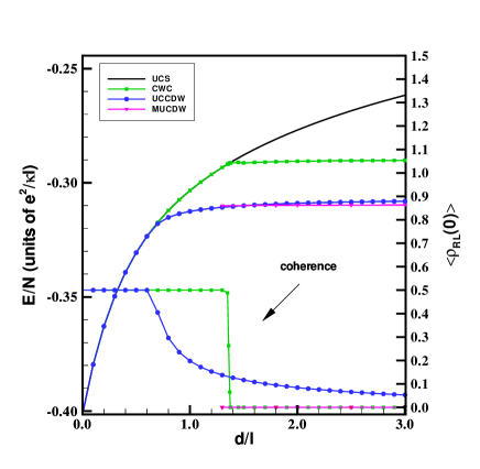
FIG. 1.: Hartree-Fock energy per electron and coherence as a function of the interlayer separation in the UCS, CWC, UCCDW and MUCDW states in Landau level $N=2$ and for $t=0$.

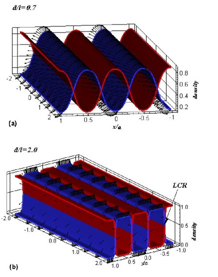
FIG. 2.: Real space representation of the guiding center and pseudospin densities in the UCCDW for $N=2$ and $t=0$. (a) $d/\ell=0.7$; (b) $d/\ell=2.0.$ The width of the linear coherent regions (LCR’s) become narrower as the interlayer separation increases.

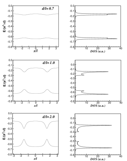
FIG. 3.: Evolution of the band structure $E\left(X\right)$ and of the density of states (DOS) in the UCCDW at $N=2$ and $t=0$ as a function of the interlayer separation. The interstripes separation is approximately $a=6.2\ell$ for these values of $d.$

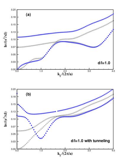
FIG. 4.: Dispersion relations calculated in the GRPA (a) without and (b) with tunneling for the lowest-energy collective excitations in the UCCDW in Landau level $N=2$ and for $d/\ell=1.0.$ These dispersions are for wavevector ${\bf k}$ in the direction of the stripes ($k_{\bot}=0$). The filled diamonds represent the phonon modes (in-phase and out-of-phase) while the lowest two branches of the $XY$ mode are represented by the empty squares.

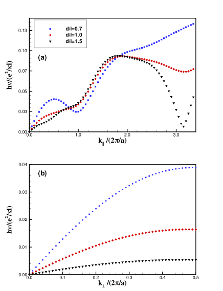
FIG. 5.: Dispersions of the $XY$ mode of the UCCCW with $N=2$ and $t=0$ for wavevector (a) parallel ($k_{\bot}=0$) and (b) perpendicular ($k_{\|}=0$) to the stripes and for several values of the interlayer separation.

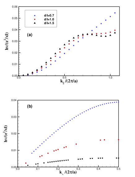
FIG. 6.: Dispersions of the in-phase phonon mode of the UCCCW with $N=2$ and $t=0$ for wavevector (a) parallel ($k_{\bot}=0$) and (b) perpendicular ($k_{\|}=0$) to the stripes and for several values of the interlayer separation.

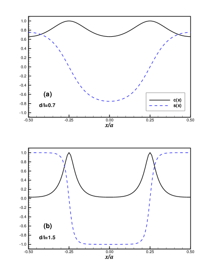
FIG. 7.: Plots of the functions $c(x)$ and $s(x)$ defined in Eq. (64) for the UCCDW in $N=2$ and for $t=0$. (a) $d/\ell=0.7$; (b) $d/\ell=1.5$.

REFERENCES

• [1] See, for example, S. Das Sarma and A. Pinczuk, eds., Perspectives in Quantum Hall Effects, (Wiley, New York, 1997).
• [2] M.P. Lilly, K.B. Cooper, J.P. Eisenstein, L.N. Pfeiffer and K.W. West, Phys. Rev. Lett. 82, 394 (1999); R.R. Du, D.C. Tsui, H.L. Stormer, L.N. Pfeiffer, K.W. Baldwin and K.W. West, Solid State Comm. 109, 389 (1999).
• [3] A.A. Koulakov, M.M. Fogler and B.I. Shklovskii, Phys. Rev. Lett. 76, 499 (1996).
• [4] R. Moessner and J.T. Chalker, Phys. Rev. B 54, 50006 (1996).
• [5] R. Côté and H.A. Fertig, Phys. Rev. B 62, 1993 (2000).
• [6] E. Fradkin and S.A. Kivelson, Phys.Rev.B 59, 8065 (1999).
• [7] H.A. Fertig, Phys. Rev. Lett. 82, 3693 (1999).
• [8] Hangmo Yi, H.A. Fertig, and R. Côté, Phys. Rev. Lett. 85, 4156 (2000).
• [9] D.G. Barci, E. Fradkin, S.A. Kivelson, V. Oganesyan, preprint, cond-mat/0105448 (unpublished).
• [10] The effect of quantum fluctuations on the spatial symmetry of the ground state is at present controversial. See A.H. MacDonald and M.P.A. Fisher, Phys. Rev. B 61, 5724 (2000); A. Lapatnikova, S. Simon, B.I. Halperin, and X.G. Wen, preprint, cond-mat/0105079 (unpublished). At any experimentally accessible temperature, the stripe crystal is surely destabilized (see Ref. [5]).
• [11] M.M. Fogler and V.M. Vinokur, Phys. Rev. Lett. 84, 5828 (2000); E. Fradkin, S.A. Kivelson, E. Manousakis, and K. Nho, Phys. Rev. Lett. 84, 1982 (2000); C. Wexler and A. Dorsey, Phys. Rev. B 64, 115312 (2001).
• [12] For a review, see article by S.M. Girvin and A.H. Macdonald in Ref. [1].
• [13] H.A. Fertig, Phys. Rev. B 40, 1087 (1989).
• [14] I. B. Spielman, J. P. Eisenstein, L. N. Pfeiffer, and K. W. West, Phys. Rev. Lett. 87, 036803 (2001).
• [15] X.G. Wen and A. Zee, Phys. Rev. Lett. 69, 1811 (1992).
• [16] Z. F. Ezawa and A. Iwazaki, Phys. Rev. B. 47, 7295 (1993).
• [17] I. B. Spielman, J. P. Eisenstein, L. N. Pfeiffer, and K. W. West, Phys. Rev. Lett. 84, 5808 (2000).
• [18] L. Brey and H.A. Fertig, Phys. Rev. B 62, 10268 (2000).
• [19] For $N=0$, the range of $d$ values for which the unidirectional modulated state is the Hartree-Fock groundstate is very narrow. See R.Côté, L.Brey and A.H.MacDonald, Phys.Rev.B 46, 10239 (1992).
• [20] E. Demler, C. Nayak, and S. Das Sarma, Phys. Rev. Lett. 86, 1853 (2001).
• [21] C.C. Li, J. Yoon, L.W. Engel, D. Shahar, D.C. Tsui, and M. Shayegan, Phys. Rev. B 61, 10905 (2000).
• [22] See article by A. Pinczuk in Ref. [1].
• [23] R. Côté and A.H. MacDonald, Phys. Rev. Lett. 65, 2662 (1990); Phys. Rev. B 44, 8759 (1991).
• [24] T. Nagamiya, in Solid State Physics 70 , F. Seitz, D. Turnbull, and H. Ehrenreich, eds., (Academic Press, New York, 1967).
• [25] C.S. O’Hern, T.C. Lubensky, and J. Toner, Phys. Rev. Lett. 83, 2745 (1999).
• [26] The use of long-wavelength commutation relations is only approximately valid for the states we are studying, which have a pseudospin density wave. However, the wavelength of this density wave is very large compared to the magnetic length [3], so that the additional factors in the microscopic operator commutation relations may still be set to their long-wavelength values without incurring significant error.
Refer to caption